Article

Determinants of Above-Ground Biomass and Its Spatial Variability in a Temperate Forest Managed for Timber Production

by
María De los Ángeles Soriano-Luna
1,
Gregorio Ángeles-Pérez
1,*,
Mario Guevara
2,
Richard Birdsey
3,
Yude Pan
4,
Humberto Vaquera-Huerta
1,
José René Valdez-Lazalde
1,
Kristofer D. Johnson
4 and
Rodrigo Vargas
2
1
Postgrado en Ciencias Forestales, Colegio de Postgraduados, Texcoco, Edo. de México 56230, Mexico
2
Department of Plant and Soil Sciences, University of Delaware, Newark, DE 19716, USA
3
Woods Hole Research Center, Falmouth, MA 02540-1644, USA
4
Northern Research Station, US Forest Service, Newtown Square, PA 19073, USA
*
Author to whom correspondence should be addressed.
Forests 2018, 9(8), 490; https://doi.org/10.3390/f9080490
Submission received: 13 July 2018 / Revised: 5 August 2018 / Accepted: 9 August 2018 / Published: 11 August 2018
(This article belongs to the Special Issue Forest Structural Dynamics in the 21st Century)

Abstract

:
The proper estimation of above-ground biomass (AGB) stocks of managed forests is a prerequisite to quantifying their role in climate change mitigation. The aim of this study was to analyze the spatial variability of AGB and its uncertainty between actively managed pine and unmanaged pine-oak reference forests in central Mexico. To investigate the determinants of AGB, we analyzed variables related to forest management, stand structure, topography, and climate. We developed linear (LM), generalized additive (GAM), and Random Forest (RF) empirical models to derive spatially explicit estimates and their uncertainty, and compared them. AGB was strongly influenced by forest management, as LiDAR-derived stand structure and stand age explained 80.9% to 89.8% of its spatial variability. The spatial heterogeneity of AGB varied positively with stand structural complexity and age in the managed forests. The type of predictive model had an impact on estimates of total AGB in our study site, which varied by as much as 19%. AGB densities varied from 0 to 492 ± 17 Mg ha−1 and the highest values were predicted by GAM. Uncertainty was not spatially homogeneously distributed and was higher with higher AGB values. Spatially explicit AGB estimates and their association with management and other variables in the study site can assist forest managers in planning thinning and harvesting schedules that would maximize carbon stocks on the landscape while continuing to provide timber and other ecosystem services. Our study represents an advancement toward the development of efficient strategies to spatially estimate AGB stocks and their uncertainty, as the GAM approach was used for the first time with improved results for such a purpose.

1. Introduction

Forests play an important role in mitigating climate change by fixing about 30% of fossil fuel CO2 (C) emissions [1,2,3]. Temperate forests constitute about 25% of the world forest area and store some 14% of the total forest carbon [1,4]. At a global scale, 44% of the world forests are under some sort of management regime [5], and forest management has been a very significant factor contributing to the current terrestrial carbon sink of 2.4 Pg C, accounting for about 0.7 Pg C annually [1,3]. Managed forests are critically important to assisting with reducing atmospheric CO2 concentration through initiatives like Reducing Emission from Deforestation and Forest Degradation, which includes the conservation and sustainable management of forests and enhancement of forest carbon stocks (REDD+) [6]. To implement the REDD+ scheme, assessing forest biomass stocks with a reliable accuracy is fundamental for project planning, and supports monitoring, reporting, and verification (MRV). Forest carbon stocks are usually calculated using AGB since typically 50% of AGB is carbon [7]. Incomplete information regarding the spatial variability (spatial distribution) of forest AGB introduces substantial uncertainty about current estimates of the carbon stocks present in managed forests and the global carbon budget [8,9]. Therefore, it is important to improve our knowledge of the spatial variability of forest biomass and its associated uncertainty in order to: (a) improve estimates of carbon stocks and understand carbon cycles [10]; (b) support future climate mitigation actions [11]; and (c) support sustainable forest management [12].
While timber production (usually evaluated as wood volume [13]) used to be the primary forest management’s objective (about 1.53 billion m3 per year in 2011) [14], some studies recognize the role of managed forests in contributing to carbon sequestration [15]. Forest management may enhance C sequestration in managed forest ecosystems [16,17] and optimize sink strength by using biofuels as substitutes for fossil fuels [3,18,19], while continuing to meet the timber demand of society [15]. There are mitigation opportunities involving forestry activities that could increase the gross terrestrial C uptake from roughly 4.0 to 6.2 Pg C annually [3]. This suggests the importance of assessing the AGB and timber production in managed forests to evaluate their contribution to climate change mitigation.
The AGB spatial variability and associated uncertainty, as well as the methods used to minimize it, have attracted considerable attention [20]. An uncertainty map at the pixel level is valuable for the interpretation of the AGB map [21,22] and for reporting emissions. The development of remote sensing technology combined with intensive site-based inventory approaches for estimating forest biomass stocks and forest area changes, are important for addressing monitoring problems and implementing REDD+ [23]. The combination of remote sensing and field measurements contributes to a robust and transparent MRV system.
The carbon pools in managed forests are affected by different drivers, mostly by forest management regimes and natural disturbances [24,25,26,27], the species composition of forests and forest type [28,29], plus the age structure [30,31]. AGB and carbon in forest ecosystems are also strongly affected by climate [24,32,33], as well as soil properties and topography [34,35,36]. However, it is difficult to clearly attribute the effect to forest management or other environmental factors [3]. Therefore, understanding the factors determining AGB spatial variability at the landscape level is a first step for properly estimating AGB through a prediction method.
The prediction method has a substantial effect on the accuracy of AGB estimates. Linear models are among the most popular choices for estimating AGB because of their simplicity and interpretability when compared to other models, such as random forest methods and Gaussian processes [37]. Random forest methods have performed well in many cases, while stepwise linear models are often the least effective, judging by r2 and RMSE with cross-validation [38]. Other model approaches such as the generalized additive models (GAMs) may describe a complex relationship between the response variable and its predictors. This is especially useful in research fields such as ecology or biology in which simple models cannot capture the structure of the data and more complex models may be required [39]. However, this approach has not been used to assess the spatial variability of AGB. In addition, LiDAR technology has proven to be a valuable tool in mapping the spatial variability of AGB [21]. This type of high-resolution data offers great improvement for AGB estimation and can reduce its uncertainty in accordance with the Intergovernmental Panel on Climate Change (IPCC)’s Tier 3 for the forestry sector [20,38].
In this study, we used three types of models to characterize the spatial variability of AGB in managed forests in central Mexico. Mexico is covered by 65 million hectares of forests [5,40] with a variety of forest ecosystems (i.e., 51% temperate forests, 49% tropical forests) [41] due to its geographical location and topographic heterogeneity. Forests in Mexico are important for their current and potentially increasing accumulation of C in their biomass [42,43,44]. However, there is a lack of information on the spatial variability of AGB and the determinants that affect it, especially in managed forests (11% of total forested area within Mexico) [40,41]. Therefore, the objectives of this study were: (1) to analyze the determinants of AGB and its spatial variability in a managed forest landscape for timber production; (2) to evaluate the effect of different models (using the same input variables) for predicting AGB; and (3) to estimate the AGB estimation uncertainty across the forest landscape. We expected that AGB is driven by stand structure, climate, and topography; and that the prediction method has a substantial effect on the AGB estimates and uncertainty. This work is novel as it is the first known study that uses a GAM model to map AGB, which is compared to other commonly used models.

2. Materials and Methods
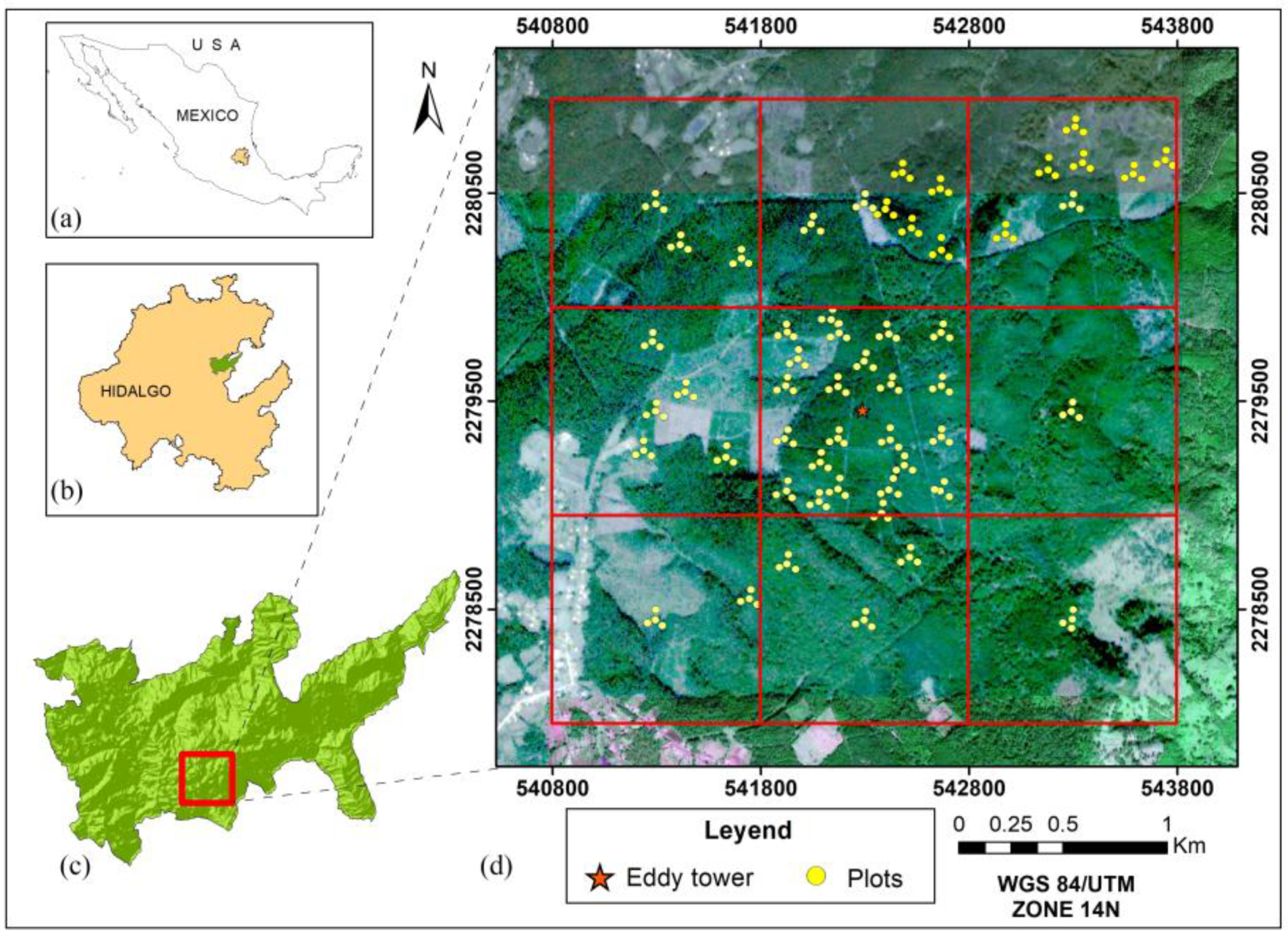
2.1. Study Site

We conducted the present study in a Mexican temperate forest in the Zacualtipán forested region, in the state of Hidalgo (20°37′4978′′ N and 98°37′51.01′′ W and 20°35′18.74′′ N and 98°35′23′′ W), central Mexico (Figure 1). This site is a member of the Mexican Network of Intensive Carbon Monitoring Sites (MEX-SMIC, its acronym in Spanish) [45,46], and the MexFlux network [47]. From the 1980′s, communities that own these forests started Forest Management Programs for timber production, generating even-aged stands of Pinus patula Schltdl. et Cham. through the seed-tree regeneration method. Natural regeneration is also combined with artificial reforestation (enrichment planting) when natural regeneration is insufficient. Thinning is the most common silvicultural treatment applied for producing wood for commercial purposes, decreasing competition between the remaining trees, and controlling tree species composition. Mountain cloud and pine-oak forest that is 80 years old, with no silviculture activities applied (designated as reference forest), represents 31% of the study area. The predominant climate is humid with summer rains averaging 2050 mm and an average annual temperature of 13.5 °C [48], both varying according to elevation and aspect. The typical phaeozem haplic soils (Hh) are rich in organic matter, and in the areas with steep slopes, calcaric regosol (Rc) soils are found [49].

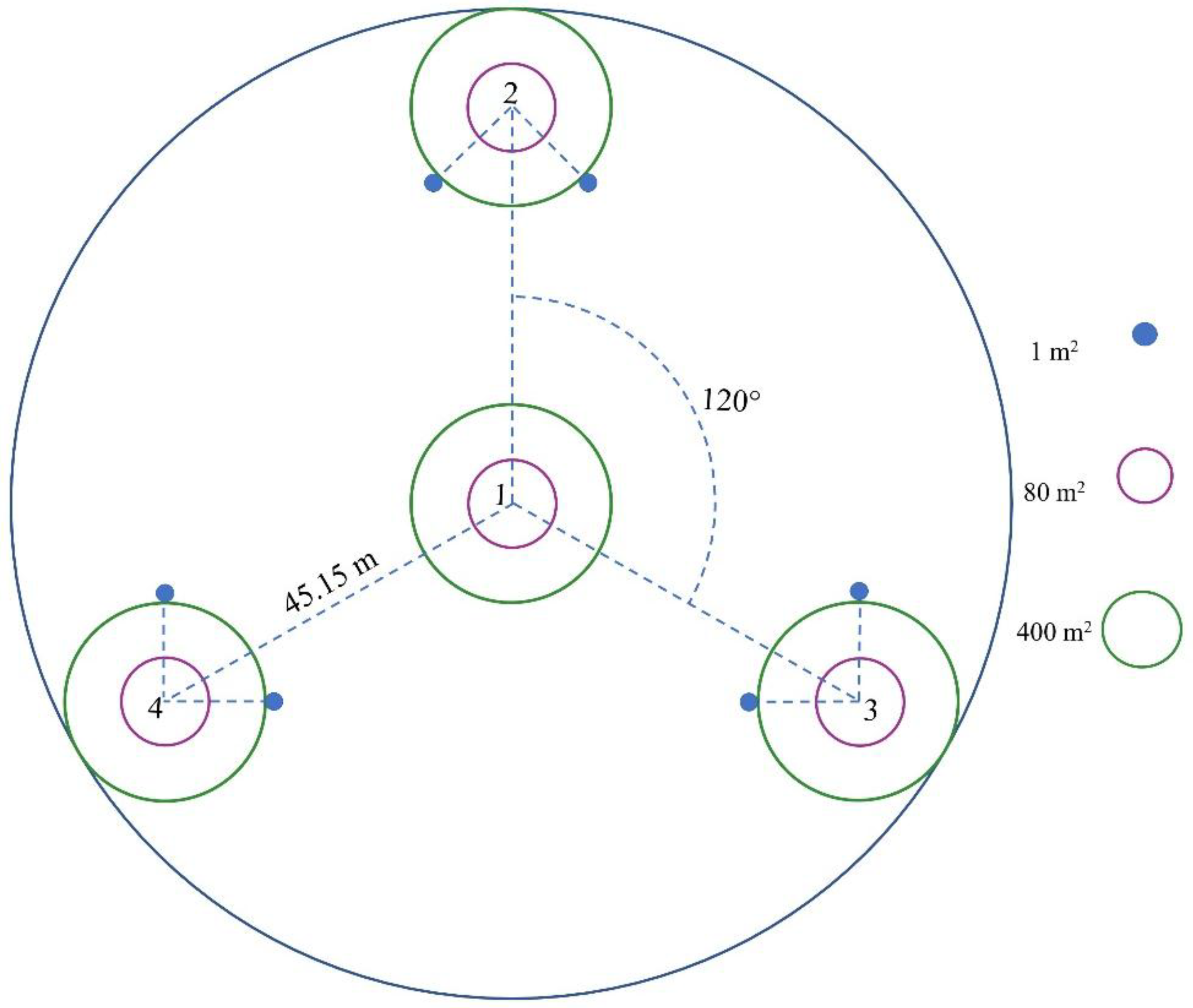
2.2. Permanent Sampling Plots

The intensive carbon monitoring site was established during 2012–2013 across a 3 × 3 km land area, adapting guidelines developed for similar monitoring sites in the U.S. [50]. A flux tower was instrumented in the center of the polygon in order to provide direct estimates of energy, carbon dioxide, and water fluxes. We established 24 permanent inventory plots following a systematic pattern and 27 plots randomly located following a gradient of harvesting years to spatially sample a forest recovery chronosequence, including a reference forest. The additional plots enabled a more effective representation of the variability of ecosystem carbon stocks (live biomass, dead organic matter, and soils) across the managed forest landscape. Sampling protocols were consistent with the design of the Mexican national forest inventory (Inventario Nacional Forestal y de Suelos—INFyS) [51], but included many more variables generally following the standard protocols described in Hoover [52]. We delimited 11.28 m radius subplots (400 m2 area) to measure trees with a diameter at breast height (DBH) of ≥5 cm. Additionally, 5.04 m radius microplots (80 m2) were employed to measure trees with 2.5 ≤ DBH < 5 cm and taller than 1.3 m. Understory biomass (herbs, shrubs, and trees < 2.5 cm in diameter) was destructively sampled at two circular microplots of 1 m2 per subplot (two on each of the secondary sampling units 2, 3, and 4) (Figure 2).

2.3. Field Measurement and AGB Estimates

Field data consisted of individual tree information recorded during 2013. We used 204 subplots of 400 m2, 204 microplots of 80 m2, and 240 microplots of 1 m2 in order to quantify the AGB defined as all living vegetation, both woody and herbaceous, above the soil [20]. All plots were geo-referenced on the ground with a GPS Garmin GPSmap® 62 s [53]. We tagged all trees, identified species, and measured the DBH at a 1.3 m height of live trees ≥ 5 cm diameter in the 400 m2 plots, and trees with 5 > DBH > 2.5 cm and taller than 1.3 m in the 80 m2 subplots. When irregularities (e.g., bole irregularities, buttress roots) were present at the sampling height, we took DBH measurements 5 cm above the irregularity [54]. We also recorded the total height of each tree. The total number of plots amounted to 204, where we examined and measured 11,015 trees.
We measured understory biomass (herbs, shrubs, and trees < 2.5 cm) in 240 microplots of 1 m2 by destructive sampling, took sub-samples to the laboratory, and oven-dried them at 70° for dry weight determination. The chronosequence in managed forest covered 31 years. More than 31 units (stands) of different ages were identified from one to 31 years old. The stand age was defined as the time since harvesting. It was obtained during the field survey and from forest management plans. GIS-based forest inventory polygons were used to extract the age for each stand in the complete area. The reference forest showed no recent harvesting or disturbance, and has an estimated age of 80 years [55]. We used four to 20 plots per stand age according to the stand area (Figure 1), except for the 31-year stand, where only one plot was used. We estimated AGB (oven dry mass) by applying local species-specific allometric equations [55] (Table 1). For each plot, we computed the AGB per plot by summing all sample tree biomass estimates. Next, we obtained the biomass values in megagrams per hectare (Mg ha−1) considering the size that each plot or subplot represented (0.04 and 0.008 ha). We estimated understory biomass per 1 m2 microplot by using the ratio dry weight:total fresh weight and extrapolated to biomass per hectare (ha). Additionally, for each plot, we computed the basal area per hectare (m2 ha−1) and tree density (N ha−1).

2.4. LiDAR Data

We acquired LiDAR returns and feature heights in ASPRS LAS file format (American Society for Photogrammetry and Remote Sensing, LASer file format) and the Digital Terrain Model, as LiDAR-derived bare earth elevation (m, EGM96 geoid) in raster data (GeoTIFF) at a nominal 1 m spatial resolution, through the Goddard’s Lidar, Hyperspectral, & Thermal imager (G-LiHT) webpage [57]. LiDAR data was collected in April 2013 in an attempt to avoid clouds associated with the rainy season [58]. We processed LiDAR data using FUSION software version 3.60+ [59]. We calculated LiDAR metrics [59] (Table 2), the mean, and the standard deviation values from the cloud of points within all the study sites in the 3 × 3 km landscape at a 5 m resolution. We used a threshold of 2 m as a minimum height above ground to reduce the noise within the near-ground cloud of returns caused by low vegetation and imperfections of the ground. A canopy threshold height (height break above the ground) of 3.0 m was used to compute LiDAR canopy cover metrics according to the specific characteristics of the study site [53]. We used the LiDAR metrics as predictor variables in the models for estimating the spatial variability of AGB.

2.5. Climatic and Topographic Data

Since the sampled plots did not have climate data at a fine spatial resolution, we gathered meteorological data from recording stations in the region. First, we resampled the 1 m DTM into a 5 × 5 m pixel size grid by using the downscaling method of bicubic spline [60] implemented in the System for Automated Geoscientific Analysis (SAGA) software v2.2 [61]. Then, we used R programming language [62] to fit annual mean temperature (AT) and annual total precipitation (AP) models by using a LiDAR-derived digital terrain model (DTM). Temperature was strongly correlated with latitude and elevation, while precipitation was better correlated with latitude and longitude. We estimated the AT and AP by applying the fit equations at the pixel level (using latitude, longitude, and elevation) for the entire study area.
We obtained topography parameters by using the LiDAR-derived DTM (1 m resolution) [57,61]. SAGA software was used for the analysis of spatial data, and to derive the primary topographic metrics [63]: Analytical Hillshading, Slope, Aspect, Plan Curvature, Profile Curvature, Convergence Index, Closed Depressions, Total Catchment Area, Topographic Wetness Index, LS-Factor, Channel Network Base Level, Channel Network Distance, Valley Depth, and Relative Slope Position, according to Wilson [64] (Table 2).

2.6. Statistical Models and Analysis

All data were harmonized in a geographic information system and we applied a clipping process from the gridded information (stand age, LiDAR metrics, climatic and topographic parameters) at the 198 plots (400 m2) with SAGA [61].
We developed several kinds of models to fit our data for predicting the AGB density (Mg ha−1) across the landscape (spatial variability of AGB) from the set of predictor variables (Table 2): empirical statistical models, a multiple linear model (LM), generalized additive models (GAM) [65], and Random Forest (RF) [66] using 10–fold repeated cross-validation [67]. All the analyses were conducted in the R programming language [62]. We analyzed all possible combinations between variables to understand which predictors had more weight in the explanation of the spatial variability of AGB and thereby to interpret the main significant effects.
We used LM to identify highly-correlated variables and determine the best-fit. In order to find a model with the greatest explanatory power, a backward stepwise multiple linear regression was performed to automate the selection of the best explanatory variables. Multiple regressions are often affected by overfitting and co-linearity among variables. Multicollinearity was tested by the variance inflation factor (VIF) [68]. We removed the variables with a VIF above 5 from the model. Bootstrap samples were used from the data to implement the 10–fold cross-validation analysis.
We fitted GAM, a semi-parametric approach [65], for predicting the nonlinear responses of biomass to the set of predictor variables. GAMs are regression models that generalize the family of generalized linear models (GLMs), by replacing the linear functional form with a sum of smooth functions [69,70]. GAMs have been strongly accepted in several domains as a flexible modeling technique, suited for capturing nonlinear, unspecified relationships between predictor variables and the response variable [71,72]. GAM has been used to explore the AGB [73], but not to map its spatial variability. In this study, we performed GAM regression assuming a Gaussian error distribution. GAM regression was carried out using the R packages mgcv [74], and gamclass [75] to implement the 10–fold cross-validation. Stepwise selection using the Akaike information criterion (AIC) [76] was used to control the complexity of the GAM model.
The RF algorithm [66] was used as the other prediction model. RF is a machine learning algorithm that has been proven to reduce bias and overfitting. It works well with random inputs, and in some cases, tends to be more accurate than simple regression techniques for biomass estimation [37]. We used the rfcv function within the randomForest package [77] for the 10-fold cross validation analyses. The search of the covariates was pursued with the tune.randomForest function in the R e1071 [78] and VSURF [79] packages, with 1000 iterations of bootstrapping to improve performance estimates and control over-fitting.
For accuracy assessment, we used the 10–fold repeated cross-validation [67] (each model was re-fitted 10 times using 90% of the data and predictions derived from the fitted models were compared with observations of the remaining 10%) [80]. We derived the coefficient of determination (R2) and root mean squared error (RMSE) to quantify the goodness of fit of the models. Those with the lowest AIC [76] root mean square error (RMSE) and the highest R2 (adjusted for number of predictors in the model) were considered [81]. Finally, we applied spatial prediction models using tiled raster stacks (covariates) to map the AGB by using the R raster package [82].

2.7. Uncertainty Quantification

To estimate the potential uncertainty of AGB predictions, we used the difference of 95% prediction intervals (0.925–0.025) to calculate the absolute values of AGB uncertainty (Mg ha−1) per pixel by LM and GAM methods. For a normal distribution, this interval would be about ± 2 standard deviations about the mean. This uncertainty is limited to prediction error and serves as a reference to which the uncertainty due to model selection can be compared. This uncertainty represents the amount of AGB that cannot be explained for the predictor variables.
To estimate the uncertainty of the RF AGB predictions, we used the Quantile Regression Forests (QRF) approach to infer a pixel-based full conditional distribution [83] of the AGB response to predictors given available data. The statistical distribution of predicted values per pixel, estimated as the 95% prediction intervals, was obtained using the quantreg Forest package in R [84]. This technique allows a non-parametric and alternative way of estimating the reliability of AGB predictions.

3. Results

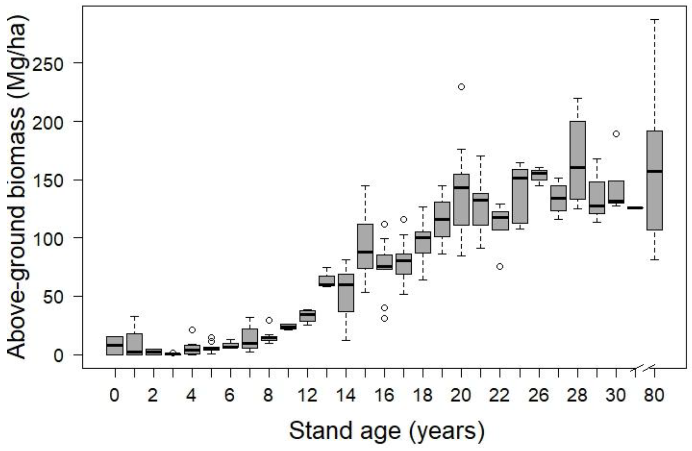
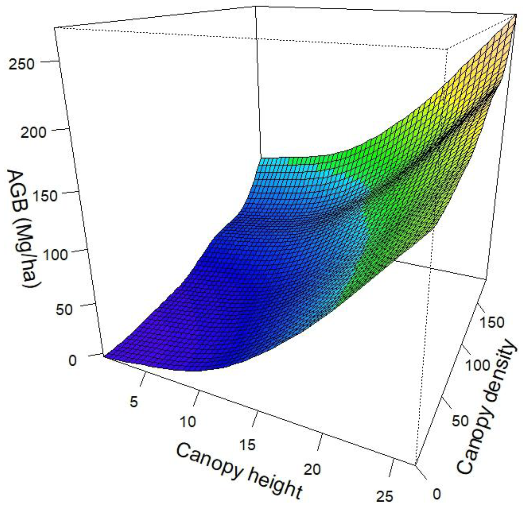
3.1. AGB and Effects of Forest Structure

AGB of trees >5cm varied from 0.49 ± 0.66 to 166.6 ± 42.4 Mg ha−1 in stands ranging from three to 28 years old (Figure 3). Some recently harvested stands have up to 30 Mg ha−1 because of the seed trees remaining which are removed after regeneration is established. Biomass in trees of diameter class 2.5–5cm DBH ranged from 0 to 4.6 ± 1.3 Mg ha−1, increasing with stand age, but not significantly. Understory biomass varied from 1.1 ± 0.7 to 12.8 ± 7.4 Mg ha−1, but did not show a trend with increasing stand age. The reference forest had an average AGB of 159.5 ± 67.4 Mg ha−1, which was not statistically different (p > 0.05) from managed older stands (20–28 years). However, it is noteworthy that the old-growth stand reached a maximum AGB of 287.3 compared to 223.4 Mg ha−1 in some managed older stands (Figure 3). Tree density and basal area were positively correlated with the AGB (p < 0.0001). They explained up to 90% of its variability. However, these forest management variables are not usually mapped.
LiDAR-derived forest metrics were strongly correlated with AGB. A canopy height metric (the 95th percentile height for all returns above 2 m) (eP95), and a canopy density metric (All returns above 3 m/first returns) × 100) (a1a3), were the two most significant predictors of AGB (p < 0.0001). Both forest structure variables showed positive effects in all the models (p < 0.0001) (Figure 4).

3.2. Climate and Topographic Variables

There were spatial patterns in the distribution of climatic values: precipitation increased from the southwest to the northeast, while temperature showed the opposite pattern. These variables did not individually influence the AGB, but the interaction between stand age and precipitation had a positive effect (p < 0.0001). Topographic factors, which mostly influenced temperature and precipitation patterns, had a limited effect on AGB. Slope and relative slope position as determined by LiDAR-derived DTM had a negative effect, while valley depth had a positive effect, on AGB (VIF < 1.2), explaining up to 11.4% of AGB variability (p < 0.0001).

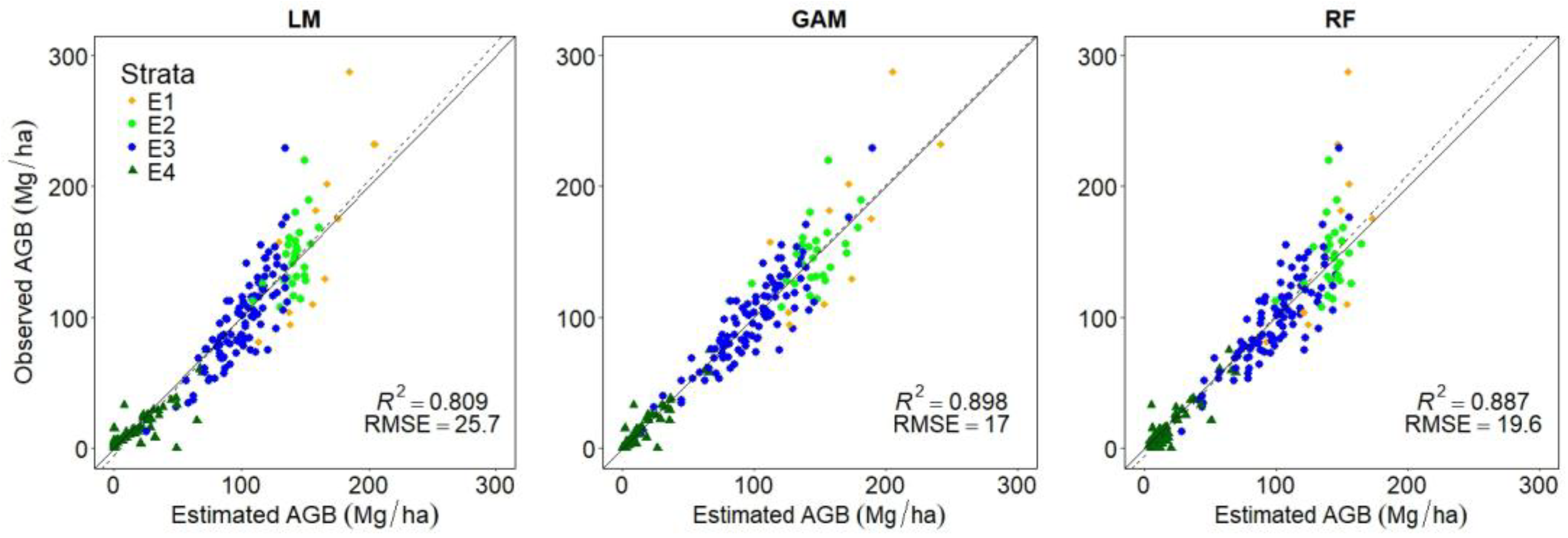
3.3. Spatial Prediction Models

The linear model explained 80.9% (AIC = 1782, RMSE = 25.7) of the spatial variability of AGB (Table 3). LIDAR-derived variables related to forest structure, which are the 95th percentile height for all the returns above 2 m (eP95), canopy density (all the returns above 3 m/first returns) × 100) (a1a3), and stand age (management variable), were the three most significant predictors of AGB (p < 0.0001). The optimal GAM model explained 89.8% (AIC = 1712, RMSE = 17) of the variability in AGB, having forest structure variables (height, density, and age) as the most significant predictors. This semiparametric approach confirmed the importance of forest management variables (eP95, a1a3, and stand age) (Table 3) because the management actions directly define them. The RF model also consistently showed forest management variables as the most important, explaining 88.7% (RMSE 19.6) of the AGB spatial variability.

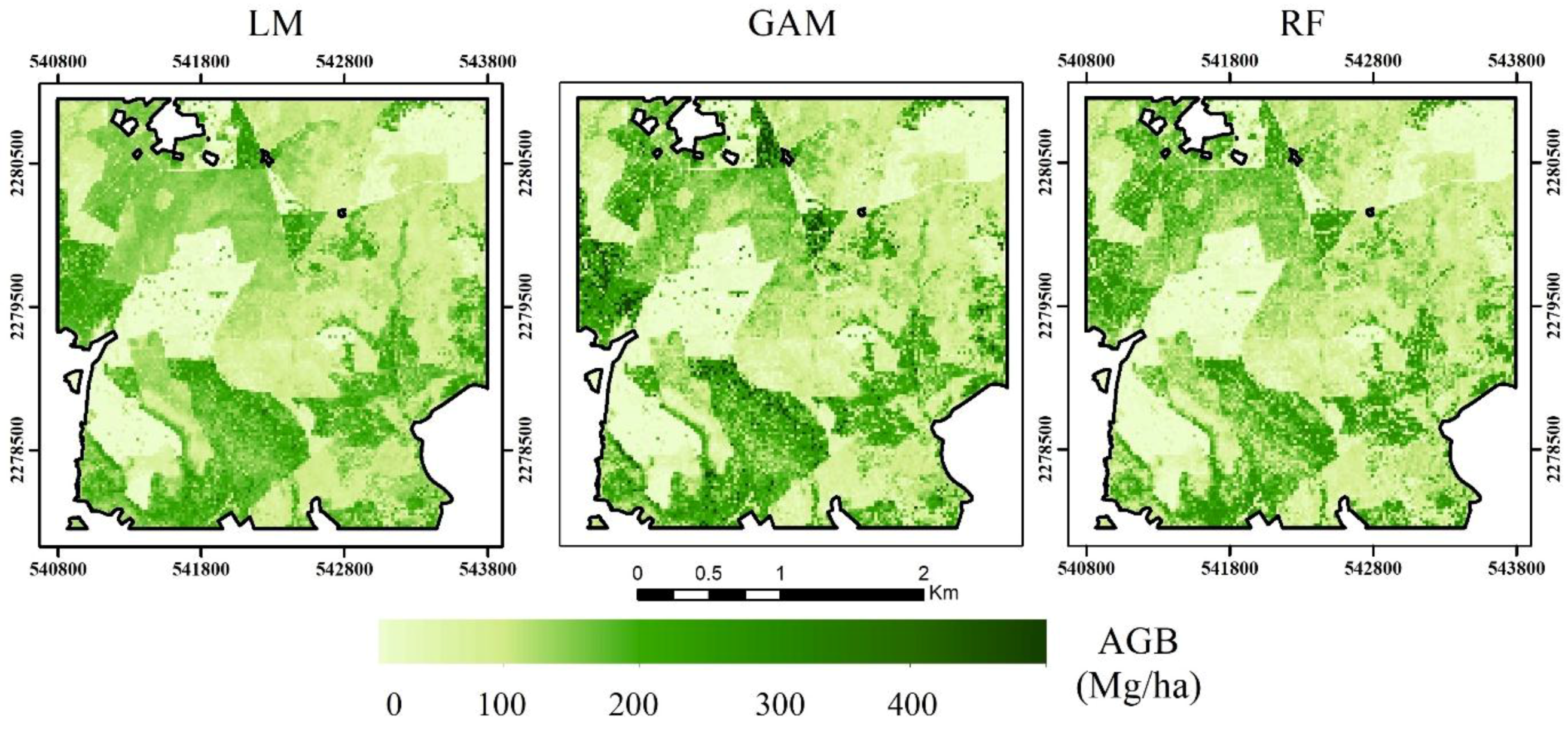
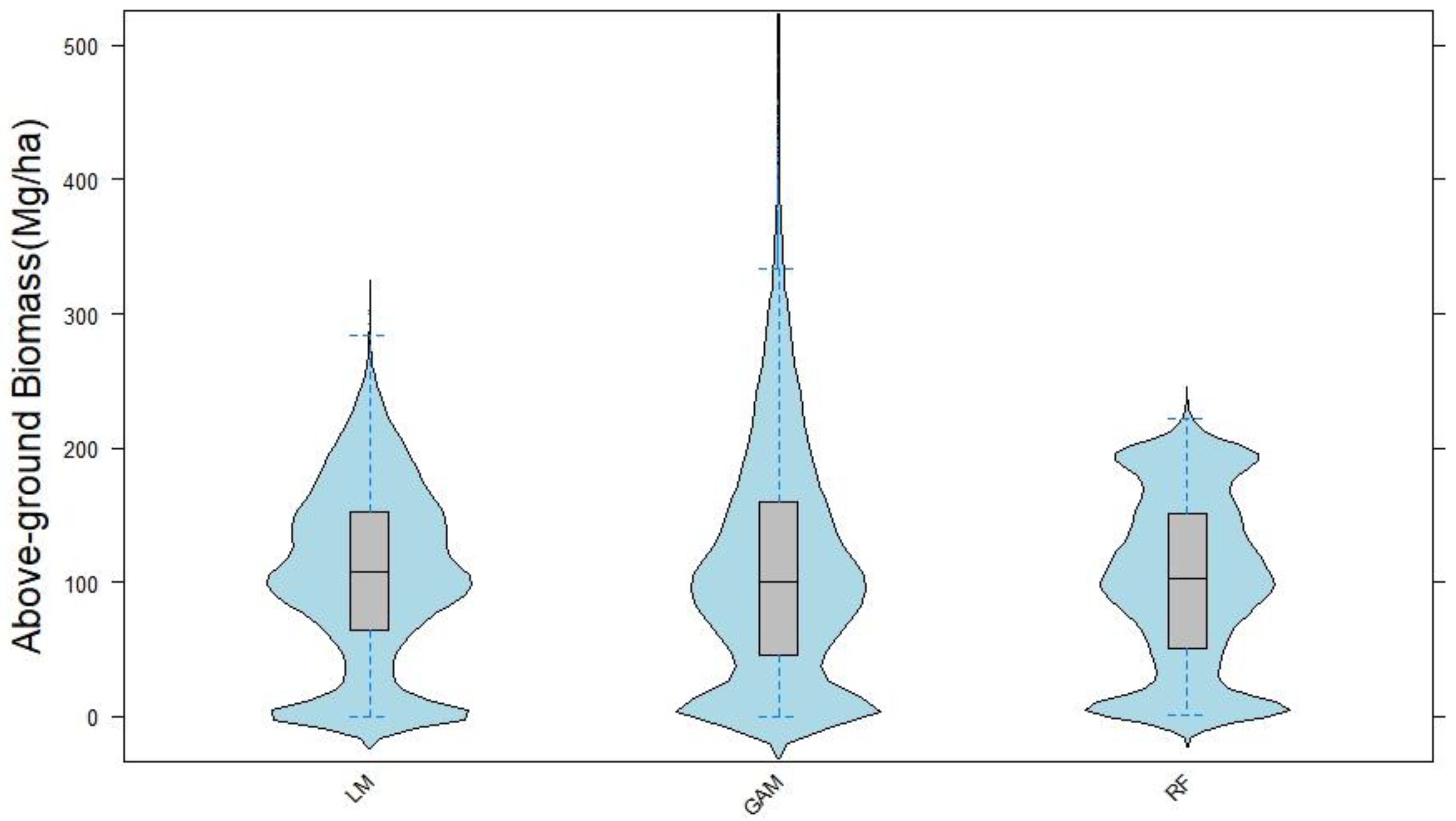
3.4. Spatial Variability of AGB

AGB varied across the forested landscape, driven mainly by forest structure and stand age (Figure 5). The three models overestimated AGB in the plots where measured biomass was very low or near zero, but they tended to underestimate AGB for plots with very high biomass measurements (Figure 6). LiDAR metrics performed well in predicting AGB variability. The prediction methods have an impact on AGB estimates. GAM predicted the highest values of AGB, while RF predicted more conservative values (Figure 7), with a 19% difference between methods.

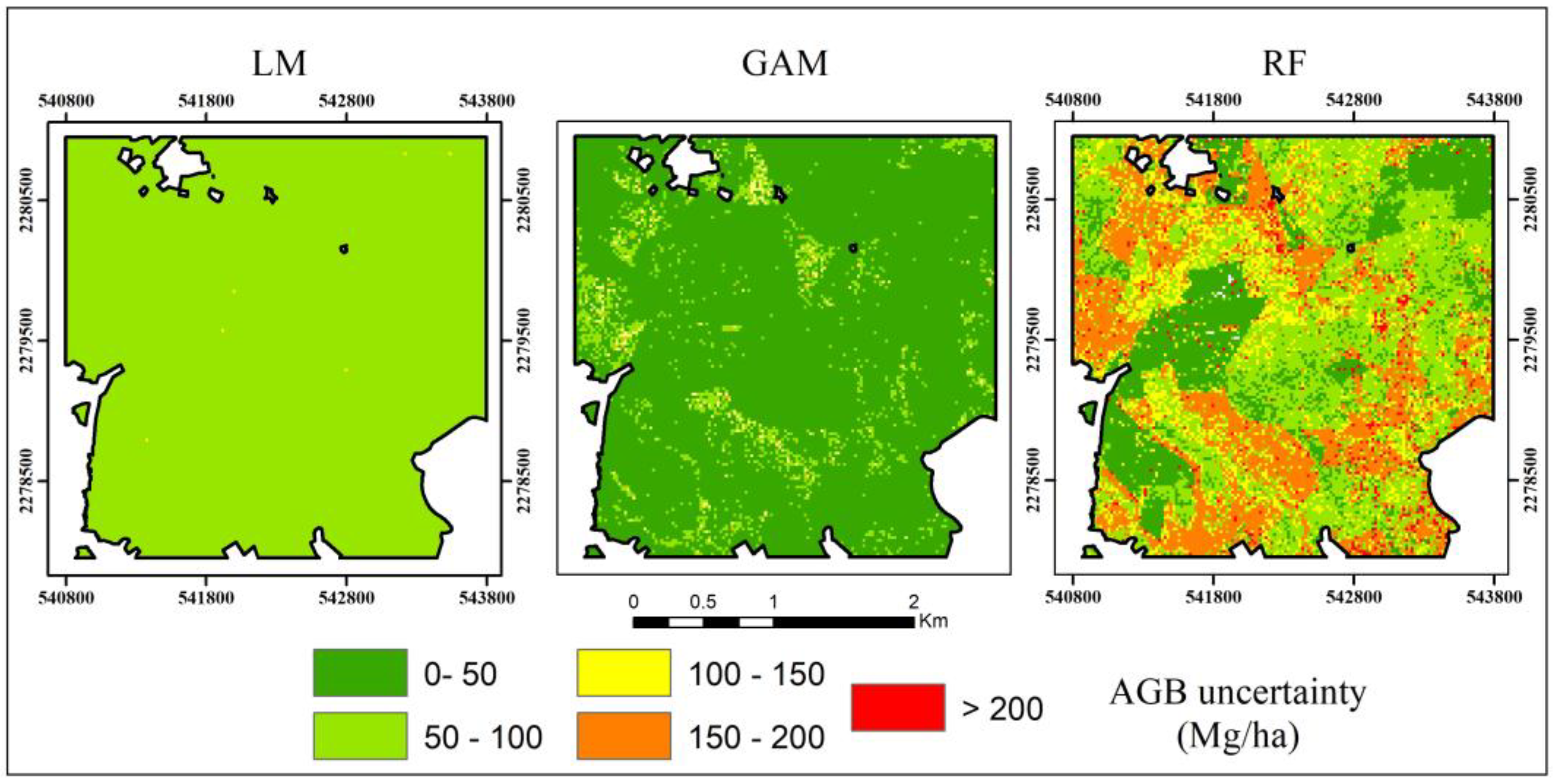
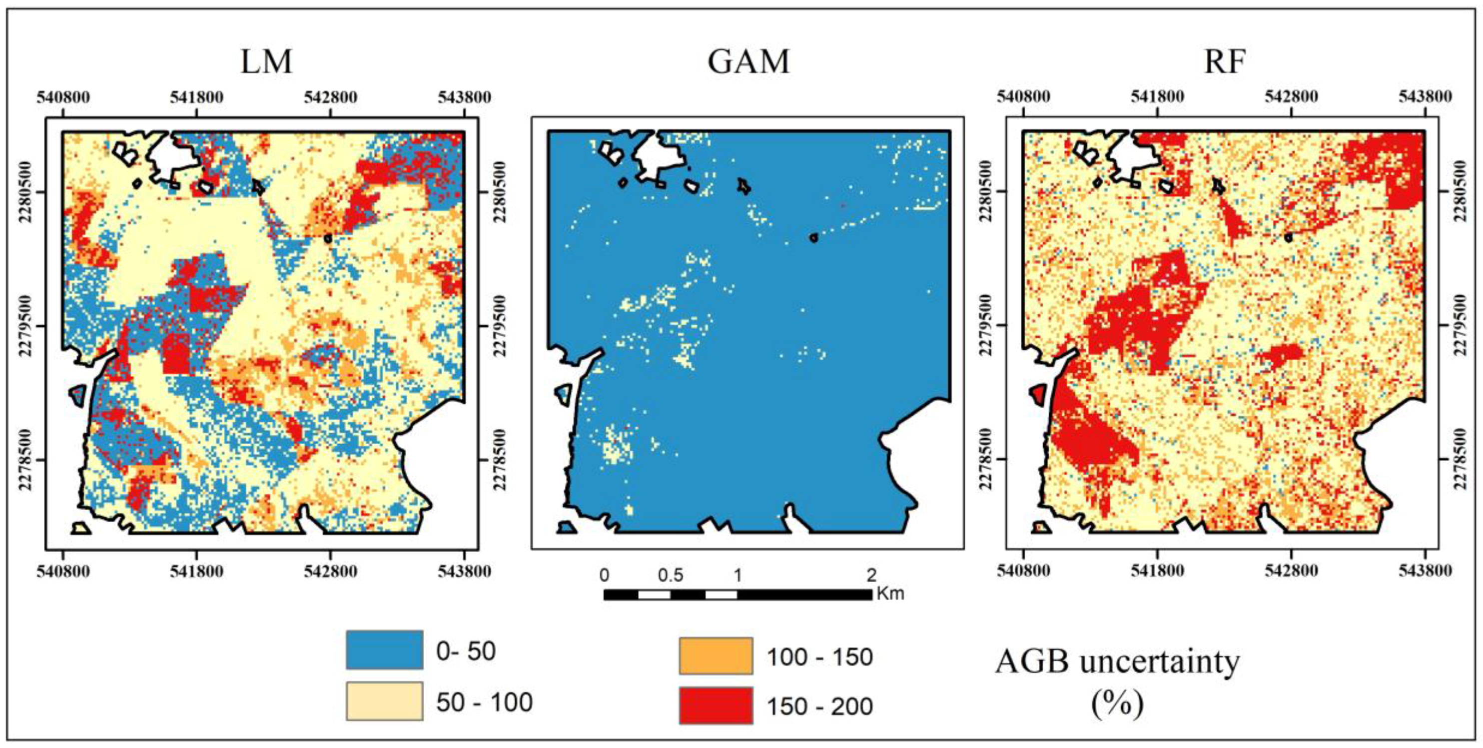
3.5. Mapping AGB Uncertainty

The highest uncertainty predicted (expressed by absolute values of AGB) by each prediction method was observed in areas associated with high AGB values (Figure 8). The uncertainty of the estimates, expressed as the range of the 95% confidence intervals divided by their mean (in standardized form) [85], was larger in young stands and open areas (Figure 9). The prediction method affected the AGB uncertainties, with the GAM method produced the lowest uncertainty values.

4. Discussion

We identified determinants of AGB and derived spatially explicit estimates by three empirical methods in a managed forest for timber production. AGB stocks were compared with an 80-year-old reference forest. Our results highlight the importance of including historic anthropogenic disturbances (i.e., forest management) for a better estimation of landscape-scale carbon dynamics and ultimately, the Mexican carbon budget as affected by climate mitigation activities. We emphasized the estimation of the AGB uncertainty by building a map that provides a detailed spatially explicit characterization of AGB uncertainty, which is a novel approach for better characterizing its variation across the landscape, identifying the most uncertain areas, and developing strategies to reduce it.

4.1. Spatial Variability of AGB

Plot-level AGB. Our plot-level AGB estimates across the chronosequence demonstrated how tree biomass increases with stand age. This pattern corroborates previous studies conducted in temperate forests [86,87], confirming that stand age is an important variable for estimating biomass in managed forests for timber production. Estimated AGB in our site was similar to other managed forests in the region [48,88,89], and higher than in some other pine-oak managed forests in México [90]. There was no statistical difference in AGB (>0.05) between the oldest managed stands (20–31-years-old) and the reference forest (Figure 3), revealing that forests managed for timber production in Mexico have a high potential to accumulate biomass and achieve high carbon stocks in a relatively short period of time. However, it is still necessary to integrate other carbon pools (i.e., below-ground biomass, soil organic carbon, etc.) into the analysis of managed forest carbon dynamics to fully quantify the impacts of management.
We noticed that AGB varied among stands of the same age, with smaller variation in young stands (sd = 2.2 Mg ha−1) but greater variation in old stands (sd = 42 Mg ha−1), and the greatest variation in the reference forest (sd = 64 Mg ha−1). Basal area and tree density controlled by management practices [15] such as thinning in our site [88] affected the AGB (p < 0.0001). Age-related differences in AGB among plots are also likely due to heterogeneous site conditions and species composition through variations in wood specific gravity [91], soils, microclimate, and human disturbances over time of forest development. The average AGB in the reference forests in our site was low compared with the range of temperate forests in North America (106–366 Mg ha–1) [4], although we did observe AGB > 280 Mg ha–1 in some plots (Figure 3). Most of the mature forests in our site are mixed pine-oak with a relatively low tree density. They appear to be nearing the old-growth stage with large gaps and more dead trees, which typically results in a lower average and a wide range of AGB (Figure 3). This suggests an opportunity to assess the role that biodiversity plays in determining AGB. Additionally, unmanaged natural forests have experienced natural disturbances, such as fire and storms affecting the AGB.

4.2. Estimation of AGB across the Landscape

Our results support using LiDAR-based estimates of biomass to improve AGB mapping and support management decisions. LiDAR information is well-suited for inferring forest height, as well as vertical and horizontal forest structure [37] such as canopy cover [92], which successfully estimated AGB across the landscape. Our findings support previous studies that show that AGB can be estimated using LiDAR and ground measurements with a higher accuracy than traditional assessments based on RMSE [93,94,95]. We found that the LiDAR-based AGB varied from values near 0 (recently harvested stand) to the highest values of 302 ± 25.7 and 492 ± 17 Mg ha−1 on the temperate forest landscape due to changes in forest structure and stand age, mainly attributed to forest management practices, that produced a mosaic of different age classes, tree heights and densities, and thus biomasses (Figure 3 and Figure 4). These AGB estimates were higher than the observed data from field sampling alone, suggesting the need to increase the sampling effort to capture a larger variability of forest structure and thus AGB. For forest and land managers, to have this detailed knowledge of the spatial distribution of AGB is helpful for designing silvicultural practices and harvesting schedules to increase carbon sequestration on their lands, in light of REDD+ and carbon mitigation programs.

4.3. Effects of Climate and Topography

Topography affects the AGB variability in forest landscapes [9,96]; however, in the present study, this influence was overshadowed by the various structural conditions existing in the stands that make up the forest, a product of the intensive management activities (silvicultural regime) implemented in the last 40 years. Slope and relative slope position had a negative effect on AGB. Valley depth was positively correlated with AGB, representing the vegetation remaining along rivers or streams to protect the water. While topography and climate explained 57% of the AGB in the reference forest, they only explained 11.4% of it in the managed forest, likely due to the conditions within stands derived from the planned silvicultural activities. However, this study provides critical information on disturbances, climatic, and topography which can be used to test and parameterize process-based models in temperate managed forest for assessing spatially explicit carbon dynamics.

4.4. Comparing Prediction Methods

The three AGB fitted models performed well when predicting AGB and associated spatial distributions (Figure 5, Figure 6 and Figure 7). Comparatively, GAM was better for representing ABG variations across the landscape (Figure 5 and Figure 7). These model results compare favorably to studies that reported larger RMSE values for biomass in California, USA (30–70 Mg ha−1) [97]; Yucatan, Mexico (37.4 Mg ha−1) [98]; and Germany (23–60 Mg ha−1) [99,100].
All fitted AGB models tended to overestimate AGB in sites with lower field values, and underestimate AGB in sites where measured AGB is high (Figure 6). This pattern is similar to previously reported studies [21,94,100], perhaps due to increasing forest structure differentiation with forest development, in contrast with the models representing more average conditions. Compared to LM, the RF method resulted in a better model performance, similar to previous studies [37,101]. However, in our case, the GAM method performed better than LM and RF based on RSME and R2. This method was previously applied with success in ecological and vegetation modeling [102,103]. Although the GAM method has only been used as an exploratory tool in biomass studies [8], in our study, the GAM method improved AGB predictions more than the other two methods. It showed high potential for use in similar analyses. GAMs may describe a complex relationship between the response and predictor variables. The resulting model suggests that AGB is primarily a function of stand age across the region. Therefore, generating a spatially-explicit age map is a necessary step for AGB estimation across larger regions where LiDAR data is not available.

4.5. Spatial Uncertainty

Several recent studies have incorporated more thorough statistical techniques to estimate the uncertainty of various biomass estimators across landscapes [104]; however, few studies have reported uncertainties in the spatial variability of AGB. In this study, we mapped the estimated uncertainty of AGB and identified the areas with high absolute values (Figure 8), which could assist land managers in better planning sampling strategies and management practices. Higher absolute values of uncertainty are associated with higher predicted values, showing that forest complexity may affect biomass predictions. A similar pattern was found by Su, et al. [21] in different forest types in China. The uncertainties of the estimates, expressed as the standardized range of the 95% confidence intervals (Figure 9), were generally small when observations were dense, and the highest in young stands and open areas, probably associated with the lack of mapping understory and small tree size (<5 cm DBH) biomass, which contributed up to 4.6 and 15.9 Mg ha−1, respectively. The variability in AGB due to remaining seed trees left after harvesting also could contribute to these uncertainties.
Additionally, we assumed the stand age based on the years after harvesting; however, the first successional stage of managed forest could last for several years, and forest structure variables related to age (i.e., basal area) may not represent the real stand age since some large scattered trees are left after harvesting due to the used regeneration method. Although useful, the lack of continuous spatial coverage of the predictors themselves (i.e., stand age) is a problem when one is attempting to use interpolation methods to spatially predict AGB. Therefore, it makes sense to use forest structure variables to better predict stand age in managed forest across larger areas in order to reduce AGB uncertainties.
This estimated uncertainty can result in different correlations between field-measured AGB and predictors. This suggests an opportunity to increase efforts to quantify the uncertainties associated with different sources of error that interact and propagate, such as measurement error, sampling error, the AGB allometric equation [105,106], plot location uncertainty, and the edge effect [21], to improve the estimates of AGB and carbon stocks. It is necessary to quantify the map uncertainty at different spatial scales including different sources of error. Nonetheless, the current study represents an important approach to reporting uncertainty for improving estimates of carbon stocks to support sustainable forest management, as envisioned by REDD + programs.

4.6. Improving AGB Estimates in Managed Forests

The implications of our study for estimating biomass carbon stocks and improving forest management are significant. Over the forested study site (∼823 ha), the AGB estimated by the LM method was 78,928.0 (±242) Mg, by the RF method was 86,356 (±220) Mg, and the GAM method was 94,654.0 (±190) Mg. These results are higher than those obtained by Torres-Vivar, et al. [89] using different approaches. In that study, the authors estimated 80,431 Mg of AGB by inventory using a regression estimator, and 77,765 Mg using a ratio estimator. The results of this study suggest that it is important to evaluate the prediction method in its application to management decisions, since the method could lead to the significant underestimation of carbon storage. Particularly, the GAM model appears to be the preferred choice among those tested for estimating AGB, because of its better explicative power and the minimum RMSE, which does a better job simulating nonlinear relationships between predictors and observed biomass than LM. Most biomass prediction studies have the issue of truncating biomass distribution by underpredicting in areas of high biomass and overpredicting in areas of low biomass [107]. As demonstrated by this study, the GAM method is more robust than the other two types of models (LM and RF), and able to improve biomass predictions. In addition, the validation of the highest AGB values predicted by three methods using independent data from five sampling plots further illustrated that GAM estimates were solid, consistent, and more accurate than the other methods for the study site. Compared to other data-based methods, GAM also has the advantage of providing spatial estimates and their uncertainties across the landscape. In sum, these modeling techniques and detailed information (maps, uncertainty) are very important for increasing interoperability among data sources [108] and developing carbon management strategies of climate change mitigation that facilitate the implementation of REDD+ programs and actions.

5. Conclusions

Detailed knowledge of the spatial distribution of above-ground forest biomass is important for improving estimates of carbon sources and sinks in forests. In this study, we applied three models that were able to explain from 80.9 to 89.8% of the variability in the above-ground tree biomass relating LiDAR metrics of tree height and canopy density, and stand age. The analysis showed that spatial heterogeneity in AGB increased with increasing stand structural complexity and age in the managed forests, varying from 0 to 302–492 Mg ha−1. The older managed stands had a similar average AGB (166.6 ± 42.4 Mg ha−1) to the reference stand (159.5 ± 67.4 Mg ha−1). This reveals that managed forests in Mexico have a high potential to efficiently accumulate biomass and carbon in a relatively short period of time, which has important implications for supporting carbon mitigation programs such as REDD+, and to contribute to the sustainable management of forests. Although climate and topography variables contribute to AGB variability, they were overshadowed by the effects of management practices for predicting AGB. The statistical protocol developed in this work is able to show the spatial pattern of uncertainty associated with each AGB prediction, which could be implemented in other studies of AGB. Uncertainty was affected by the prediction method, was not spatially homogeneously distributed, and was concentrated in areas with higher AGB values, indicating that those areas may need more intensive sampling in order to effectively manage their biomass stocks, as well as to identify the most uncertain areas and develop working hypotheses to reduce uncertainty. The empirical models generated in this study (i.e., GAM) could be useful to fill in spatial and temporal gaps in observations, since GAM estimates were consistent and more accurate than the other two methods tested in our study. This approach allowed us to identify areas with high AGB values that were not sampled. Our study results represent an advancement toward the development of efficient methods to identify and enhance carbon stocks in managed forests, as a component of mitigation activities.

Author Contributions

Conceptualization, M.d.l.Á.S.-L., G.Á.-P., and J.R.V.-L.; Methodology, M.d.l.Á.S.-L., G.Á.-P., J.R.V.-L., and M.G., Data analyses, M.d.l.Á.S.-L., Y.P., and G.Á.-P.; Statistical analyses, M.d.l.Á.S.-L., M.G., and H.V.-V.; Validation, M.d.l.Á.S.-L., and M.G.; Writing—original draft, M.d.l.Á.S.-L.; Writing—review & editing, G.Á.-P., R.B., Y.P., H.V.-V., J.R.V.-L., K.D.J., R.V., and M.G.

Acknowledgments

The authors wish to thank the people from the ejidos of Atopixco, La Mojonera, El Reparo, Tzincoatlan, Zahuastipán, Santo Domingo, and the private land owner Eulalio Santos for allowing us to work in their land. This study was financially supported by the Sustainable Landscapes Program of the Agency for International Development of the United States of America, through the USDA Forest Service International Programs Office and the Northern Research Station. Also, the study was partially financed by the South-South Cooperation Project, funded by the Norway Government through UNDP-Mexico and the Mexican National Forestry Commission (CONAFOR). M.d.l.Á.S.-L. and M.G. acknowledge support from the Mexico’s National Council for Science and Technology (CONACYT) fellowship. R.V. and R.B. acknowledge support from NASA’s Carbon Monitoring System program (NNX13AQ06G).

Conflicts of Interest

The authors declare no conflicts of interest.

References

  1. Pan, Y.; Birdsey, R.A.; Fang, J.; Houghton, R.; Kauppi, P.E.; Kurz, W.A.; Phillips, O.L.; Shvidenko, A.; Lewis, S.L.; Canadell, J.G.; et al. A large and persistent carbon sink in the world’s forests. Science 2011, 333, 988–993. [Google Scholar] [CrossRef] [PubMed]
  2. Thurner, M.; Beer, C.; Santoro, M.; Carvalhais, N.; Wutzler, T.; Schepaschenko, D.; Shvidenko, A.; Kompter, E.; Ahrens, B.; Levick, S.R.; et al. Carbon stock and density of northern boreal and temperate forests. Glob. Ecol. Biogeogr. 2014, 23, 297–310. [Google Scholar] [CrossRef]
  3. Birdsey, R.; Pan, Y. Trends in management of the world’s forests and impacts on carbon stocks. For. Ecol. Manag. 2015, 355, 83–90. [Google Scholar] [CrossRef]
  4. Tyrrell, M.L.; Ross, J.; Kelty, M. Carbon Dynamics in the Temperate Forest. In Managing Forest Carbon in a Changing Climate; Ashton, M.S., Tyrrell, M.L., Spalding, D., Gentry, B., Eds.; Springer Netherlands: Dordrecht, The Netherlands, 2012; pp. 77–107. [Google Scholar]
  5. Food and Agriculture Organization of the United Nations (FAO). Global Forest Resources Assessment 2010; Food and Agriculture Organization of the United Nations: Rome, Italy, 2010; p. 340. [Google Scholar]
  6. United Nations Framework Convention on Climate Change (UNFCCC). Eleventh Session of the Conference of the Parties (COP 11); UNFCCC: Montreal, QC, Canada, 30 March 2006. [Google Scholar]
  7. Goetz, S.; Dubayah, R. Advances in remote sensing technology and implications for measuring and monitoring forest carbon stocks and change. Carbon Manag. 2011, 2, 231–244. [Google Scholar] [CrossRef] [Green Version]
  8. Baccini, A.; Friedl, M.A.; Woodcock, C.E.; Warbington, R. Forest biomass estimation over regional scales using multisource data. Geophys. Res. Lett. 2004, 31, L10501. [Google Scholar] [CrossRef]
  9. Smith, L.A.; Eissenstat, D.M.; Kaye, M.W. Variability in aboveground carbon driven by slope aspect and curvature in an eastern deciduous forest, USA. Can. J. For. Res. 2016, 47, 149–158. [Google Scholar] [CrossRef]
  10. Yin, G.; Zhang, Y.; Sun, Y.; Wang, T.; Zeng, Z.; Piao, S. MODIS based estimation of forest aboveground biomass in China. PLoS ONE 2015, 10, e0130143. [Google Scholar] [CrossRef] [PubMed]
  11. Houghton, R.A. Aboveground forest biomass and the global carbon balance. Glob. Chang. Biol. 2005, 11, 945–958. [Google Scholar] [CrossRef]
  12. Shao, Z.; Zhang, L. Estimating forest aboveground biomass by combining optical and SAR data: A case study in Genhe, Inner Mongolia, China. Sensors 2016, 16, 834. [Google Scholar] [CrossRef] [PubMed]
  13. Costa, C.; Figorilli, S.; Proto, A.R.; Colle, G.; Sperandio, G.; Gallo, P.; Antonucci, F.; Pallottino, F.; Menesatti, P. Digital stereovision system for dendrometry, georeferencing and data management. Biosyst. Eng. 2018, 174, 126–133. [Google Scholar] [CrossRef]
  14. FAO. Global Forest Resources Assessment 2015: How are the World’s Forests Changing? 2nd ed.; Food and Agriculture Organization of the United Nations: Rome, Italy, 2016; p. 44. [Google Scholar]
  15. Cademus, R.; Escobedo, F.; McLaughlin, D.; Abd-Elrahman, A. Analyzing trade-offs, synergies, and drivers among timber production, carbon sequestration, and water yield in Pinus elliotii forests in Southeastern USA. Forests 2014, 5, 1409–1431. [Google Scholar] [CrossRef]
  16. Ranatunga, K.; Keenan, R.J.; Wullschleger, S.D.; Post, W.M.; Tharp, M.L. Effects of harvest management practices on forest biomass and soil carbon in eucalypt forests in New South Wales, Australia: Simulations with the forest succession model LINKAGES. For. Ecol. Manag. 2008, 255, 2407–2415. [Google Scholar] [CrossRef]
  17. Birdsey, R.; Pregitzer, K.; Lucier, A. Forest carbon management in the United States. J. Environ. Qual. 2006, 35, 1461–1469. [Google Scholar] [CrossRef] [PubMed]
  18. Eriksson, E.; Gillespie, A.R.; Gustavsson, L.; Langvall, O.; Olsson, M.; Sathre, R.; Stendahl, J. Integrated carbon analysis of forest management practices and wood substitution. Can. J. For. Res. 2007, 37, 671–681. [Google Scholar] [CrossRef]
  19. Perez-Garcia, J.; Lippke, B.; Comnick, J.; Manriquez, C. An assessment of carbon pools, storage, and wood products market substitution using life-cycle analysis results. Wood Fiber Sci. 2007, 37, 140–148. [Google Scholar]
  20. Intergovernmental Panel on Climate Change (IPCC). 2006 IPCC Guidelines for National Greenhouse Gas Inventories; Institute for Global Environmental Strategies (IGES): Hayama, Japan, 2006. [Google Scholar]
  21. Su, Y.; Guo, Q.; Xue, B.; Hu, T.; Alvarez, O.; Tao, S.; Fang, J. Spatial distribution of forest aboveground biomass in China: Estimation through combination of spaceborne lidar, optical imagery, and forest inventory data. Remote Sens. Environ. 2016, 173, 187–199. [Google Scholar] [CrossRef] [Green Version]
  22. Urbazaev, M.; Thiel, C.; Cremer, F.; Dubayah, R.; Migliavacca, M.; Reichstein, M.; Schmullius, C. Estimation of forest aboveground biomass and uncertainties by integration of field measurements, airborne LiDAR, and SAR and optical satellite data in Mexico. Carbon Balance Manag. 2018, 13, 5. [Google Scholar] [CrossRef] [PubMed]
  23. Birdsey, R.; Angeles-Perez, G.; Kurz, W.A.; Lister, A.; Olguin, M.; Pan, Y.; Wayson, C.; Wilson, B.; Johnson, K. Approaches to monitoring changes in carbon stocks for REDD+. Carbon Manag. 2013, 4, 519–537. [Google Scholar] [CrossRef]
  24. Law, B.E.; Turner, D.; Campbell, J.; Sun, O.J.; Van Tuyl, S.; Ritts, W.D.; Cohen, W.B. Disturbance and climate effects on carbon stocks and fluxes across Western Oregon USA. Glob. Chang. Biol. 2004, 10, 1429–1444. [Google Scholar] [CrossRef]
  25. Gough, C.M.; Vogel, C.S.; Harrold, K.H.; George, K.; Curtis, P.S. The legacy of harvest and fire on ecosystem carbon storage in a north temperate forest. Glob. Chang. Biol. 2007, 13, 1935–1949. [Google Scholar] [CrossRef]
  26. Hudiburg, T.; Law, B.; Turner, D.P.; Campbell, J.; Donato, D.; Duane, M. Carbon dynamics of Oregon and Northern California forests and potential land-based carbon storage. Ecol. Appl. 2009, 19, 163–180. [Google Scholar] [CrossRef] [PubMed]
  27. Hanberry, B.B.; He, H.S. Effects of historical and current disturbance on forest biomass in Minnesota. Landsc. Ecol. 2015, 30, 1473–1482. [Google Scholar] [CrossRef]
  28. Zhang, Y.; Gu, F.; Liu, S.; Liu, Y.; Li, C. Variations of carbon stock with forest types in subalpine region of southwestern China. For. Ecol. Manag. 2013, 300, 88–95. [Google Scholar] [CrossRef]
  29. Dar, J.A.; Sundarapandian, S. Variation of biomass and carbon pools with forest type in temperate forests of Kashmir Himalaya, India. Environ. Monit. Assess. 2015, 187, 55. [Google Scholar] [CrossRef] [PubMed]
  30. Clark, K.L.; Gholz, H.L.; Castro, M.S. Carbon dynamics along a chronosequence of slash pine plantations in North Florida. Ecol. Appl. 2004, 14, 1154–1171. [Google Scholar] [CrossRef]
  31. Orihuela-Belmonte, D.E.; de Jong, B.H.J.; Mendoza-Vega, J.; van der Wal, J.; Paz-Pellat, F.; Soto-Pinto, L.; Flamenco-Sandoval, A. Carbon stocks and accumulation rates in tropical secondary forests at the scale of community, landscape and forest type. Agric. Ecosyst. Environ. 2013, 171, 72–84. [Google Scholar] [CrossRef]
  32. Yang, Y.; Watanabe, M.; Li, F.; Zhang, J.; Zhang, W.; Zhai, J. Factors affecting forest growth and possible effects of climate change in the Taihang Mountains, Northern China. Forestry 2006, 79, 135–147. [Google Scholar] [CrossRef]
  33. Ajaz Ahmed, M.A.; Abd-Elrahman, A.; Escobedo, F.J.; Cropper, W.P., Jr.; Martin, T.A.; Timilsina, N. Spatially-explicit modeling of multi-scale drivers of aboveground forest biomass and water yield in watersheds of the Southeastern United States. J. Environ. Manag. 2017, 199, 158–171. [Google Scholar] [CrossRef] [PubMed]
  34. De Castilho, C.V.; Magnusson, W.E.; de Araújo, R.N.O.; Luizão, R.C.C.; Luizão, F.J.; Lima, A.P.; Higuchi, N. Variation in aboveground tree live biomass in a central Amazonian Forest: Effects of soil and topography. For. Ecol. Manag. 2006, 234, 85–96. [Google Scholar] [CrossRef]
  35. Alves, L.F.; Vieira, S.A.; Scaranello, M.A.; Camargo, P.B.; Santos, F.A.M.; Joly, C.A.; Martinelli, L.A. Forest structure and live aboveground biomass variation along an elevational gradient of tropical Atlantic moist forest (Brazil). For. Ecol. Manag. 2010, 260, 679–691. [Google Scholar] [CrossRef]
  36. Asner, G.P.; Flint Hughes, R.; Varga, T.A.; Knapp, D.E.; Kennedy-Bowdoin, T. Environmental and biotic controls over aboveground biomass throughout a tropical rain forest. Ecosystems 2009, 12, 261–278. [Google Scholar] [CrossRef]
  37. Fassnacht, F.E.; Hartig, F.; Latifi, H.; Berger, C.; Hernández, J.; Corvalán, P.; Koch, B. Importance of sample size, data type and prediction method for remote sensing-based estimations of aboveground forest biomass. Remote Sens. Environ. 2014, 154, 102–114. [Google Scholar] [CrossRef]
  38. Wong, W.V.C.; Tsuyuki, S. High Resolution of Three-Dimensional Dataset for Aboveground Biomass Estimation in Tropical Rainforests. In Redefining Diversity & Dynamics of Natural Resources Management in Asia, Volume 1; Elsevier: New York, NY, USA, 2017; pp. 115–130. [Google Scholar] [Green Version]
  39. Wood, S.N.; Augustin, N.H. GAMs with integrated model selection using penalized regression splines and applications to environmental modelling. Ecol. Model. 2002, 157, 157–177. [Google Scholar] [CrossRef] [Green Version]
  40. Torres-Rojo, J.M.; Moreno-Sánchez, R.; Mendoza-Briseño, M.A. Sustainable forest management in Mexico. Curr. For. Rep. 2016, 2, 93–105. [Google Scholar] [CrossRef]
  41. De los Santos-Posadas, H.M.; Valdez-Lazalde, J.R.; Torres-Rojo, J.M. San Pedro El Alto Community Forest, Oaxaca, Mexico. In Forest Plans of North America; Bettinger, P., Merry, K., Grebner, D.L., Boston, K., Cieszewski, C., Eds.; Academic Press: San Diego, CA, USA, 2015; pp. 199–208. [Google Scholar]
  42. Mendoza-Ponce, A.; Galicia, L. Aboveground and belowground biomass and carbon pools in highland temperate forest landscape in Central Mexico. Forestry 2010, 83, 497–506. [Google Scholar] [CrossRef] [Green Version]
  43. Masek, J.G.; Cohen, W.B.; Leckie, D.; Wulder, M.A.; Vargas, R.; de Jong, B.; Healey, S.; Law, B.; Birdsey, R.; Houghton, R. Recent rates of forest harvest and conversion in North America. J. Geophys. Res. Biogeosci. 2011, 116. [Google Scholar] [CrossRef] [Green Version]
  44. King, A.W.; Andres, R.; Davis, K.J.; Hafer, M.; Hayes, D.J.; Huntzinger, D.N.; de Jong, B.; Kurz, W.; McGuire, A.D.; Vargas, R. North America’s net terrestrial CO2 exchange with the atmosphere 1990–2009. Biogeosciences 2015, 12, 399–414. [Google Scholar] [CrossRef]
  45. Ángeles-Pérez, G.; Wayson, C.; Birdsey, R.; Valdez-Lazalde, J.R.; De los Santos-Posadas, H.M.; Plascencia-Escalante, F.O. Sitio intensivo de monitoreo de flujos de CO2 a largo plazo en bosques bajo manejo en el centro de México. In Estado Actual del Conocimiento del Ciclo del Carbono y sus Interacciones en México: Síntesis a 2011; Paz, F., Cuevas, R.M., Eds.; Programa Mexicano del Carbono, Universidad Autónoma del Estado de México e Instituto Nacional de Ecología: Toluca, Mexico, 2012; pp. 793–797. [Google Scholar]
  46. Ángeles-Pérez, G.; Méndez-López, B.; Valdez-Lazalde, J.R.; Plascencia-Escalante, F.O.; De los Santos-Posadas, H.M.; Chávez-Aguilar, G.; Ortiz Reyes, A.D.; Soriano-Luna, M.Á.; Zaragoza-Castañeda, Z.; Ventura-Palomeque, E.; et al. Estudio de Caso del Sitio de Monitoreo Intensivo del Carbono en Hidalgo; Colegio de Postgraduados: Montecillo, Mexico, 2015; p. 105. [Google Scholar]
  47. Vargas, R.; Yépez, E.A.; Andrade, J.L.; Ángeles, G.; Arredondo, T.; Castellanos, A.E.; Delgado-Balbuena, J.; Garatuza-Payán, J.; González Del Castillo, E.; Oechel, W.; et al. Progress and opportunities for monitoring greenhouse gases fluxes in Mexican ecosystems: The MexFlux network. Atmósfera 2013, 26, 325–336. [Google Scholar] [CrossRef]
  48. Aguirre-Salado, C.A.; Valdez-Lazalde, J.R.; Ángeles-Pérez, G.; De los Santos-Posadas, H.M.; Haapanen, R.; Aguirre-Salado, A.I. Mapping aboveground tree carbon in managed Patula pine forests in Hidalgo, México. Agrociencia 2009, 43, 209–220. [Google Scholar]
  49. Santiago-García, W.; de los Santos-Posadas, H.M.; Ángeles-Pérez, G.; Valdez-Lazalde, J.R.; Ramírez-Valverde, G. Sistema compatible de crecimiento y rendimiento para rodales coetáneos de Pinus patula. Rev. Fitotec. Mex. 2013, 36, 163–172. [Google Scholar]
  50. Hollinger, D.Y. Defining a landscape-scale monitoring tier for the North American Carbon Program. In Field Measurements for Forest Carbon Monitoring: A Landscape-Scale Approach; Hoover, C.M., Ed.; Springer Netherlands: Dordrecht, The Netherlands, 2008; pp. 3–16. [Google Scholar]
  51. CONAFOR. Manual y Procedimientos para el Muestreo de Campo. Re-Muestreo 2012; Comisión Nacional Forestal: Jalisco, Mexico, 2012; p. 136.
  52. Hoover, C.M. Field Measurements for Forest Carbon Monitoring: A Landscape-Scale Approach; Springer Science & Business Media: New York, NY, USA, 2008; p. 240. [Google Scholar]
  53. Ortiz-Reyes, A.D.; Valdez-Lazalde, J.R.; los Santos-Posadas, D.; Héctor, M.; Ángeles-Pérez, G.; Paz-Pellat, F.; Martínez-Trinidad, T. Inventario y cartografía de variables del bosque con datos derivados de LiDAR: Comparación de métodos. Madera y Bosques 2015, 21, 111–128. [Google Scholar] [CrossRef]
  54. Curtis, P.S. Estimating aboveground carbon in live and standing dead trees. In Field Measurements for Forest Carbon Monitoring; Springer: New York, NY, USA, 2008; pp. 39–44. [Google Scholar]
  55. Soriano-Luna, M.Á.; Ángeles-Pérez, G.; Martínez-Trinidad, T.; Plascencia-Escalante, F.O.; Razo-Zárate, R. Aboveground biomass estimation by structural component in Zacualtipan, Hidalgo, Mexico. Agrociencia 2015, 49, 423–438. [Google Scholar]
  56. Cruz-Martínez, Z. Sistema de Ecuaciones Para Estimación y Partición de Biomasa Aérea en Atopixco, Zacualtipán, Hidalgo, México. Master’s Thesis, Universidad Autónoma Chapingo, Texcoco, Mexico, 2007. [Google Scholar]
  57. Cook, B.; Corp, L.; Nelson, R.; Middleton, E.; Morton, D.; McCorkel, J.; Masek, J.; Ranson, K.; Ly, V.; Montesano, P. NASA Goddard’s LiDAR, Hyperspectral and Thermal (G-LiHT) airborne imager. Remote Sens. 2013, 5, 4045–4066. [Google Scholar] [CrossRef]
  58. Nelson, R.; Margolis, H.; Montesano, P.; Sun, G.; Cook, B.; Corp, L.; Andersen, H.-E.; Pellat, F.P.; Fickel, T.; Kauffman, J. Lidar-based estimates of aboveground biomass in the continental US and Mexico using ground, airborne, and satellite observations. Remote Sens. Environ. 2017, 188, 127–140. [Google Scholar] [CrossRef]
  59. McGaughey, R.J. FUSION/LDV: Software for LIDAR Data Analysis and Visualization 3.60+; USDA Forest Service: Washington, DC, USA, 2016. [Google Scholar]
  60. Haber, J.; Zeilfelder, F.; Davydov, O.; Seidel, H.-P. Smooth approximation and rendering of large scattered data sets. In from Nano to Space; Springer: Berlin, Germany, 2008; pp. 127–143. [Google Scholar]
  61. Conrad, O.; Bechtel, B.; Bock, M.; Dietrich, H.; Fischer, E.; Gerlitz, L.; Wehberg, J.; Wichmann, V.; Böhner, J. System for Automated Geoscientific Analyses (SAGA) version 2.1.4. Geosci. Model Dev. 2015, 8, 1991–2007. [Google Scholar] [CrossRef]
  62. R Development Core Team. R: A Language and Environment for Statistical Computing; version 3.3.3R Foundation for Statistical Computing: Vienna, Austria, 2016. [Google Scholar]
  63. Böhner, J.; McCloy, K.R.; Strobl, J. SAGA—Analysis and Modelling Applications; Göttinger Geographische Abhandlungen: Hamburg, Germany, 2006; p. 130. [Google Scholar]
  64. Wilson, J.P. Digital terrain modeling. Geomorphology 2012, 137, 107–121. [Google Scholar] [CrossRef]
  65. Hastie, T.; Tibshirani, R. Generalized Additive Models, volume 43 of Monographs on Statistics and Applied Probability; Chapman & Hall/CRC: London, UK, 1990; p. 352. [Google Scholar]
  66. Breiman, L. Random forests. Mach. Learn. 2001, 45, 5–32. [Google Scholar] [CrossRef]
  67. James, G.; Witten, D.; Hastie, T. An Introduction to Statistical Learning: With Applications in R; Springer Science+Business Media: New York, NY, USA, 2014; p. 426. [Google Scholar]
  68. Graham, M.H. Confronting multicollinearity in ecological multiple regression. Ecology 2003, 84, 2809–2815. [Google Scholar] [CrossRef]
  69. Hastie, T.; Tibshirani, R. Generalized additive models. Available online: https://onlinelibrary.wiley.com/doi/abs/10.1002/0471667196.ess0297.pub2 (accessed on 25 November 2017).
  70. Hastie, T.; Tibshirani, R. Generalized additive models: Some applications. J. Am. Stat. Assoc. 1987, 82, 371–386. [Google Scholar] [CrossRef]
  71. Kuo, Y.M.; Yu, H.L.; Kuan, W.H.; Kuo, M.H.; Lin, H.J. Factors controlling changes in epilithic algal biomass in the mountain streams of subtropical Taiwan. PLoS ONE 2016, 11, e0166604. [Google Scholar] [CrossRef] [PubMed]
  72. Li, X.; Wang, Y. Applying various algorithms for species distribution modelling. Integr. Zool. 2013, 8, 124–135. [Google Scholar] [CrossRef] [PubMed]
  73. Li, M.; Im, J.; Quackenbush, L.J.; Liu, T. Forest biomass and carbon stock quantification using airborne LiDAR data: A case study over Huntington Wildlife Forest in the Adirondack Park. IEEE J. Sel. Top. Appl. Earth Obs. Remote Sens. 2014, 7, 3143–3156. [Google Scholar] [CrossRef]
  74. Wood, S.; Wood, M.S. R Package ‘mgcv’. Available online: https://cran.r-project.org/web/packages/mgcv/index.html (accessed on 30 November 2017).
  75. Maindonald, J.; Maindonald, M.J. R Package ‘gamclass’. Available online: https://cran.r-project.org/web/packages/gamclass/index.html (accessed on 5 November 2017).
  76. Lukacs, P.M.; Burnham, K.P.; Anderson, D.R. Model selection bias and Freedman’s paradox. Ann. Inst. Stat. Math. 2009, 62, 117. [Google Scholar] [CrossRef]
  77. Liaw, A.; Wiener, M. Classification and regression by random Forest. R News 2002, 2, 18–22. [Google Scholar]
  78. Meyer, D.; Dimitriadou, E.; Hornik, K.; Weingessel, A.; Leisch, F.; Chang, C.-C.; Lin, C.-C.; Meyer, M.D. R Package ‘e1071′. Available online: https://cran.r-project.org/web/packages/e1071/index.html (accessed on 23 September 2017).
  79. Genuer, R.; Poggi, J.-M.; Tuleau-Malot, C. VSURF: An R Package for variable selection using Random Forests. R J. 2015, 7, 19–33. [Google Scholar]
  80. Hengl, T.; de Jesus, J.M.; Heuvelink, G.B.; Gonzalez, M.R.; Kilibarda, M.; Blagotić, A.; Shangguan, W.; Wright, M.N.; Geng, X.; Bauer-Marschallinger, B. SoilGrids250m: Global gridded soil information based on machine learning. PLoS ONE 2017, 12, e0169748. [Google Scholar] [CrossRef] [PubMed]
  81. Sileshi, G.W. A critical review of forest biomass estimation models, common mistakes and corrective measures. For. Ecol. Manag. 2014, 329, 237–254. [Google Scholar] [CrossRef]
  82. Hijmans, R.J.; van Etten, J. Raster: Geographic Analysis and Modeling with Raster Data. Available online: https://cran.r-project.org/web/packages/raster/index.html (accessed on 27 November 2017).
  83. Meinshausen, N. Quantile regression forests. J. Mach. Learn. Res. 2006, 7, 983–999. [Google Scholar]
  84. Meinshausen, N. QuantregForest: Quantile Regression Forests. Available online: https://cran.r-project.org/web/packages/quantregForest/index.html (accessed on 5 January 2018).
  85. Viscarra Rossel, R.A.; Webster, R.; Bui, E.N.; Baldock, J.A. Baseline map of organic carbon in Australian soil to support national carbon accounting and monitoring under climate change. Glob. Chang. Biol. 2014, 20, 2953–2970. [Google Scholar] [CrossRef] [PubMed] [Green Version]
  86. Peichl, M.; Arain, M.A. Above- and belowground ecosystem biomass and carbon pools in an age-sequence of temperate pine plantation forests. Agric. For. Meteorol. 2006, 140, 51–63. [Google Scholar] [CrossRef]
  87. Samuelson, L.J.; Stokes, T.A.; Butnor, J.R.; Johnsen, K.H.; Gonzalez-Benecke, C.A.; Martin, T.A.; Cropper, W.P., Jr.; Anderson, P.H.; Ramirez, M.R.; Lewis, J.C. Ecosystem carbon density and allocation across a chronosequence of longleaf pine forests. Ecol. Appl. 2017, 27, 244–259. [Google Scholar] [CrossRef] [PubMed] [Green Version]
  88. Chávez-Aguilar, G.; Ángeles-Pérez, G.; Pérez-Suárez, M.; López-López, M.Á.; García-Moya, E.; Wayson, C. Distribución de biomasa aérea en un bosque de Pinus patula bajo gestión forestal en Zacualtipán, Hidalgo, México. Madera y Bosques 2016, 22, 23–36. [Google Scholar] [CrossRef]
  89. Torres-Vivar, J.E.; Valdez Lazalde, J.R.; Ángeles-Pérez, G.; de los Santos-Posadas, H.M.; Aguirre-Salado, C.A. Inventory and mapping of a pine forest under timber management using data obtained with a SPOT 6 sensor. Rev. Mex. Cienc. For. 2017, 8, 25–43. [Google Scholar]
  90. Martínez-Barrón, R.A.; Aguirre Calderón, O.A.; Vargas Larreta, B.; Jiménez Pérez, J.; Treviño Garza, E.J.; Yamallel, J.I. Modeling of biomass and aboveground arboreal carbon in forests of the state of Durango. Rev. Mex. Cienc. For. 2016, 7, 91–105. [Google Scholar]
  91. Woodall, C.W.; D’Amato, A.W.; Bradford, J.B.; Finley, A.O. Effects of stand and inter-specific stocking on maximizing standing tree carbon stocks in the eastern United States. For. Sci. 2011, 57, 365–378. [Google Scholar]
  92. Huang, H.; Gong, P.; Cheng, X.; Clinton, N.; Li, Z. Improving measurement of forest structural parameters by co-registering of high resolution aerial imagery and low density LiDAR Data. Sensors 2009, 9, 1541–1558. [Google Scholar] [CrossRef] [PubMed]
  93. Kwak, D.A.; Lee, W.K.; Cho, H.K.; Lee, S.H.; Son, Y.; Kafatos, M.; Kim, S.R. Estimating stem volume and biomass of Pinus koraiensis using LiDAR data. J. Plant Res. 2010, 123, 421–432. [Google Scholar] [CrossRef] [PubMed]
  94. Johnson, K.D.; Birdsey, R.; Finley, A.O.; Swantaran, A.; Dubayah, R.; Wayson, C.; Riemann, R. Integrating forest inventory and analysis data into a LIDAR-based carbon monitoring system. Carbon Balance Manag. 2014, 9, 3. [Google Scholar] [CrossRef] [PubMed]
  95. Kristensen, T.; Naesset, E.; Ohlson, M.; Bolstad, P.V.; Kolka, R. Mapping above- and below-ground carbon pools in boreal Forests: The case for airborne Lidar. PLoS ONE 2015, 10, e0138450. [Google Scholar] [CrossRef] [PubMed] [Green Version]
  96. Swetnam, T.L.; Brooks, P.D.; Barnard, H.R.; Harpold, A.A.; Gallo, E.L. Topographically driven differences in energy and water constrain climatic control on forest carbon sequestration. Ecosphere 2017, 8. [Google Scholar] [CrossRef]
  97. Garcia, M.; Saatchi, S.; Ferraz, A.; Silva, C.A.; Ustin, S.; Koltunov, A.; Balzter, H. Impact of data model and point density on aboveground forest biomass estimation from airborne LiDAR. Carbon Balance Manag. 2017, 12. [Google Scholar] [CrossRef] [PubMed]
  98. Hernández-Stefanoni, J.; Dupuy, J.; Johnson, K.; Birdsey, R.; Tun-Dzul, F.; Peduzzi, A.; Caamal-Sosa, J.; Sánchez-Santos, G.; López-Merlín, D. Improving species diversity and biomass estimates of tropical dry forests using airborne LiDAR. Remote Sens. 2014, 6, 4741–4763. [Google Scholar] [CrossRef]
  99. Latifi, H.; Nothdurft, A.; Koch, B. Non-parametric prediction and mapping of standing timber volume and biomass in a temperate forest: Application of multiple optical/LiDAR-derived predictors. Forestry 2010, 83, 395–407. [Google Scholar] [CrossRef]
  100. Avitabile, V.; Herold, M.; Henry, M.; Schmullius, C. Mapping biomass with remote sensing: A comparison of methods for the case study of Uganda. Carbon Balance Manag. 2011, 6. [Google Scholar] [CrossRef] [PubMed]
  101. Breidenbach, J.; Næsset, E.; Lien, V.; Gobakken, T.; Solberg, S. Prediction of species specific forest inventory attributes using a nonparametric semi-individual tree crown approach based on fused airborne laser scanning and multispectral data. Remote Sens. Environ. 2010, 114, 911–924. [Google Scholar] [CrossRef]
  102. Chiaverano, L.M.; Holland, B.S.; Crow, G.L.; Blair, L.; Yanagihara, A.A. Long-term fluctuations in circalunar Beach aggregations of the box jellyfish Alatina moseri in Hawaii, with links to environmental variability. PLoS ONE 2013, 8, e77039. [Google Scholar] [CrossRef] [PubMed]
  103. Drexler, M.; Ainsworth, C.H. Generalized additive models used to predict species abundance in the Gulf of Mexico: An ecosystem modeling tool. PLoS ONE 2013, 8, e64458. [Google Scholar] [CrossRef] [PubMed]
  104. Skowronski, N.S.; Clark, K.L.; Gallagher, M.; Birdsey, R.A.; Hom, J.L. Airborne laser scanner-assisted estimation of aboveground biomass change in a temperate oak–pine forest. Remote Sens. Environ. 2014, 151, 166–174. [Google Scholar] [CrossRef]
  105. Cartus, O.; Kellndorfer, J.; Walker, W.; Franco, C.; Bishop, J.; Santos, L.; Fuentes, J.A. National, detailed map of forest aboveground carbon stocks in Mexico. Remote Sens. 2014, 6, 5559–5588. [Google Scholar] [CrossRef]
  106. Fu, Y.; Lei, Y.; Zeng, W.; Hao, R.; Zhang, G.; Zhong, Q.; Xu, M. Uncertainty assessment in aboveground biomass estimation at the regional scale using a new method considering both sampling error and model error. Can. J. For. Res. 2017, 47, 1095–1103. [Google Scholar] [CrossRef] [Green Version]
  107. Brosofske, K.D.; Froese, R.E.; Falkowski, M.J.; Banskota, A. A review of methods for mapping and prediction of inventory attributes for operational forest management. For. Sci. 2014, 60, 733–756. [Google Scholar] [CrossRef]
  108. Vargas, R.; Alcaraz-Segura, D.; Birdsey, R.; Brunsell, N.A.; Cruz-Gaistardo, C.O.; de Jong, B.; Etchevers, J.; Guevara, M.; Hayes, D.J.; Johnson, K.; et al. Enhancing interoperability to facilitate implementation of REDD+: Case study of Mexico. Carbon Manag. 2017, 8, 57–65. [Google Scholar] [CrossRef]
Figure 1. Study site location: (a) Mexico, (b) Hidalgo state, (c) Zacualtipán and plot layout. Landscape-scale sampling area (3 × 3 km) is centered on an eddy covariance tower (d).
Forests 09 00490 g001
Figure 2. Plot design used for forest measurement. Plot design is composed of four grouped circular subplots. Subplot 1 is the center of the cluster, with the other three plots located 45.15 m away at azimuths of 360°, 120°, and 240°, respectively. Understory biomass was sampled at 1 m2 microplots, tress with DBH ≤ 2.5 were sampled in a central circular plot of 80 m2, and trees with DBH ≥ 5 cm were measured in the circular plot of 400 m2. 1 m2 microplots are not to scale.
Forests 09 00490 g002
Figure 3. Tree above ground biomass storage (DBH > 5 cm) (including stem, branches, and foliage) in the chronosequence at the managed forest landscape in central Mexico. Circles represent AGB observations at plot level outside 1.5 times the interquartile range above the upper quartile and below the lower quartile of the boxplot.
Forests 09 00490 g003
Figure 4. Effect for each factor on AGB by the generalized additive model (GAM). Canopy height (the 95th percentile height for all returns above 2 m), and canopy density (All returns above 3 m × 100/first returns) are metrics derived from LiDAR.
Forests 09 00490 g004
Figure 5. Spatial variability of AGB (Mg ha−1) by LM (Linear Model), GAM (Generalized Additive Model), and RF (Random Forest) at the managed forest landscape in the Zacualtipán forested region (3 × 3 km area). Developed areas and areas without forest vegetation were excluded.
Forests 09 00490 g005
Figure 6. Observed versus model predictions data for plot-level AGB resulting from models of LM (Linear Model), GAM (Generalized Additive Model), and RF (Random Forest) for the managed forests in the Zacualtipán forested region. Solid lines represent the 1:1 line and dotted lines represent the slope. R2 and RMSE values were derived from 10-fold cross-validation as the measure of the model performances. Strata represent the age class of the forest stand (E1 = 80 years, E2 = 25–31 years, E3 = 14–22 years, E4 = 0–13 years).
Forests 09 00490 g006
Figure 7. Predicted AGB across the managed forest landscape in the Zacualtipán forested region by LM (Linear Model), GAM (Generalized Additive Model), and RF (Random Forest) models. The width of the plot shows the distribution’s density of estimated AGB across the landscape, highly concentrated around the median.
Forests 09 00490 g007
Figure 8. Distribution of AGB uncertainty (Mg ha−1) by LM (Linear Model), GAM (Generalized Additive Model), and RF (Random Forest) at the managed forest landscape in the Zacualtipán forested region (3 × 3 km area).
Forests 09 00490 g008
Figure 9. Distribution of AGB uncertainty (%) expressed in standardized form as the range of the 95% confidence intervals divided by their mean by LM (Linear Model), GAM (Generalized Additive Model), and RF (Random Forest) at the managed forest landscape in the Zacualtipán forested region (3 × 3 km area). Developed areas and areas without forest vegetation were excluded.
Forests 09 00490 g009
Table 1. Allometric equations used to determine tree AGB (Kg) in the forest sites.
SpeciesAGB Equation (kg)Reference
Pinus patula, Pinus greggii, Cupressus sp.Exp (−4.554805) × (DBH2 × H)1.047218[55]
BroadleavesExp (−3.109407) × (DBH2 × H)0.952688[55]
Pinus teocote(0.000082 × DBH1.84952 × H0.915827) × 623.2698[56]
DBH = Diameter at breast height (1.3 m tree height), H = total tree height.
Table 2. Description of prediction variables, units, and spatial resolution.
Predictor VariablesUnitsSpatial Resolution
Management variablesStand ageYearsShape
Basal aream2 ha−1plot
Tree densityTrees ha−1plot
Site indexmplot
LiDAR metrics50th percentile heightm5 m
95th percentile heightm5 m
(All returns above 3 m/first returns) × 100%5 m
(# of first returns above the mean/total # of first returns) × 100%5 m
Climatic variablesMean temperature°C5 m
Mean precipitationmm5 m
LiDAR-derived DTM
Topographic and soil variables Soil depthcm1 m
Elevationm1 m
SAGA-GIS-calculatedAnalytical hillshadingRadians1 m
SlopeRadians1 m
AspectRadians1 m
Cross-sectional curvatureRadians−11 m
Longitudinal curvatureRadians−11 m
Convergence index-1 m
Closed depressions-1 m
Flow accumulation-1 m
Topographic wetness index-1 m
LS factor-1 m
Channel network base level-1 m
Vertical distance to channel Network-1 m
Valley depth-1 m
Relative slope position-1 m
Table 3. Explained variance, AIC, and root mean squared error (RMSE) of the 10-fold cross-validation fit models for AGB in Mg ha−1.
ModelModel StructureExplained Variance (%)AICRMSE
Lineal Model (LM)AGB = −30.13 + 6.59 (eP95) + 0.12 (a1a3) + 0.54 (age)80.9178225.7
Generalized Additive Model (GAM)AGB = s (eP95), s (a1a3), s (age)89.8171217.0
Random Forest Model (RF)AGB = eP95, a1a3, age88.7 19.6
eP95: 95th percentile height for all returns above 2 m; a1a3: All returns above 3 m/first returns; age: stand age.

