A Driving Behavior Planning and Trajectory Generation Method for Autonomous Electric Bus

Abstract

A framework of path planning for autonomous electric bus is presented. ArcGIS platform is utilized for map-building and global path planning. Firstly, a high-precision map is built based on GPS in ArcGIS for global planning. Then the global optimal path is obtained by network analysis tool in ArcGIS. To facilitate local planning, WGS-84 coordinates in the map are converted to local coordinates. Secondly, a double-layer finite state machine (FSM) is devised to plan driving behavior under different driving scenarios, such as structured driving, lane changing, turning, and so on. Besides, local optimal trajectory is generated by cubic polynomial, which takes full account of the safety and kinetics of the electric bus. Finally, the simulation results show that the framework is reliable and feasible for driving behavior planning and trajectory generation. Furthermore, its validity is proven with an autonomous bus platform 12 m in length.

1. Introduction

Autonomous driving technology improves active traffic safety and brings convenience to human beings. It has received much attention from researchers and scholars. Compared with unmanned cars, autonomous busses drive on relatively fixed routes, at relatively slow speeds, and for shorter distances in urban areas. At the same time, the role of bus drivers is transformed into a bus safety officer to decrease manpower fatigue. Thus, autonomous busses are more likely to come about earlier than driverless cars in everyday life. However, driving behavior planning and trajectory generation are still a challenging problem for autonomous vehicle technology.

During the global planning stage, global routes are determined by a high-precision digital map and a localization system [1]. The global planning methods include the artificial potential field (APF) [2], cell decomposition [3], visibility graph [4], Voronoi diagram [5], and probabilistic road maps [6]. All these methods establish the model of the environmental map by grid or nodes and then compute the weights to search the optimal path. They are time consuming, especially in complex environments. Many scholars focus on sampling-based algorithms for on-line path planning such as the probabilistic roadmap method (PRM) [7] and the rapidly-exploring random tree (RRT) [8]. Unfortunately, these methods produce solutions that are suboptimal or even far from optimal and the resulting path is not continuous. Nowadays, more and more researchers begin to apply intelligence computation to solve this problem. For instance, [9] proposes a global path planning of wheeled robots by multi-objective memetic algorithms (MOMAs). A modified particle swarm optimization (PSO) algorithm is utilized to obtain a high-quality global path for a mobile robot in [10]. An intelligence algorithm could find the global optimal solution, but it needs more computation time.

Local planning contains two parts, driving behavior planning, and trajectory generation. Driving behavior of the autonomous bus is determined by global planning and perception information [11]. For example, [12] introduces a driving decision mechanism based on decision tree, and the multiple criteria decision making is utilized in [13]. Reference [14] presents an integrated behavioral inference and decision-making, it simulates vehicle behavior for both autonomous vehicle and nearby vehicles. Meanwhile, [15] proposes a human-like decision-making algorithm to address decision making problem in dynamic, uncertain scenarios such as the simple intersections and roundabouts. However, these methods often explore unlikely regions of the belief space and increase the calculation time. Finite state machine (FSM) is expressed by the sequences of driving behavior [16,17], it is a practical discrete sample method which is usually applied to driverless vehicle system. However, it is more suitable for specific and simplified situations and not robust to a varied world.

Generally, trajectory planning is an essential and key part of robotics motion planning. Nowadays, many researchers usually rest on some simple assumptions about the vehicle kinematics. The trajectory is expressed by a variety of methods, including polynomial [18], Bezel curve [19], Spline curve [20], and so on. A quaternary fourth order polynomial and the dynamic bicycle model are adopted in [6] to describe the vehicle motion equation. Reference [21] uses a family of parameterized trajectories, which contains geometric constraints and performance index. These methods are usually converted into constrained optimization, which increase the complexity greatly.

Extensive studies have been conducted on autonomous vehicles recently, but few have studied the technology of autonomous busses. In this paper, we mainly propose a framework that is applied to an autonomous electric bus successfully. For global planning, we apply ArcGIS to model a road network and plan a global optimal path. ArcGIS is convenient to build and edit a road network for autonomous bus, such as setting road properties, traffic facilities and so on. Besides, it is more efficient and stable to search an optimal path by ArcGIS for the road network. To overcome shortcomings of traditional FSM, a double-layer FSM is utilized to reduce the complexity of driving behavior transfer and enhance the stability in different driving scenarios. Local trajectory generation requires a faster reaction time than global planning to deal with obstacles effectively, and the trajectory should satisfy curvature continuity. Cubic polynomial curves meet the demand and its few paraments reduce calculation time.

The remainder of this paper is organized as follows. Firstly, the framework of path planning for autonomous bus system is introduced in Section 2. Next, map-building and global planning are described in Section 3. Section 4 presents the method of driving behavior planning and trajectory generation is introduced in Section 5. Section 6 provides simulations and results of field test in real-world scenarios. Finally, some conclusions of this paper follow in Section 7.

2. Framework

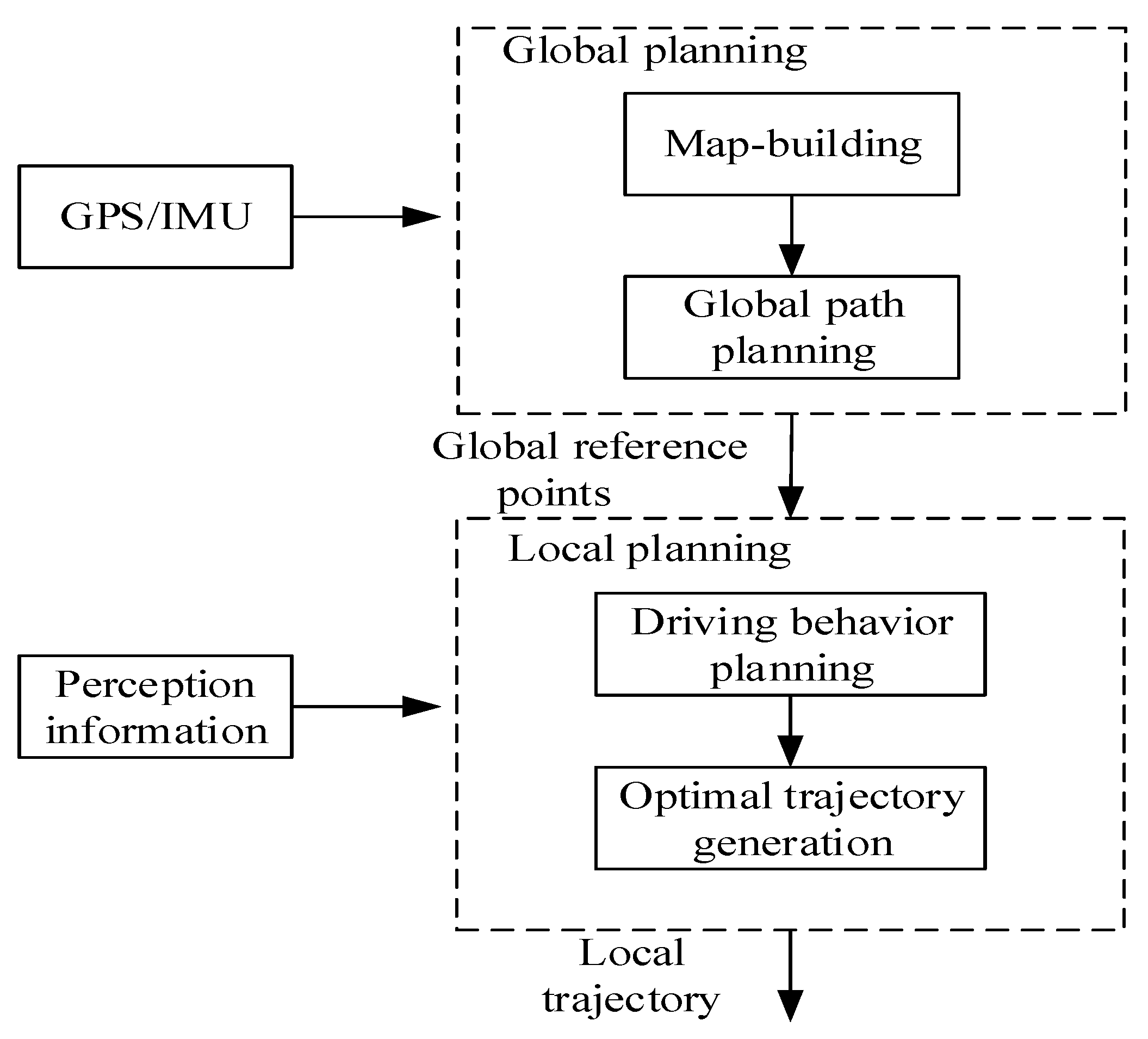
Path planning provides safe and reliable maneuvers under various driving environment, and it is the basis for autonomous vehicle to drive without human intervention. Figure 1 shows the framework of the path planning system. An integrated navigation system (GPS/IMU) provides vehicle speed, heading angle, and global position. The perception layer provides environmental information including static or dynamic obstacles and road information for path planning. Global planning is employed to find the optimal path from the current position to the destination in the high-precision GIS map form. Local planning plans appropriate driving behaviors and generates a smooth trajectory for the autonomous bus to follow the route.

In this paper, global planning is based on ArcGIS. Firstly, a high-precision GIS map is built according to original GPS data of path, which represents the road geometry. Then, the network analysis tool of ArcGIS is utilized to search for the optimal route in the high-precision map based on the current location which can be obtained by GPS/IMU.

Local planning contains two parts: driving behavior planning and optimal trajectory generation. Driving behavior planning imitates an experienced driver to give reasonable driving behaviors (e.g., lane changing, overtaking or following the vehicle ahead) based on perception information and global waypoints. Double-layer FSM (finite state machine) is proposed to execute a rule-based decision process under different driving scenarios. The trajectory generation module generates a safe and feasible path for autonomous bus. Here, a cubic polynomial is used to express optimal trajectory smoothly, which fully considers the kinetics and safety of the bus.

3. Map Building and Global Path Planning

Map-building is one of the core driverless technologies, which is crucial for positioning, navigation and control of autonomous electric bus. With the development of sensor technology, now accurate positioning of the lane through the GPS/IMU can be obtained. In this section, a high-precision map is constructed by ArcGIS.

ArcGIS offers a unique set of capabilities for applying location-based analysis to business practices. It is widely used for topographic map building [22] and map data analysis [23]. Here, a path is divided into two types which are the general path and special path, respectively. The path in GIS contains two parts: edge and node. All nodes are connected by the edges in order with no break point.

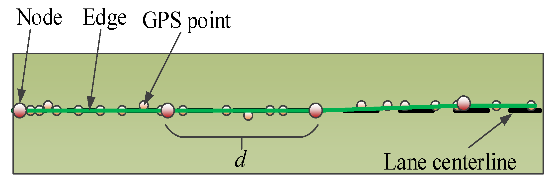
3.1. Map-Building in General Path

The general path refers to a straight lane and has no large turn. Original GPS data is imported to ArcGIS to build road network. The path in the GIS map is connected by edges in order. To reduce the amount number of GPS data, original data are filtered by setting the distance interval, which means the distance between nodes is d, as shown in Figure 2 (d ranges from 5 m to 10 m here).

3.2. Map-Building in Special Path

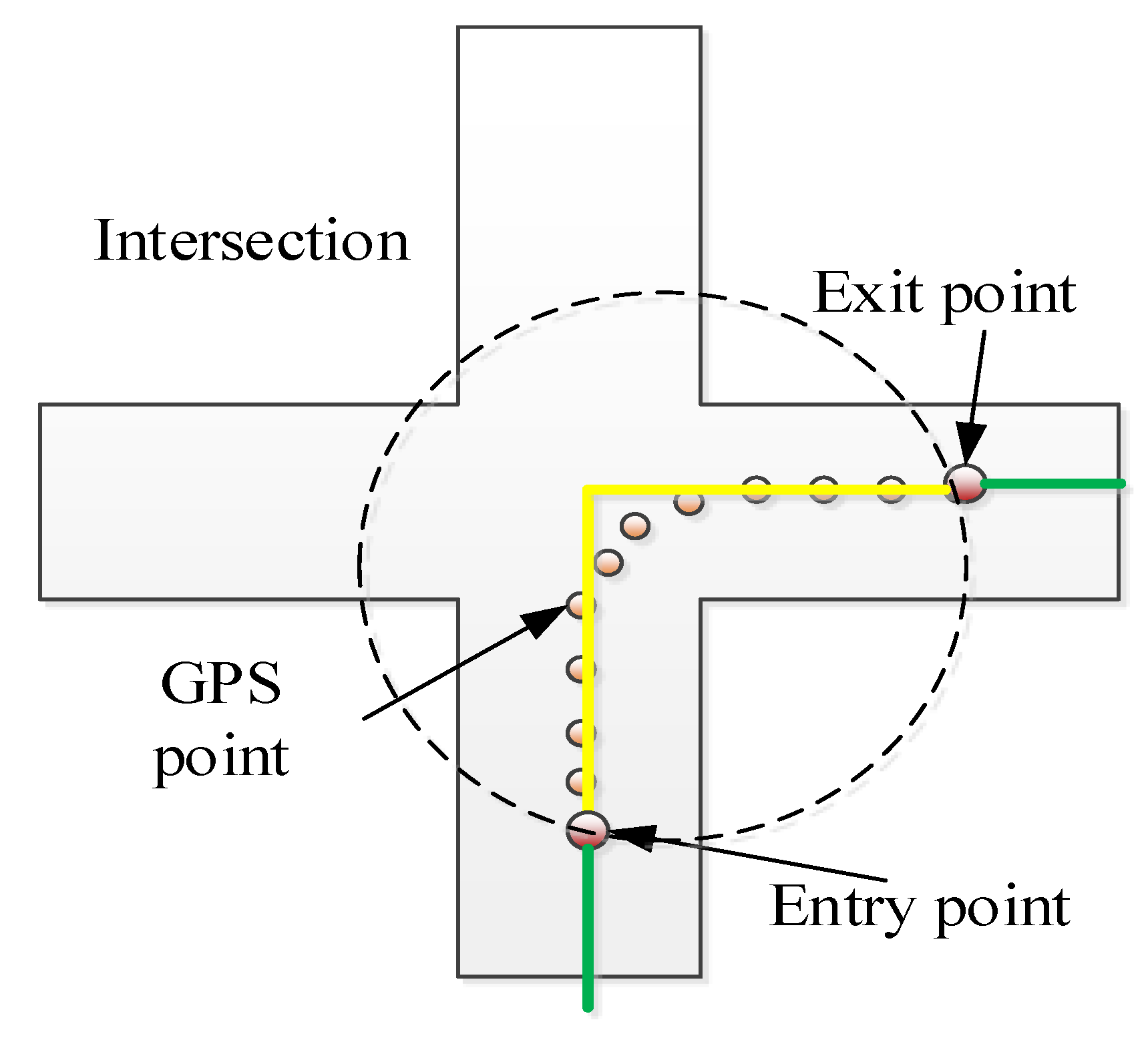
The special path refers to a path with a corner of a relatively large angle, such as intersections or ramps. Besides, there is no lane line can be detected by perception layer. The GPS data of special path is saved in special path database. Meanwhile, special mark points are respectively set on the two ends of the special path which are entry point and exit point. They are the key points to distinguish the general path and special path (Figure 3). The yellow line is only to keep path integrity in ArcGIS while the GPS points are the true global path.

Finally, two databases are established: GIS database and special path database. GIS database stores the road network information created by ArcGIS and the special path database stores GPS data of ramps or intersections.

3.3. Global Path Planning Based on ArcGIS

The road network map consists of two basic elements which are edges and nodes respectively, which forms a topology network structure. The direction of road, markers, and the other rules are all created in advance in the map. The global planning is to find the best path from the initial position to the destination based on such a network topology.

ArcGIS supports the network analysis very well based on the Geometric Network. So the global path planning is adopted by network analysis tool of ArcGIS. Then we can get the optimal path and all features (edges and nodes) of the path. The nodes in the global optimal path are the reference points for local planning. Besides, instead of planning one specific path to the destination, the global planning plans the path dynamically based on the current location of the bus.

3.4. Conversion of the Coordinate System

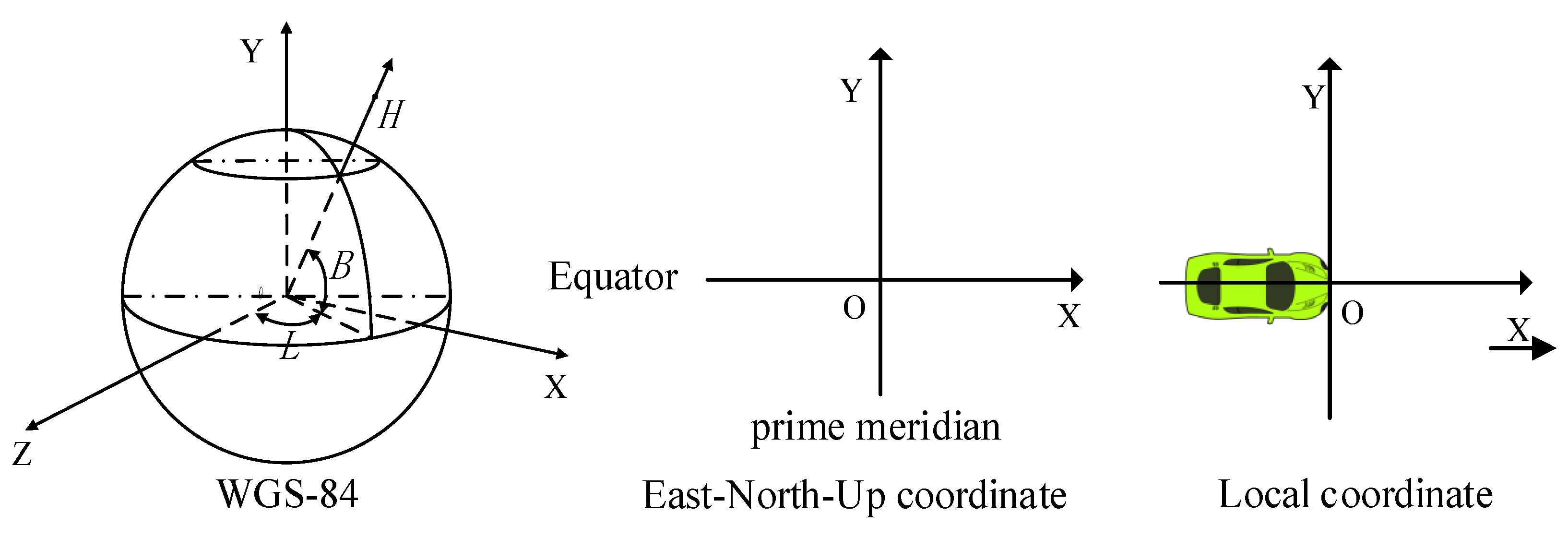
The built map is based on WGS-84 coordinate system, which is not suitable for local planning and control. WGS-84 coordinate system is transferred to local coordinate. Figure 4 displays the three types of coordinate systems. ‘East–north–up’ coordinates are a coordinate system where the X axis is lattitudinal, the Y axis is longitudinal, and the Z axis vertical.

$(B,L,H)$ represents the GPS data received from GPS/IMU which is the coordinate origin. B, L, and H represent longitude, latitude, and geodetic height in geocentric coordinate system. Then convert it to rectangular coordinate system $P(X_P,Y_P,Z_P)$ by Equations (1)–(3)

$$\left[\begin{array}{c}{X}_P\\ Y_P\\ Z_P\end{array}\right]=\left[\begin{array}{c}(R_n+H)\cos B\cos L\\ (R_n+H)\cos B\sin L\\ [(R_n+H)-e^2{R}_n]\sin B\end{array}\right]$$

(1)

$$R_n=a^2/{(a^2{\cos }^{2}B+b^2{\sin }^{2}B)}^{1/2}$$

(2)

$$e=(a^2-b^2)/a$$

(3)

where $R_n$ is radius of curvature in prime vertical and $e$ is the first eccentricity of ellipsoid. $a,b$ are semimajor axis of ellipsoid and semiminor axis of ellipsoid, respectively. $P(x_Q,y_Q,z_Q)$ is a point in rectangular coordinate. Then, the point $(x_{QP},y_{QP},z_{QP})$ in east–north–up coordinates is given by (4).

$$\left[\begin{array}{c}{x}_{\mathrm{QP}}\\ y_{\mathrm{QP}}\\ z_{\mathrm{QP}}\end{array}\right]=\left[\begin{array}{ccc}-\sin L& \cos L& 0\\ -\sin B\cos L& -\sin B\sin L& \cos B\\ \cos B\cos L& \cos B\sin L& \sin B\end{array}\right]\left[\begin{array}{c}{X}_{\mathrm{Q}}-X_{\mathrm{P}}\\ Y_{\mathrm{Q}}-Y_{\mathrm{P}}\\ Z_{\mathrm{Q}}-Z_{\mathrm{P}}\end{array}\right]$$

(4)

Finally, we can get the $(x^{\prime },y^{\prime })$ in local coordinate by (5) and provide the $(x^{\prime },y^{\prime })$ for local path planning.

$$\{\begin{array}{l}{x}^{\prime }=x_{op}*\cos yaw-y_{op}*\sin yaw\\ y^{\prime }=y_{op}*\cos yaw+x_{op}*\sin yaw\end{array}$$

(5)

where, $yaw$ is the heading angle of the bus.

4. Driving Behavior Planning Based on Double-Layer FSM

4.1. Top-Layer FSM Design

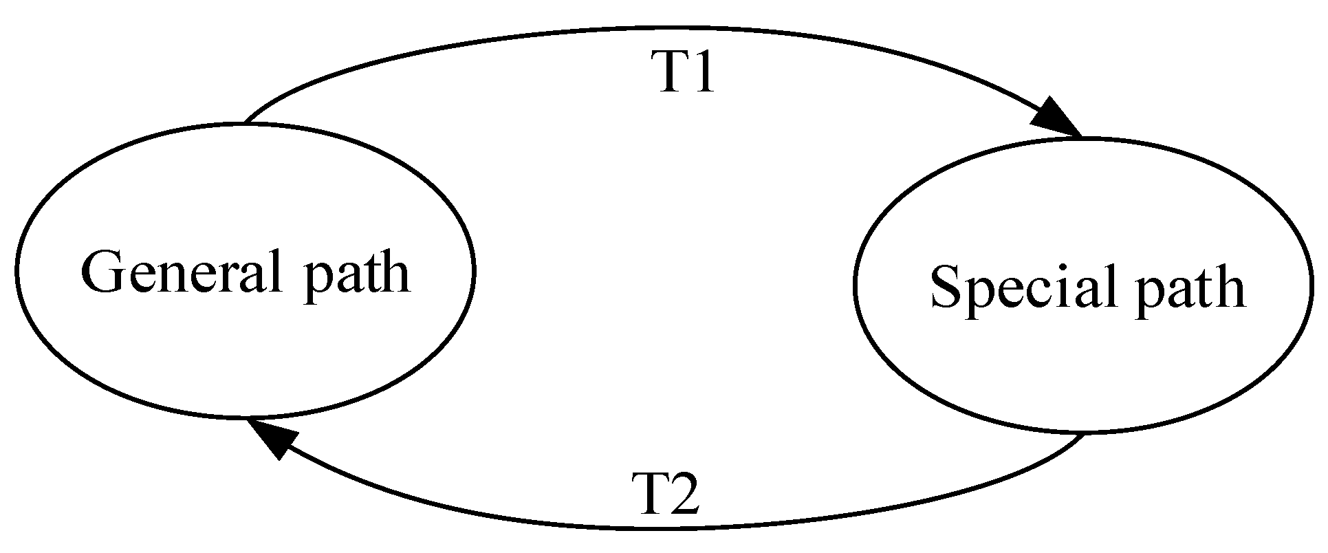
The map data of general path and special path comes from GIS database and special path database, respectively. In addition, the driving behavior under the two types of paths is different; for instance, overtaking is not allowed in special path so as to ensure safe driving for bus. Therefore, the state of top-layer FSM is devised as {general path (R1) and special path (R2)}. The type of road is distinguished by the entry point and exit point which are marked in global map (see Figure 3). The trigger events as follows:

T1: The bus passes the entry point.

T2: The bus passes the exit point.

Thus, the top-layer state transition shows in Figure 5.

4.2. Bottom-Layer FSM Design

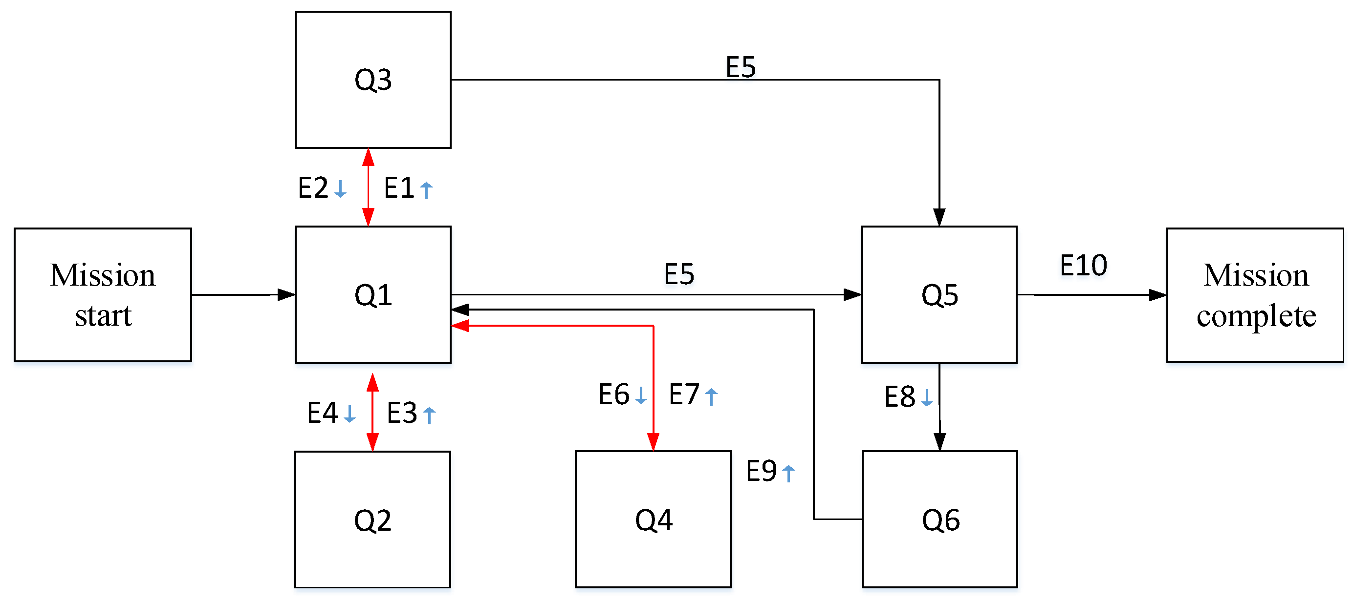
Driving scenarios for driverless bus are relatively simple and bus usually travels in a fixed route. In this section, the driving state set is designed as {structured driving (Q1), unstructured driving (Q2), following (Q3), overtaking (Q4), buffer adjustment (Q5), and special path (Q6)}. The corresponding external trigger events are devised based on the above states, which mainly divided into the following categories:

• E1/E2: The moving vehicle in front of the bus enters/disappears in detection area.
• E3/E4: The lane information from perception is valid/invalid.
• E5: The bus enters the buffered road.
• E6: The stationary obstacle in front of the bus enters in detection area.
• E7: The process of overtaking completes.
• E8: The bus enters the special path.
• E9: The bus finishes the special path.
• E10: The bus enters the area of destination.

According to the states and the trigger events, the bottom-layer FSM possesses six states, as shown in Figure 6. In our system, different behaviors also determine the local reference points which is used for trajectory generation.

• Structured driving: The bus drives in structured road and the lane recognition is valid. It is an initial state in the bottom-layer FSM. We mainly utilize the results of lane recognition in this stage to guide the bus to drive in this stage. So the local optimal reference points are generated by the results of lane detection.
• Following: It is a state that the autonomous bus can follow the vehicle ahead only when the lane detection is valid. The speed varies with the vehicle ahead.
• Overtaking: The autonomous bus overtakes the vehicle ahead which drives slowly (speed of the vehicle does not exceed 2 m/s) in this stage. It is divided into three steps: (a) lane change; (b) overtake; (c) lane return. Safe space is considered to avoid collisions with other vehicles. If $d_1<d_{th}$, the bus changes the lane ($d_1$ represents the distance between two vehicles, $d_{th}$ is the safe space). At this time, the local reference points are shifted from the current lane to another lane. The bus will return the lane again until it overtakes the vehicle and $d_1>d_{th}$.
• Buffer adjustment: It is an intermediate stage that the bus needs to adjust speed especially when the bus is around a ramp or intersection. The signs of enter and exit can be obtained from the global map.
• Special path: It is a stage after buffer adjustment and used to deal with special terrain such as intersections. The local reference points come from the special path database that is established in Section 3.2.
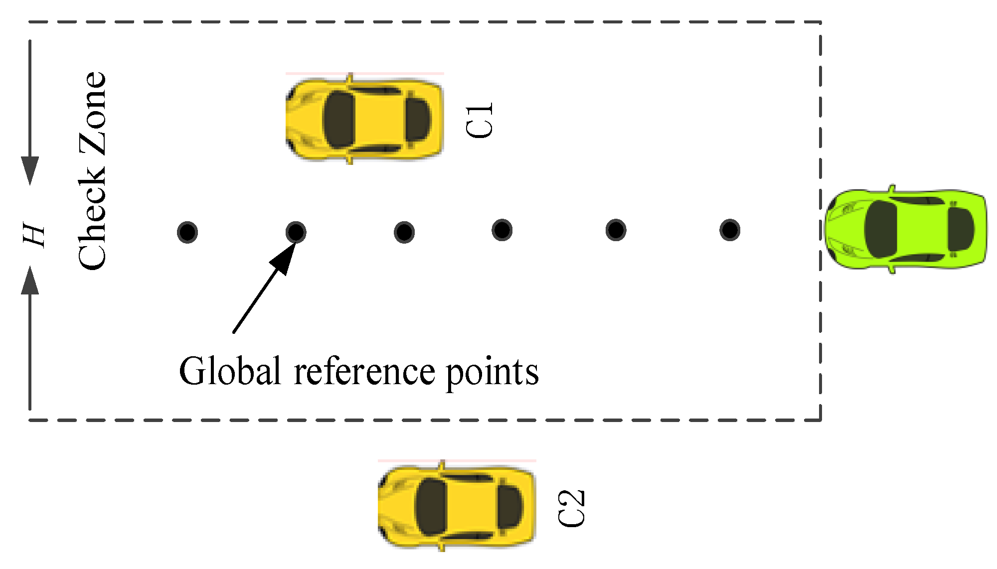
• Unstructured driving: Lane lines fail to be identified by perception layer in this stage. A check zone is set manually and detect the threaten obstacles in this area. Then check whether a dangerous obstacle exists in the check zone. For instance, in Figure 7, C1 is a threat for the bus while C2 is not.

5. Optimal Trajectory Generation

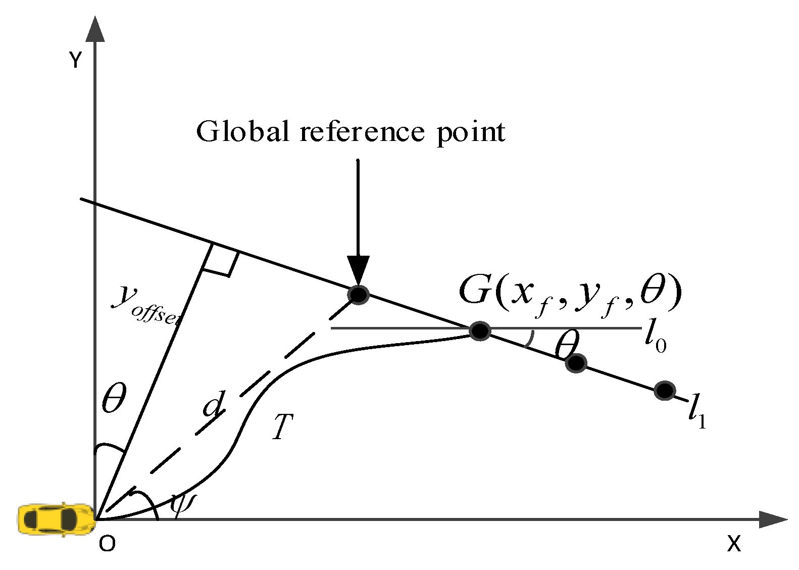
The global reference points cannot provide a feasible path for a bus to follow since they are usually sparse and unconstrained. It is proved that the mobile vehicle’s trajectory generation from start to end can be solved by using polynomial parameterizations [24]. To balance between computing complexity and constraints, cubic polynomial is applied to generate the optimal trajectory which is smooth and consistent with the bus kinetic constraints.

In Figure 8, $l_1$ is the fitted global path based on global reference points, the point $G(x_f,y_f,\theta )$ is a target point that is selected in global reference points to determine the expression of cubic polynomial. $\theta$ is the global desired heading, $T$ represents the cubic polynomial curve, $l_0$ is parallel to the X axis. The cubic polynomial can be written as

$$Y(X)=a_0+a_{1}x+a_2{x}^2+a_3{x}^3$$

(6)

where the coordinate system XOY is fixed with the center of the headstock. In the established coordinate system, the initial position is coordinate origin and initial heading of the bus is zero, that is, the constraints are expressed as

$$Y(0)=0$$

(7)

$$\raisebox{1ex}{$dY$}\!\left/ \!\raisebox{-1ex}{$dx$}\right.=0$$

(8)

combined with Equations (6)–(8), we can obtain the constant coefficients in (9).

$$a_0=a_1=0$$

(9)

To ensure the bus to track the global reference points finally, the trajectory in point G is tangent to $l_1$.The first derivative of cubic polynomial in the target point $G(x_f,y_f,\theta )$ i.e., the slope of $l_1$. Combined with Equations (6) and (9), the equation is expressed in (10)

$$\begin{array}{ll}{y}^{\prime }(x_f)& =2a_2{x}_f+3a_3{x}_f{}^2\\ & =\tan \theta \end{array}$$

(10)

Then, $y_{offset}$ (the offset of the target point) is written as (11).

$$y_{offset}=y_f\cos \theta +x_f\sin \theta$$

(11)

The target point $(x_f,y_f,\theta )$ is also a point on the cubic trajectory, so it satisfies the function

$$Y_f=a_2{x}_f{}^2+a_3{x}_f^3$$

(12)

combined with Equations (10)–(14) are obtained as

$$a_2=\frac{3y_{offset}}{x_f{}^2\cos \theta }-\frac{4\tan \theta }{x_f}$$

(13)

$$a_3=\frac{3\tan \theta }{x_f{}^2}-\frac{2y_{offset}}{x_f{}^3\cos \theta }$$

(14)

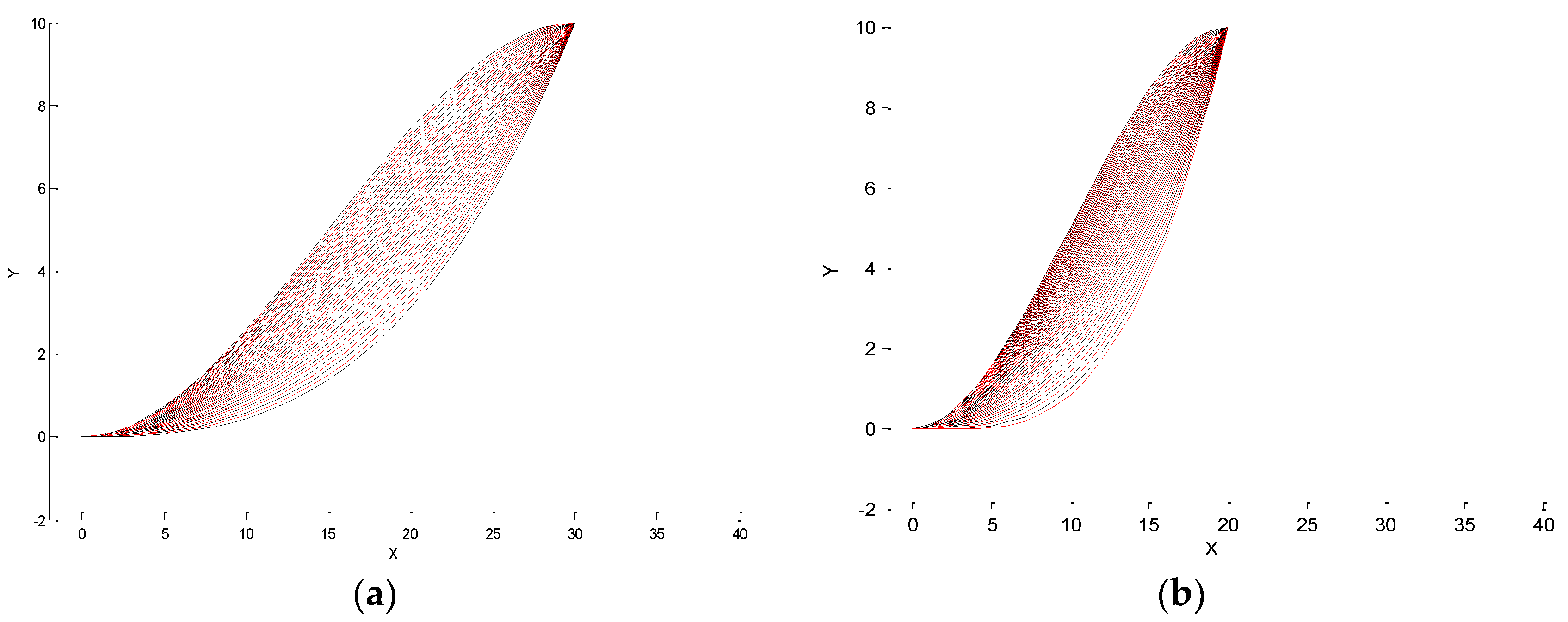
Therefore, the cubic polynomial is related to the target point $G(x_f,y_f,\theta )$, that is, different target points determine different trajectories. For instance, when the values of $x_f$ and $y_f$ are fixed but $\theta \in (0~{45}^{\circ })$, the trajectory clusters are showed in Figure 9a. Trajectory clusters of different target points are illustrated in Figure 9.

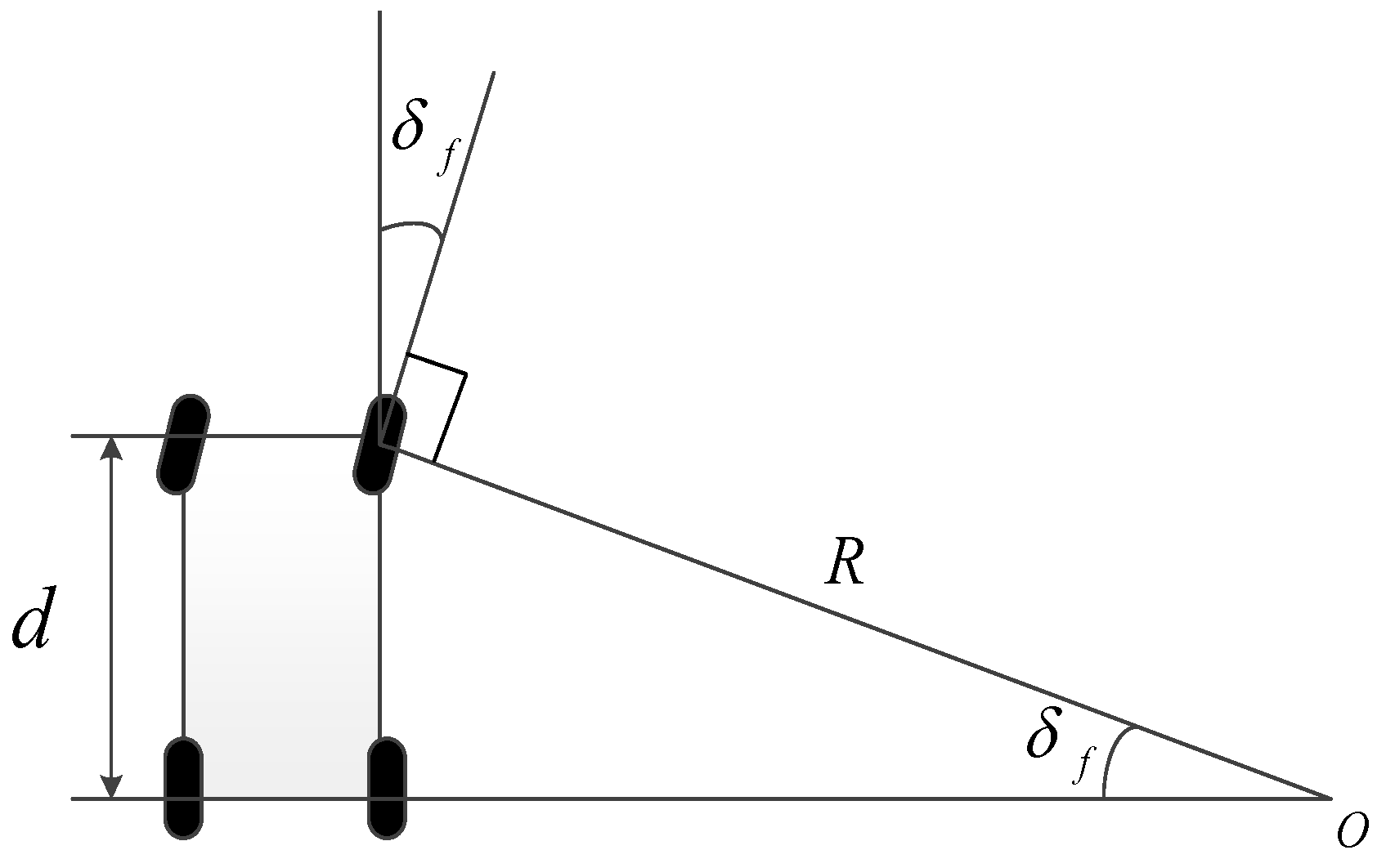
Therefore, an appropriate target point is essential for optimal trajectory. Besides, several constraints should be satisfied. On one hand, the maximum steering angle of the front wheel is limited for bus. The bus can travel through the target point with maximum front wheel angle. According to Figure 10, turning radius R can be written as (15).

$$R=d/\sin {\delta }_f$$

(15)

where ${\delta }_f$ is front wheel angle and d means the wheelbase. For the bus, the range of the front wheel $Rg\in [{\delta }_{f\min },{\delta }_{f\max }]$. From (15), the minimum turning radius is obtained by (16).

$$R_{\min }=d/\sin {\delta }_{f\max }$$

(16)

where ${\delta }_{f\max }$ is the maximum angle of front wheel.

On the other hand, the faster of the bus travels, the longer of trajectory should be. In this paper, a piecewise turning radius is defined by the equation

$$L_a=\{\begin{array}{cc}{R}_{\min }& v<v_{th}\\ R_{\min }+K_{la}v& v\ge v_{th}\end{array}$$

(17)

where $K_{la}$ is an adjusted coefficient, v represents the current speed, $v_{th}$ is a velocity threshold. Hence, the turning radius of a feasible target point is larger than $L_a$. Therefore, the optimal trajectory generation algorithm is described as Algorithm 1.

Algorithm 1. Optimal trajectory generation.

Input: Local optimal reference points Output: Trajectory equation Y(x) for I = 1; $R_i\ge L_a$ do 1: Calculate La according to the current speed. 2: Calculate the distance $d_i$ from coordinate point $(X_i,Y_i)$ (i = 1,2, ..., n,): $d_i=\sqrt{x_i{}^2+y_i{}^2}$. 3: Calculate the angel ${\psi }_i$ between the line and x-axis: ${\psi }_i=\arctan \left[\left(y_i-y_0\right)/(x_i-x_0)\right]$. 4: Calculate the lateral offset of $(X_i,Y_i)$. $y_{offset}(i)=d_i\times \sin ({\theta }_i-{\psi }_i)$. 5: Calculate minimum turning radius: $R_i=d_i{}^2/(2\ast y_{offset}(i))$. 6: end for 7: Calculate Y(x) according to $(X_i,Y_i,{\theta }_i)$, (8) and (9).

6. Simulation and Experiments

6.1. Simulation for Global Planning

Firstly, we built the high-precision map by importing GPS data to ArcGIS, the road network is shown in Figure 11a. Each path in the map contains several road attributes (e.g., length of the path, whether the path is one-way). The red arrow represents the definite direction of a road. Two types of database are built: GIS database and special path database. A special path database is utilized to deal with intersections or ramps. When the bus enters the special path, the bus gets global data from special database. Global optimal path (green line) was obtained from start point to destination by the network analysis tool of ArcGIS in Figure 11b. The optimal path can take the road attributes into account. The path 1→2→5 is shorter than path 1→2→3→4, but the path 5 is retrograde. Therefore, the optimal global path is 1→2→3→4.

6.2. Simulation for Local Planning

The driverless bus drives in a series of driving scenarios, including lane changing, lane keeping, and so on. Several typical driving scenarios are selected to test our method. The trajectory is generated by a cubic polynomial after the appropriate preview target point is determined based on the current state of the bus.

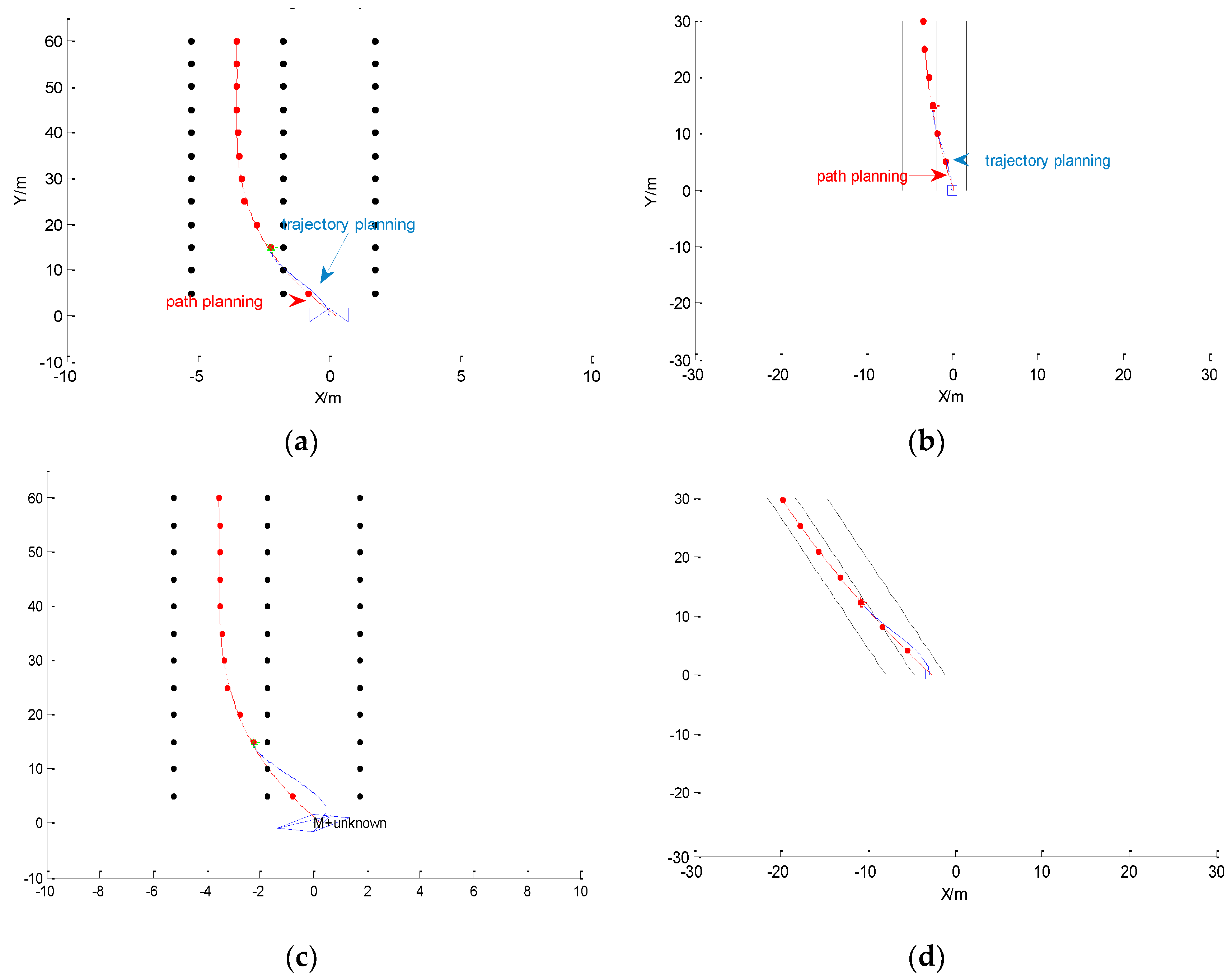
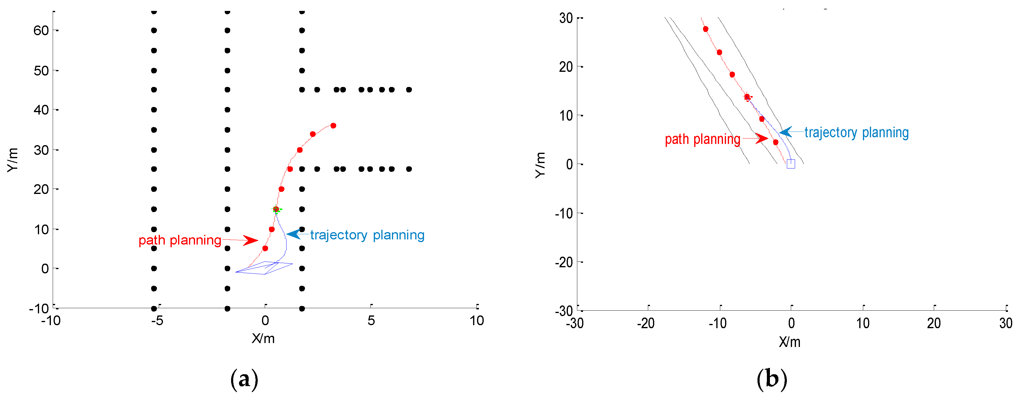
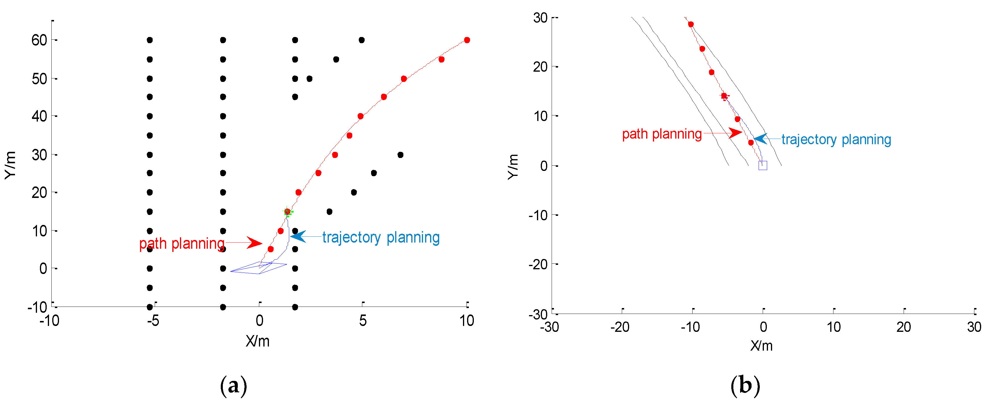
Figure 12 shows the planning results in global coordinate and local coordinate when the bus changed the lane. The red dots represent the global waypoints and the blue line represents the generated trajectory. Figure 12a,b display the trajectory when the bus moves forward and Figure 12c,d shows the trajectory when the bus towards the front right of the current lane. Despite having the same global waypoints and driving behavior, the two trajectories are different and they are adjusted to adapt the current heading of bus. Figure 13 describes the situation that the bus around a right turn and it exists heading error between the bus and global path. The local trajectory and the direction of the heading are tangent. It can ensure bus to track the trajectory smoothly and avoid a sharp turn although it exits large heading deviation. Similarly, Figure 14 displays the situation that the bus turns right around a ramp. The trajectory satisfies the constraint of vehicle kinematics and it is easy and feasible for a bus to track. Besides, all the results are displayed in global coordinates and local coordinates respectively.

Local planning can generate different trajectories according to the current direction of the bus. The initial direction of the trajectory is consistent with the driving direction, which is shown clearly in local coordinate. Furthermore, the generated trajectory by cubic polynomial is smooth and meets the bus kinematics.

6.3. Field Test

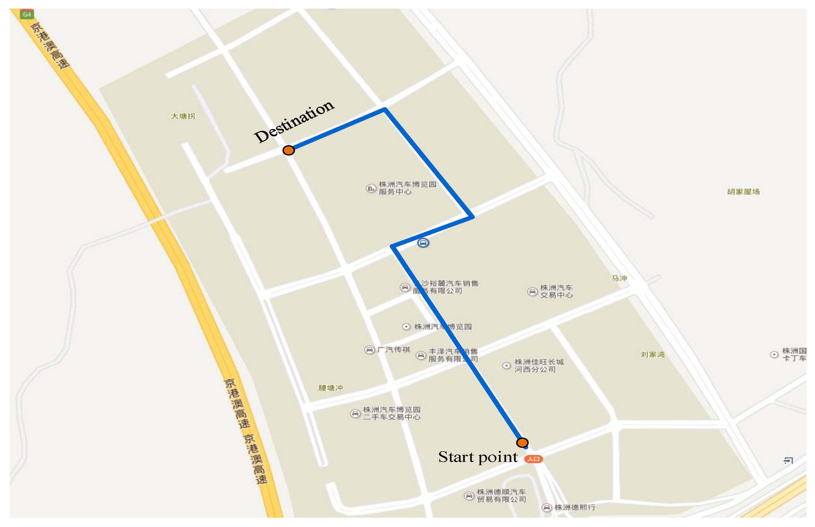
In order to evaluate the validity, stability, and reliability of the path planning system in real-world scenarios. The experimental area is an open road environment, including various vehicles passing in and out frequently. In this paper, we mainly focus on the method of path planning and trajectory generation, lateral and longitude controllers are not introduced here. In fact, the speed of the bus is adjusted constantly based on the information of obstacles, driving behaviors, curvature of the trajectory, etc. The blue line in Figure 15 is the global route of field test, which is in Zhuzhou, China.

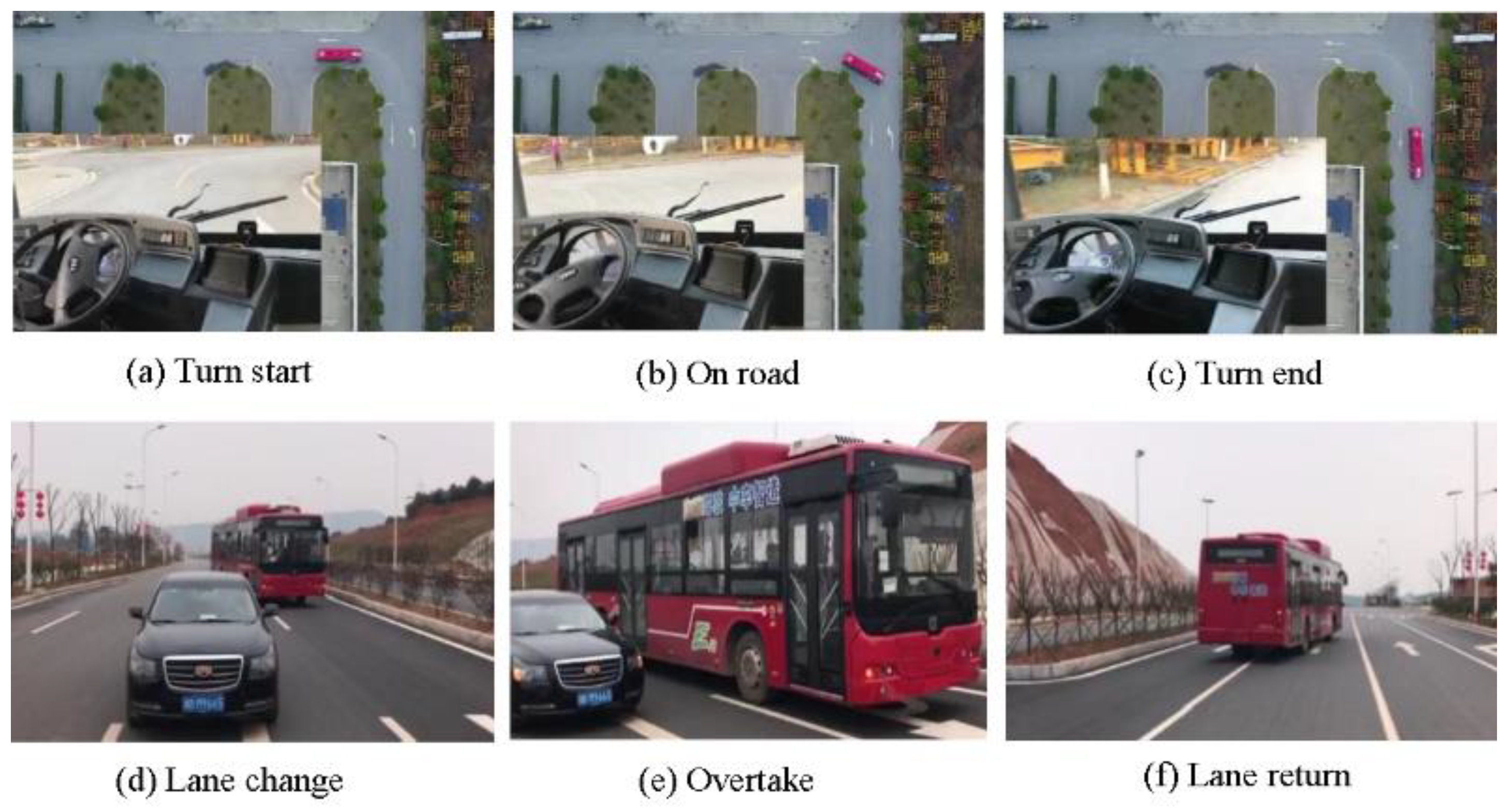
The autonomous driving platform is a 12 m electric bus with all kinds of sensors, including cameras, real-time kinematics GPS, inertial measurement unit (IMU), and laser scanners. The bus drove itself and completed the test successfully. Figure 16 shows the results and each picture is a snapshot from the driving videos, which are taken from inside, outside, or an aerial view of the bus. Figure 16a–c present the process of turning and Figure 16d–f show that the bus made decision by itself to overcome the car ahead.

7. Conclusions

This paper presents a framework of path planning for autonomous bus. The ArcGIS platform is applied for map-building and global path planning. It is flexible to add or edit road attributes (e.g., whether the path is one-way or accessible) in the high-precision map by ArcGIS. The global optimal path is planned from current position to destination in the map dynamically based on network analysis tool of ArcGIS. Besides, the local planning can infer a reasonable driving behavior according to the surroundings and generate a feasible and safe trajectory for autonomous bus. The local trajectory is expressed by cubic polynomial curve with constraints, and it meets the requirements of trajectory generation for bus and reduces computational complexity. Meanwhile, several simulations are devised to verify the proposed method. Furthermore, the bus successfully drives itself on the testing road that proves the validation and practicability of our system.

However, lots of advances are required for truly autonomous driving for busses. In future work, lots of field tests are conducted to verify our framework by driving relative complex scenarios. Besides, reinforcement learning is combined with FSM to predict driving behavior when an emergency scenario occurs.

References

- Tsai, C.C.; Huang, H.C.; Chan, C.K. Parallel Elite Genetic Algorithm and Its Application to Global Path Planning for Autonomous Robot Navigation. IEEE Trans. Ind. Electron. 2011, 58, 4813–4821. [Google Scholar] [CrossRef]
- Chen, Y.B.; Luo, G.C.; Mei, Y.S.; Yu, J.Q.; Su, X.L. UAV path planning using artificial potential field method updated by optimal control theory. Int. J. Syst. Sci. 2016, 47, 1407–1420. [Google Scholar] [CrossRef]
- Scheurer, C.; Zimmermann, U.E. Path planning method for palletizing tasks using workspace cell decomposition. In Proceedings of the IEEE International Conference on Robotics and Automation, Shanghai, China, 9–13 May 2011; pp. 1–4. [Google Scholar]
- Wesley, M.A. An algorithm for planning collision-free paths among polyhedral obstacles. ACM 1979, 22, 560–570. [Google Scholar]
- Takahashi, O.; Schilling, R.J. Motion planning in a plane using generalized Voronoi diagrams. IEEE Trans. Robot. Autom. 1989, 5, 143–150. [Google Scholar] [CrossRef]
- Wang, M.; Ganjineh, T.; Rojas, R. Action annotated trajectory generation for autonomous maneuvers on structured road networks. In Proceedings of the International Conference on Automation, Robotics and Applications, Wellington, New Zealand, 6–8 December 2011; pp. 67–72. [Google Scholar]
- Singh, H.; Bawa, S. Spatial data analysis with ArcGIS and MapReduce. In Proceedings of the International Conference on Computing, Communication and Automation IEEE, Noida, India, 29–30 April 2016. [Google Scholar]
- Chen, Y.; Su, F.; Shen, L.C. Improved ant colony algorithm based on PRM for UAV route planning. J. Syst. Simul. 2009, 21, 1569–1658. [Google Scholar]
- Amato, N.M.; Wu, Y. A randomized roadmap method for path and manipulation planning. In Proceedings of the IEEE International Conference on Robotics and Automation, Minneapolis, MN, USA, 22–28 April 1996; Volume 1, pp. 113–120. [Google Scholar]
- Wang, F.; Zhu, Z. Global Path Planning of Wheeled Robots Using a Multi-Objective Memetic Algorithm. Integr. Comput. Aided Eng. 2015, 22, 387–404. [Google Scholar]
- Tang, B.; Zhu, Z.; Luo, J. A convergence-guaranteed particle swarm optimization method for mobile robot global path planning. Assem. Autom. 2017, 37, 114–129. [Google Scholar] [CrossRef]
- Baker, C.R.; Dolan, J.M. Street smarts for boss. IEEE Robot. Autom. Mag. 2009, 16, 78–87. [Google Scholar] [CrossRef]
- Wang, X.Y.; Yang, X.Y. Study on decision mechanism of driving behavior based on decision tree. J. Syst. Simul. 2008, 20, 414–415. [Google Scholar]
- Furda, A.; Vlacic, L. Enabling Safe Autonomous Driving in Real-World City Traffic Using Multiple Criteria Decision Making. IEEE Intell. Transp. Syst. Mag. 2011, 3, 4–17. [Google Scholar] [CrossRef] [Green Version]
- Galceran, E.; Cunningham, A.G.; Eustice, R.M.; Olson, E. Multipolicy decision-making for autonomous driving via changepoint-based behavior prediction: Theory and experiment. Auton. Robot. 2017, 41, 1367–1382. [Google Scholar] [CrossRef]
- Beaucorps, P.D.; Streubel, T.; Verroust-Blondet, A.; Nashashibi, F.; Bradai, B.; Resende, P. Decision-making for automated vehicles at intersections adapting human-like behavior. In Proceedings of the Intelligent Vehicles Symposium, Los Angeles, CA, USA, 11–14 June 2017. [Google Scholar]
- Jo, K.; Kim, J.; Kim, D.; Jang, C.; Sunwoo, M. Development of Autonomous Car—Part II: A Case Study on the Implementation of an Autonomous Driving System Based on Distributed Architecture. IEEE Trans. Ind. Electron. 2015, 62, 5119–5132. [Google Scholar] [CrossRef]
- Montemerlo, M.; Becker, J.; Bhat, S.; Dahlkamp, H.; Dolgov, D.; Ettinger, S.; Haehnel, D.; Hilden, T.; Hoffmann, G.; Huhnke, B.; et al. Junior: The Stanford Entry in the Urban Challenge. J. Field Robot. 2008, 25, 569–597. [Google Scholar] [CrossRef]
- Chen, C.; Yu-Qing, H.E.; Chun-Guang, B.U.; Han, J.D. Feasible Trajectory Generation for Autonomous Vehicles Based on Quartic Bézier Curve. Acta Autom. Sin. 2015, 41, 486–496. [Google Scholar]
- Rodriguez, L.; Balampanis, F.; Cobano, J.A.; Maza, I.; Ollero, A. Energy-efficient trajectory generation with spline curves considering environmental and dynamic constraints for small UAS. In Proceedings of the IEEE/RSJ International Conference on Intelligent Robots and Systems, Vancouver, BC, Canada, 24–28 September 2017; pp. 1739–1745. [Google Scholar]
- Cong, Y.; Sawodny, O.; Chen, H.; Zimmermann, J.; Lutz, A. Motion planning for an autonomous vehicle driving on motorways by using flatness properties. In Proceedings of the IEEE International Conference on Control Applications, Yokohama, Japan, 8–10 September 2010; pp. 908–913. [Google Scholar]
- Guan, Z.; Huang, S.; Rong, J. Experimental Analysis of the Geomorphic Hill Shading Map Production Based on ArcGIS. J. Geomat. 2017, 42, 101–103. [Google Scholar]
- Han, L.; Do, Q.H.; Mita, S. Unified path planner for parking an autonomous vehicle based on RRT. In Proceedings of the IEEE International Conference on Robotics and Automation, Shanghai, China, 9–13 May 2011; pp. 5622–5627. [Google Scholar]
- Qu, Z.; Wang, J.; Plaisted, C.E. A new analytical solution to mobile robot trajectory generation in the presence of moving obstacles. IEEE Trans. Robot. 2004, 20, 978–993. [Google Scholar] [CrossRef]
Figure 1.
Framework of path planning for autonomous bus.