A Collision Avoidance Strategy Based on Entropy-Increasing Risk Perception in a Vehicle–Pedestrian-Integrated Reaction Space

Abstract

Ensuring pedestrian safety is one of the most significant challenges for autonomous driving systems in urban scenarios due to the non-cooperative and unpredictable nature of pedestrian movements. To tackle this problem, firstly, we propose a collision avoidance strategy based on entropy-increasing risk perception in a vehicle–pedestrian reaction space. Our approach combines a limited range of reaction space regions with entropy to quantify the risk of pedestrian–vehicle collision. Then, multi-vehicle candidate trajectories are generated using the path and speed sequence method, and the uncertain states of pedestrians are predicted based on the social force model and Markov model accordingly. Finally, to determine the optimal collision avoidance trajectory, we use quantitative reaction-space entropy as a new “cost function” to measure potential risk and perform multi-objective trajectory optimization based on the elitist non-dominated-sorting genetic algorithm region-focused (NSGA-RF) approach. Simulation results show that our proposed strategy can enhance the safety of the planned trajectory interaction between vehicles and pedestrians for autonomous driving under normal and emergency conditions.

1. Introduction

As typical vulnerable road users, pedestrians’ safety is a critical transport concern, as there is a high occurrence of vehicle–pedestrian collision incidents due to the non-cooperative and unpredictable nature of pedestrian movements. For this reason, researchers have been working diligently to develop more effective vehicle–pedestrian interaction prediction and anti-collision mechanisms. Many researchers have conducted extensive research in the field of autonomous-driving collision avoidance. Model predictive control (MPC) has an advantage in vehicle dynamics as it deals with multiple constraints of control objectives input depending on the optimization algorithms [1]. Therefore, collision avoidance control systems based on MPC have received substantial attention. For example, in [2], H. Li, et al. presented a control strategy that integrates four-wheel steering and utilizes adaptive model predictive control (AMPC) to implement collision avoidance, and in [3], S. Cheng et al. divided the driving state into three categories and adjusted the weight of the MPC cost function based on different driving states. Meanwhile, advancements in computer technology and artificial intelligence (AI) have accelerated the research on collision avoidance. Early models such as the time-to-collision acceleration model [4] and its subsequent improvements [5,6] incorporated probability theory to predict the likelihood of collision avoidance with obstacles [7,8]. Utilizing probabilistic models such as the Bayesian network [9] and the Markov model [10] provided trajectory routes that were generated through a combination of path-planning algorithms and applied to various road-interaction scenarios. Some of the primary path-planning algorithms included A*, polynomial, and ant-colony algorithms [11,12,13], while others utilized curve fitting [14]. Additionally, researchers have proposed extracting contextual information from smartphones and wireless networks, such as Wi-Fi, in developing collision avoidance methods and related security systems [15,16,17]. Other studies analyzed the constraints between different variables, such as vehicles, bicycles, pedestrians, road conditions, and vehicle speeds, and developed corresponding theoretical methods [18,19,20]. Then, with the rapid advancement of communications technology, multi-vehicle cooperative collision avoidance was proposed: for example, multiple-vehicle cooperation and collision avoidance (MVCCA) [21] and reinforced cooperative autonomous-vehicle collision avoidance (RACE) [22]. However, it is important to note that these studies were primarily concentrated on vehicle decision-making and trajectory action, with little attention paid to the unpredictability of pedestrian motion. Collision avoidance research must give consideration to both pedestrians and vehicles as they are major participants within a traffic system. With AI algorithms, some studies utilized convolutional neural networks to predict behavior trajectories [23,24,25,26], while others used deep reinforcement-learning algorithms to improve the accuracy of trajectory predictions [27,28,29,30,31]. Pedestrian behavior on the road is highly random, significantly increasing the challenge of collision avoidance, especially when uncertain factors arise during emergencies and increase the risk of collisions. In [32], researchers divided behavior models without interactions into unstructured walking models with known goals and behavior prediction with unknown goals. Because pedestrians exhibit non-cooperative behavior, there is a need to further improve the degree of coincidence between predicted and actual traffic rule outcomes [33,34], especially in emergency situations.

To tackle the above challenges, we propose an active collision avoidance strategy for autonomous vehicles that incorporates risk perception constructed through the integration of reaction-space entropy. This results in a series of trajectories generated by combining path and speed planning while considering pedestrian–vehicle interaction through a probability model to predict pedestrian positions. Stability and safety requirements are combined with quantified reaction-space entropy to be used as cost functions for trajectory evaluation. Lastly, a series of simulations are performed to validate the effectiveness of the proposed collision avoidance strategy. Figure 1 illustrates the specific architecture process.

Our main contributions are summarized as follows:

(1)

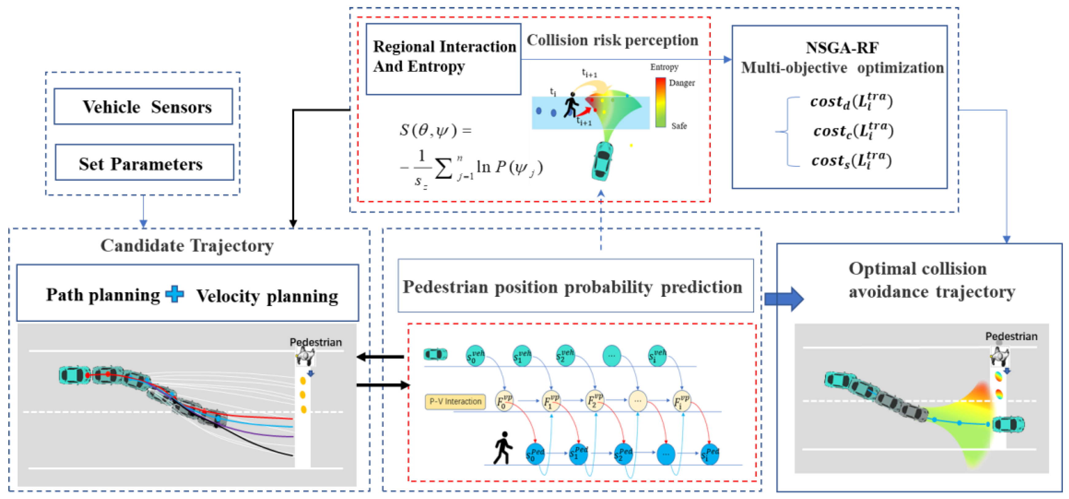
A collision avoidance strategy based on reaction-space regions with entropy-increasing risk perception is proposed.

(2)

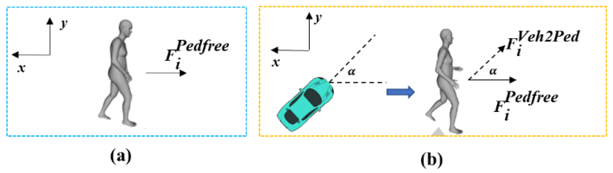
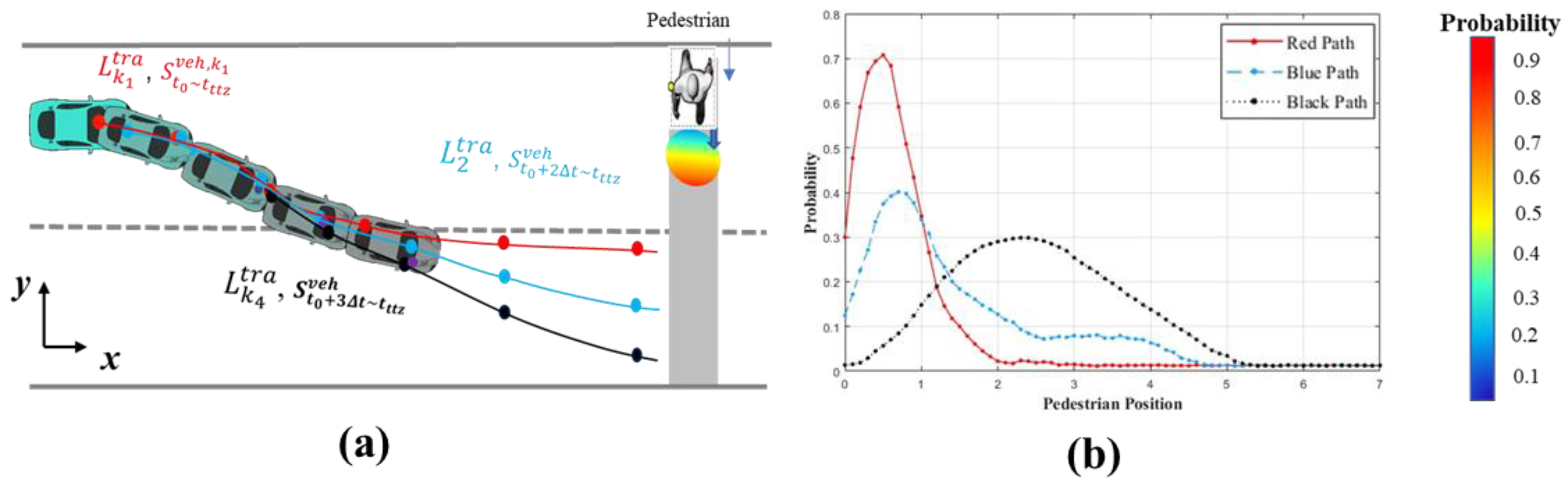
Path and speed sequences are adopted to generate candidate trajectories while predicting the uncertain states of pedestrians based on the social force model and the Markov model.

(3)

Response-space entropy is used as a new cost function to measure the collision risk and to optimize multi-target trajectories while considering factors of entropy, safety, and stability.

This paper is divided into seven sections. The current status of pedestrian collision avoidance trajectories in autonomous driving systems is described in Section 1. The representation of the reaction space and the quantification of entropy are introduced in Section 2. Section 3 generates candidate trajectories through path planning and speed planning. In Section 4, a vehicle–pedestrian interaction model is constructed by integrating the reaction space with predictions of pedestrian positions. Section 5 introduces the selection of the optimal trajectory using the NSGA-RF algorithm through cost functions. The simulation and result analyses are presented in Section 6. Section 7 presents the conclusion and suggests future directions from this paper.

2. Related Work

Collision avoidance mechanisms are largely influenced by the timing and strategy of decision-making. This involves an increasing amount of cognitive processing for decision-making due to the complexity of changes in the driving environment. To simplify this challenge, we use a vehicle–pedestrian reaction space and the entropy quantification method to compute the collision risk map.

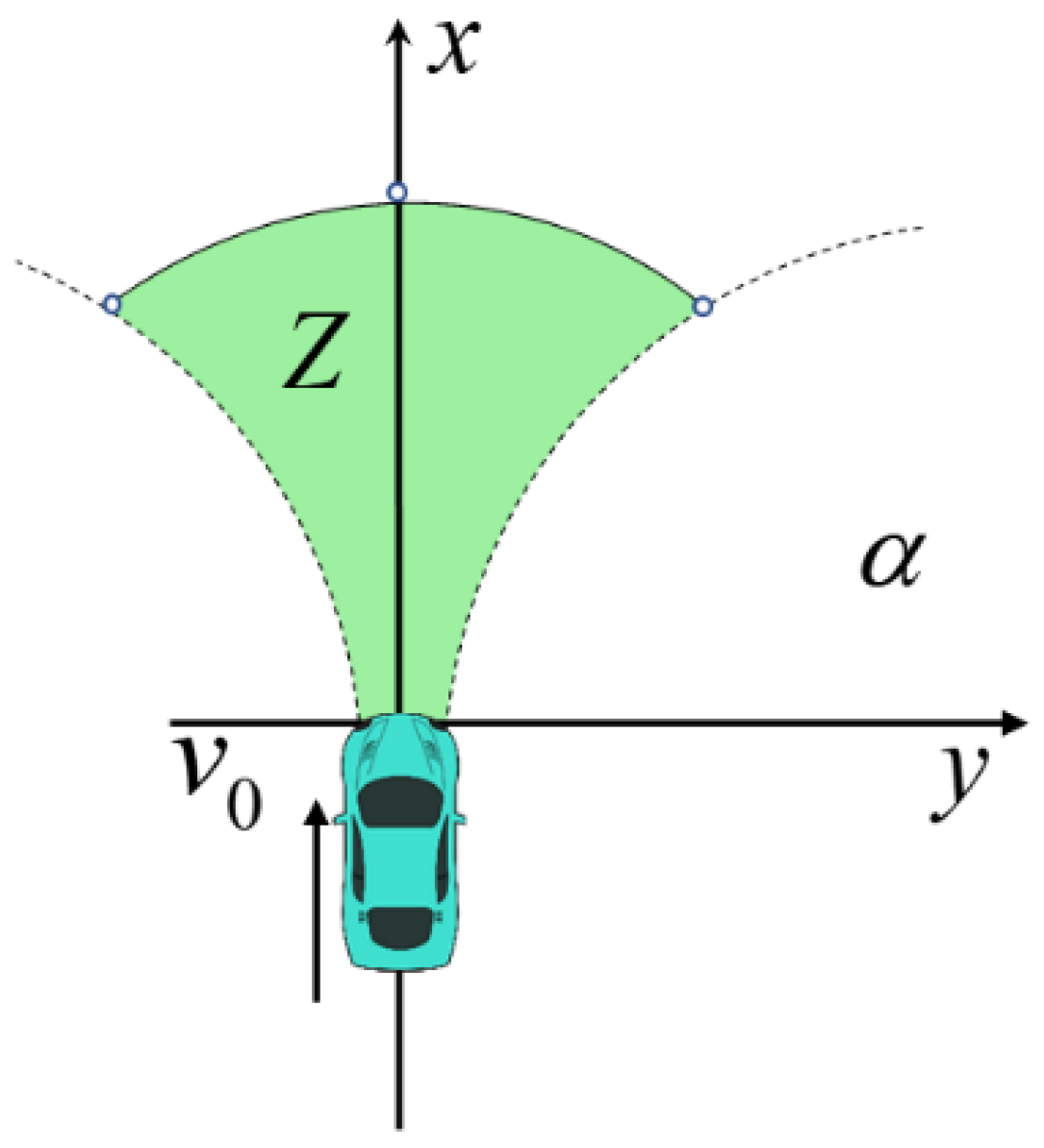
2.1. Reaction Space Constraints

To ensure that autonomous vehicles have sufficient time to process information and provide appropriate feedback, the response space description must accurately reflect the current driving state and situation in time. In [35,36], the reaction space $Z$ has been defined as an area that the vehicle can reach within a future time period of $k$ seconds. The range of this space is determined both by the position of the vehicle within $t$ seconds in the future and by its theoretical state parameters. As shown in Figure 2, the curve boundary of the reaction space is determined by the maximum centrifugal acceleration $a_c$ that is produced as a result of vehicle resistance. The space appears as a closed area when the vehicle is operating at a constant speed without major state changes, thereby indicating that the vehicle is not interacting with other road users. In this area, the vehicle is contained within the dotted line corresponding to its radius at a consistent speed, while the outer solid line represents the circle formed by the distance radius along the x-axis during the time period $t$. The mathematical expression of the dotted line in the coordinate system can be given as

$$\begin{array}{l}x=\frac{v_0^2}{f_{\max }g}\cos (\frac{f_{\max }gt}{v_0})\\ y=\frac{B}{2}+\frac{v_0^2}{f_{\max }g}\sin (\frac{f_{\max }gt}{v_0})\end{array}$$

(1)

where $v_0$ is the initial speed, with units of $\mathrm{m}/\mathrm{s}$; $g$ corresponds to the gravitational acceleration, with units of ${\mathrm{m}/\mathrm{s}}^2$; $B$ is the width of the vehicle, with units of $\mathrm{m}$; and $f_{\max }$ is the maximum achievable friction coefficient between the tire and the road. The radius forming the solid part of the circle can be described as

$$\begin{array}{l}{x}_r={\displaystyle {\int }_0^T(f_{\max }g+a_r)tdt}\\ y_{\mathrm{r}}=0\end{array}$$

(2)

where $a_r$ is the instantaneous deceleration of the vehicle, with units of ${\mathrm{m}/\mathrm{s}}^2$; $t$ and $T$, respectively, correspond to the time when the vehicle speed becomes zero and the time when the vehicle is in a certain position at a certain time in the future. Here, $T$ can be assumed as the time when the vehicle arrives at the predicted area of a potential collision with pedestrians, during which the speed of the vehicle may not be zero.

In summary, we can obtain the following closed reaction space $Z$, i.e., where all positions inside the area are accessible to the vehicle.

2.2. Entropy Quantification and Collision Risk Perception

The regional interaction of road users in an autonomous driving system is a dynamic and complex process. The nature of collision depends on the state of road users in the construction of the system and the dynamic sequence between them, transforming it into the entropy theory. The concept of entropy was proposed by the German physicist Rudolf Clausius in 1867 [37]. Entropy can be used to measure the level of organization and chaos, consistency and diversity, and disorder in different systems and fields of science. In the macroscopic state of thermodynamics, entropy represents the degree of irregular arrangement between particles in a system composed of a large number of particles. The more “chaotic” the system is, the greater the entropy will be. It means that if the macroscopic state of a system is specified, the value of entropy can be determined. The application of entropy involves exploring the complexity of urban construction or illustrating its use for monitoring and management in urban sprawl research [38]. However, entropy is rarely applied to measure collision risk in a transportation system.

Entropy is a measure of chaos in a system, which can be defined as the product of the probability of a specific system entity state and the quantity defining the physical properties of the system, i.e.,

$$S=-k{\displaystyle {\sum }_{i=1}^{n}p(x_i)\ln }p(x_i)$$

(3)

where $p(x_i)$ is the probability function that the system entity appears in a specific state $x_i$, $n$ is the total number of possible states, and $k$ is a constant defining the physical properties of the system. To combine the actual situation, we define the following parameters:

(1)

$\theta$ is a vector representing the existence of the entity in the constrained reaction-space area.

(2)

$P({\theta }_i)$ is the probability of the existence of the ith entity, referring to the ith pedestrian involved in the vehicle reaction space.

(3)

${\psi }_j$ is defined as the $j$ unique interaction vector between the ith entity (pedestrian) and the vehicle.

(4)

$P({\psi }_j)$ is the probability of each vector $j$ interaction, which is considered as the probability of collision of the pedestrian interacting with the vehicle at different positions in the reaction space.

It should be noted that when there is no pedestrian in the reaction space, the probability of $P({\theta }_i)$ is zero, and the probability of interaction between the corresponding entities $P({\psi }_j)$ is also zero. In summary, the reaction-space entropy we described can be expressed as

$$S(\theta ,\psi )=-\frac{1}{k}{\displaystyle {\sum }_{i=1}^m{\displaystyle {\sum }_{j=1}^n(P({\theta }_i)\ln P({\theta }_i)+P({\psi }_i)\ln P({\psi }_j))}}$$

(4)

It should be noted that this paper considers only one pedestrian in the reaction space, which refers to the condition in which $P({\theta }_i)=1$, representing the entropy of the reaction space of the potential collision interaction behavior between the vehicle and the pedestrian. The expression can be simplified as

$$S(\theta ,\psi )=-\frac{1}{k}{\displaystyle {\sum }_{j=1}^n\ln P({\psi }_j)}$$

(5)

At this time, $P({\psi }_j)$ can be defined as the probability of pedestrians appearing in different positions in the reaction space at the moment of collision. Under this condition, the value of the response-space entropy based on the predicted pedestrian position should be an uncertainty constant greater than or equal to zero. After selecting a specific vehicle trajectory in the generated candidate trajectory sequence, the position and probability of the corresponding pedestrian in the collision prediction area under this trajectory are inferred from considering the interaction between the vehicle and the pedestrian.

The area $S_z$ of the reaction space at the corresponding time can be used to replace the calculation constant $k$ in (5). Then, the entropy of the system indicating the risk of the pedestrian–vehicle collision in this state can be obtained as

$$S(\theta ,\psi )=-\frac{1}{s_z}{\displaystyle {\sum }_{j=1}^n\ln P({\psi }_j)}$$

(6)

Under different trajectories, the location probabilities of pedestrians, as well as the entropy of the system, will be different. The reaction-space entropy of the system can be used as a cost function to evaluate the candidate trajectories, which help to evaluate the optimal trajectory when combined with multi-objective optimization.

3. Generation of Candidate Trajectories

This section will explain the path-planning method based on the fifth-order polynomial [12] to fully consider the continuity information of vehicle speed, acceleration, and pedestrian uncertain dynamic factors. It is necessary to realize that the speed planning of the vehicle is also very important. To ensure the safety of the trajectory, i.e., no collisions, the speed of the vehicle must be stable, and the selection of the steering angle should be smoother.

3.1. Path Planning

In the path-planning process, the state of the vehicle planned by candidate trajectory $l$ at moment $i$ can be described as

$${{\displaystyle s}}_i^{veh,l}=({{\displaystyle x}}_i^{veh},{{\displaystyle y}}_i^{veh},{{\displaystyle v}}_i^{veh},{{\displaystyle \alpha }}_i^{veh})$$

(7)

where $x_i^{veh}$ and $y_i^{veh}$ refer to the coordinates of the vehicle’s position at moment $i$, while $v_i^{veh}$ and ${\alpha }_i^{veh}$, respectively, correspond to the velocity and the angle between the vehicle’s trajectory and the y-axis at moment $i$.

During the dynamic interaction between pedestrians and vehicles on urban roads, although it is challenging, and even impossible, to precisely predict the precise future motion of transportation vehicles, it is feasible to estimate their future approximate motion over a short period of time by utilizing a set of potential trajectories [39]. In addition, the continuous path generated by the planning should be as smooth as possible relative to the previous position point, ensuring safety while meeting the boundary constraints. The quintic polynomial path-planning method can satisfy the constraints of speed, acceleration, displacement, and other conditions related to each trajectory point for continuous re-planning. The specific path-planning equation incorporating the vehicle model and the parameters defined above can be given as

$$\begin{array}{l}{\dot{x}}_i^{veh}=v_i^{veh}\cos {\theta }_i^{veh}\\ {\dot{y}}_i^{veh}=v_i^{veh}\sin {\theta }_i^{veh}\\ {\dot{\theta }}_i^{veh}=v_i^{veh}{k}_{\lim }\end{array}$$

(8)

where $\theta$ and $k$ are, respectively, the heading angle of the vehicle and the curvature of the candidate path at the current moment, and $k_{\lim }$ is the limit value of the steering limit imposed by the vehicle.

$$k=\frac{{\dot{x}}_i^{veh}{\ddot{y}}_i^{veh}-{\ddot{x}}_i^{veh}{\dot{y}}_i^{veh}}{{({({\dot{x}}_i^{veh})}^2+{({\dot{y}}_i^{veh})}^2)}^{\frac{3}{2}}}\le k_{\lim }$$

(9)

The position information of the above-mentioned fifth-degree polynomial path-planning algorithm in the Cartesian coordinate system conforms to the following:

$$y(x_i^{veh})=\{\begin{array}{c}{\displaystyle {\sum }_{\tau =0}^5{{\displaystyle a}}_{\tau }{{\displaystyle x}}^{\tau },(x\in [0,x_{final}))}\\ y_{final},(x\ge x_{final})\end{array}$$

(10)

where $a_{\tau }$ is the polynomial equation coefficient, while $x_{final}$ and $y_{final}$ are the horizontal and vertical position parameters of the final point of the collision-avoidance planning trajectory, which are satisfied by

$$\begin{array}{l}y(0)=y_i\\ {\dot{y}}_{x=0}=\tan {\theta }_i^{veh}\\ {\ddot{y}}_{x=0}=\frac{1}{{\ddot{x}}_{(t)}}{[{\ddot{y}}_{(t)}-\frac{{\ddot{x}}_{(t)}{\dot{y}}_{(t)}}{{\dot{x}}_{(t)}}]}_{t=0}\\ \dot{y}(x_{final})=0\\ \ddot{y}(x_{final})=0\end{array}$$

(11)

where $y_i$ represents the initial coordinate position along the y-axis of the coordinate system established in a planning cycle, ${\theta }_i^{veh}$ is the initial heading angle of the vehicle in the corresponding cycle, $\dot{x}(t)$ and $\ddot{x}(t)$ are the corresponding longitudinal velocity and the acceleration of vehicle, and $\dot{y}(t)$ and $\ddot{y}(t)$ are the lateral velocity and acceleration in the established coordinate system. In practice, these parameters can be directly obtained by the onboard sensory equipment, and these are not studied in this paper. In the actual simulation experiment, the relevant data can be assigned according to the specific situation.

Figure 3 shows the process of using a fifth-degree polynomial for continuous path-planning updates in real time. When the autonomous vehicle enters the range of sensors at moment $t_0$, it will obtain the state parameters about the vehicle and pedestrian. After that, a series of alternative paths will be planned, and a temporary trajectory that best meets the constraints, $L_{k_1}^{tra}$, will be determined. Then, the subsequent cycles will be globally re-planned based on the data of the previous cycle until the interaction process of collision avoidance is completed. Among them, $L_{k_1}^{tra}$ stands for different vehicle trajectories, and $S_{t_i}^{veh}$ represents the vehicle-state information parameter corresponding to the track index time.

3.2. Velocity Planning

Velocity planning impacts both vehicle stability and driver comfort. Path-planning methods introduced in [39] did not address velocity planning, whereas in [10,27,28], velocity planning was only considered as a uniform velocity or uniform acceleration process. To enhance the driver’s comfort level, we present a method that generates a smooth trapezoidal acceleration profile to derive the integral velocity curve. We employ a cubic-polynomial spline function from [40] to smooth the linear-velocity distribution and to ensure the further continuous adaptation of the speed–acceleration curve. We quantify speed safety by selecting the parameter $Csv$ as the speed-risk safety factor based on the pedestrian–vehicle collision injury risk curve outlined in [41]. We graph the velocity plan and the smoothed speed profile during deceleration, as shown in Figure 4.

In Figure 4, $t_{ab}$ represents the driver’s reaction time before braking, and $t_{bc}$ represents the time for the braking system to overcome the braking gap.

The vehicle speed and driving state during this period can be expressed as

$$\begin{array}{l}v(t)=v_{veh}(0)\\ x(t)={\displaystyle {\int }_0^{t}v(t)dt}\\ X_{bc}={\displaystyle {\int }_0^{t_{bc}}v(t)dt}\end{array}$$

(12)

where $v(t)$ is the speed function of the vehicle, $x(t)$ is the displacement function of the vehicle, $X_{bc}$ is the displacement of the vehicle along the x-axis during this period, $v_{veh}(0)$ is the initial speed of the vehicle, and $t_{cd}$ is the period of a rapid increase in braking acceleration after the braking system overcomes the braking gap. The speed and displacement of the corresponding vehicle can be expressed as

$$\begin{array}{l}v(t)=v_{veh}(0)-{\displaystyle {\int }_{t_c}^{t}a(t)}dt\\ x(t)={\displaystyle {\int }_{t_c}^{t}v(t)}dt+X_{bc}\\ X_{cd}={\displaystyle {\int }_{t_c}^{t_c+t_{cd}}v(t)}dt\end{array}$$

(13)

where $a(t)$ is the acceleration function of the vehicle, $X_{cd}$ is the displacement of the vehicle along the x-axis during this period, and $t_{de}$ refers to the time of continuous braking. To ensure safety, the vehicle speed should be reduced to a controllable level as soon as possible. The vehicle maintains maximum braking deceleration to reduce the speed to a controllable velocity [41]. This helps prevent pedestrians from sustaining injuries and improves the accuracy of predicting pedestrian trajectories. During this period, the speed of the vehicle, the time of continuous braking to reduce to a safe speed, and the displacement of the vehicle can be expressed as

$$\begin{array}{l}v(t)=v_{veh}(t_d)-{\displaystyle {\int }_{t_d}^t{a}_{b\max }}dt\\ t_{de}=\frac{v_{veh}(0)-0.5a_{b\max }\cdot t_{cd}-v_s}{a_{b\max }}\\ x(t)={\displaystyle {\int }_{t_b}^{t}v(t)}dt+X_{bc}+X_{cd}\\ X_c={\displaystyle {\int }_{t_d}^{t_d+t_{de}}v(t)}dt\end{array}$$

(14)

where $a_{b\max }$ is the maximum braking deceleration under normal conditions.

When the braking deceleration becomes zero, the vehicle should run at a constant speed within the safe range to complete the collision avoidance process. For the period of $t_{ef}$, the state parameters can be expressed as

$$\begin{array}{l}v(t)=v_s\\ x(t)={\displaystyle {\int }_{t_{be}}^{t}v(t)dt+X_{de}+X_{cd}+X_{bc}}\\ t_{ef}=\frac{x_{ped}(0)-X_s-X_{cd}+X_{bc}}{v_s}\end{array}$$

(15)

where $x_{ped}(0)$ is the initial position coordinates of the pedestrian in the x-axis direction. It can be concluded that the period during which the vehicle detects a pedestrian entering the potential collision area $t_{tcz}$ is used to predict the pedestrian motion probability in the next section.

$$t_{tcz}=t_{bc}+t_{cd}+t_{ed}+t_{ef}$$

(16)

Based on the above process, the braking-speed curve at each stage can be obtained. To enhance the stability and comfort characteristics, we use a cubic polynomial to simplify the parameterization of the speed profile to obtain a further smoothed speed curve as [40,42]:

$$v_{smooth}(t)=v_0+at+b{t}^2+c{t}^3$$

(17)

According to (17), the first-order derivative and integral are performed on the velocity expression of each stage, and the corresponding acceleration $a_{smooth}(t)$ and the corresponding path length $x(t)$ can be obtained. Given the initial velocity $v_0$ and the corresponding acceleration $a_0$, the smoothened velocity $v_{smooth}(t)$ can be analytically solved by the following equations:

$$\begin{array}{l}{v}_{smooth}(t)=v_0+a{t}_s+b{t}_s^2+c{t}_s^3\\ a_{smooth}=a+2b{t}_s+3c{t}_s^2\\ x(t_s)=v_0{t}_s+\frac{1}{2}a{t}_s^2+\frac{1}{3}b{t}_s^3+\frac{1}{4}c{t}_s^4\end{array}$$

(18)

Based on these, we can obtain the deceleration and speed curves at different stages, as well as the smoothened speed curves and the corresponding time series. To generate a series of candidate trajectory sequences, i.e., $L_k^{tra}$, the path in Section 3.1 above should be combined with the velocity profile of the corresponding time series as follows:

$$L_{k_i}^{tra}=(y_{final,k_i},v_{s,k_i})$$

(19)

4. Construction of a Vehicle–Pedestrian Response-Space Entropy Interaction Model

This section discusses probabilistic prediction methods to estimate pedestrian locations, particularly considering the interactions between vehicles and pedestrians. By combining the previously established reaction-space entropy, we can describe the collision risk between vehicles and pedestrians during the road interaction process.

4.1. Pedestrian Position Probability Prediction

To prevent accidents, autonomous vehicles must communicate with other road users and deduce their intentions. Of all the road users, pedestrians are the most vulnerable due to their uncertain behaviors, and accordingly, they demand a higher priority consideration when implementing collision avoidance strategies. To address this challenge, this study employs a vehicle–pedestrian interaction model [43,44]. Under this model, pedestrians are deemed independent agents whose movements follow an undisturbed Markov process under the conditions of limited vehicle speed, vehicle–pedestrian distance, and road boundaries. The social-force model is utilized to measure the influence of the vehicle on the position and velocity of pedestrians within a particular trajectory, allowing for the determination of vehicle–pedestrian forces at any given point. By estimating pedestrian state parameters and their subsequent movement as a function of calculated forces, it is possible to obtain a trajectory. Our approach assumes that a pedestrian’s path is nearly a straight line, driven by the desire to cross the road rapidly. Additionally, this paper is based on the assumption that the initial longitudinal distance between the pedestrian and the vehicle is known, and that road boundary constraints are identifiable [45,46].

Figure 5 shows the influence of vehicle trajectory on pedestrians. Under the condition whereby the pedestrian is not affected by the outside world, it can describe a free-movement force by itself in Figure 5a. After constructing the superposition of the mapping force of the vehicle to the pedestrian at any time, the following expression can be given:

$$F_i^{Ped}=F_{total}=c+F^{Veh2Ped}$$

(20)

In Figure 5, $\alpha$ is the angle between the vehicle and the pedestrian connecting line and the y-axis at moment $i$; in the blue-lined frame, $F^{Pedfree}$ represents the force state of pedestrians under free movement; the orange-lined frame represents the pedestrian’s superimposed force state; $F_i^{Veh2Ped}$ represents the mapping force of the vehicle to the pedestrian state received by the pedestrian at moment $i$; and the final force $F_{total}$ of the pedestrian depends on the superposition of the vector sum.

The movement of a pedestrian is uncertain. The Markov process is a random process [47], in which the result of the next moment depends on the state of the current moment, which can describe the pedestrian’s undisturbed motion state as

$$\begin{array}{l}{y}_{i+1}^{Ped}(t)=y_i^{Ped}(t)+\Delta y\\ v_{i+1}^{Ped}(t)=v_i^{Ped}(t)+\Delta v\end{array}$$

(21)

where $y_{i+1}^{Ped}(t)$ denotes the pedestrian’s position along the y-axis as a function of time at moment $(i+1)$, $v_{i+1}^{Ped}(t)$ is the pedestrian’s speed as a function of time at moment $(i+1)$, and $\Delta y$ and $\Delta v$ are, respectively, the position and speed variation caused by the pedestrian’s step during this time interval. Assuming that a pedestrian walks in an almost-vertical direction while crossing the road, his/her speed along the y-axis as a function of time satisfies the following:

$$v^{Ped}(t)={\dot{y}}^{Ped}(t)$$

(22)

If the pedestrian moves at a constant speed during this period, the change in pedestrian step speed and position can be given as:

$$\Delta v_{ped}=-\phi [v_{ped}(t)-\overline{v}]+\epsilon$$

(23)

where $\phi$ and $\overline{v}$ are, respectively, the speed variation coefficient and the average speed of the pedestrian, and $\epsilon$ is the random fluctuation of pedestrian movement, which conforms to the probability distribution law of the Gaussian model.

Combining the results in [48] with the simulation of pedestrian gait, motion scene analysis, and the laws of mechanics, the following expression can be derived:

$$\begin{array}{l}{F}^{Pedfree}=m\cdot \frac{d{v}_{pedfree}(t)}{dt}\\ F^{Veh2Ped}={\phi }^{v2p}exp[{\gamma }^{v2p}\cdot (r_v+r_p-d_{vp})]\end{array}$$

(24)

where $m$ is the simulation quality of pedestrians, $v_{Pedfree}(t)$ is the speed function of pedestrians in a free-motion state, $r_v$ is the safe driving radius of the vehicle, $r_p$ is the safe walking radius of the pedestrian, and $d_{vp}$ is the real-time distance between the pedestrian and the vehicle, while ${\phi }^{v2p}$ and ${\gamma }^{v2p}$ are the strength and distance coefficients of the interaction force between the pedestrian and the vehicle. For specific values, one can refer to [48]. The state parameter of the pedestrian can be set as

$$S_i^{Ped}=(x_i^{Ped},y_i^{Ped},v_i^{Ped})$$

(25)

where $x_i^{Ped}$, $y_i^{Ped}$, and $v_i^{Ped}$, respectively, correspond to the horizontal and longitudinal coordinate positions and the velocity of the pedestrian at moment $i$.

The analysis of the force model can be combined with the probability prediction method to predict the uncertain motion of the pedestrian. Figure 6 shows the probabilistic prediction process for the pedestrian’s location. In Figure 6, turquoise indicates the state parameters at each moment in the collision avoidance process; the parameters pointed to by the blue arrow are the superimposed forces on the pedestrian at the corresponding moments, and the red arrow points to the blue area to indicate the status of the pedestrians. Using the candidate trajectory planned in Section 3, the state of the vehicle parameters at any time can be obtained. By analyzing the mapping force between the pedestrian and the vehicle, the comprehensive force $F_i^{Ped}$ of the pedestrian at each moment are obtained, and then the acceleration of each step of the movement can be calculated. Therefore, the next stage of the pedestrian can also be obtained. Finally, through continuous iterations to obtain the state of the pedestrians at the last collision moment, the probability of the pedestrian position is predicted. This will be input data to calculate the reaction-space entropy of the corresponding trajectory.

In Figure 7, the initial distance between the vehicle and the pedestrian is 10 m, the speed of the vehicle is 40 km/h, and the different paths are set at different safe speeds. Among them, the red path was set to 20 km/h and the blue path was set to 30 km/h, while the black path was set to 40 km/h. As shown in Figure 7, the probability prediction results for the corresponding pedestrian positions under the three given paths can be obtained.

4.2. Collision Hazard Perception Based on the Reaction-Space Entropy

In this subsection, a schematic diagram of collision risk perception, as shown in Figure 8, is constructed based on the reaction-space entropy. The trajectory planned and the pedestrian position probability predicted in the previous sections are combined with specific trajectories in the process of the vehicle–pedestrian simulation interaction. In the experimental verification, this paper randomly selects candidate trajectories under different simulation conditions and gives the results of speed and path planning at the corresponding time and entropy of the corresponding collision risk evaluation.

Figure 8 depicts the real-time evolution of collision occurrences during the mutual influence of both the reaction area of a vehicle driving at the present speed and the pedestrians crossing the road. The different colors in Figure 8 indicate the probability of collision in the corresponding area at the current moment. For example, red indicates the greatest degree of danger while green refers to safety, and yellow denotes a level of danger somewhere in between red and green. The size of the reaction space varies with speed, and the evaluation of the trajectory does not entirely depend on the entropy size. As a whole, it must also be combined with the stability, the range of the reaction space, and the comprehensive constraints of the road boundary.

5. Objective Evaluation of Candidate Trajectories

In this section, we will discuss the evaluation and optimization of candidate trajectories. Considering the safety and the stability of the vehicle, different cost functions are set, and the weights of $J_c$, $J_d$, and $J_s$ are taken to determine the optimal trajectory according to the actual situation.

5.1. Cost Functions for the Perceived Risk

The distance between pedestrians and vehicles on a road is the most intuitive indicator for measuring their safety. Under permitted conditions, the farther this distance is, the safer both users will be. In the process of collision avoidance, the longitudinal distance between the vehicle and the pedestrian can be expressed as

$$d_{cp}(t)={[{(x_v(t)-x_{ped}(t))}^2+{(y_v(t)-y_{pedf}(t)+y_{pedvp}(t))}^2]}^{(\frac{1}{2})}$$

(26)

$Csv$ is the velocity safety coefficient. Hence, the cost function of measuring safety is shown as

$$cos{t}_d(L_i^{tra})=\frac{Csv}{d_{vp}^n-r_{veh}-r_{ped}}$$

(27)

where $d_{vp}^n$ is the relative distance between the pedestrian and the vehicle at the final moment of collision avoidance $n$, $r_{veh}$ is the safe driving radius of the vehicle, and $r_{ped}$ is the radius to replace the range of position occupied by the pedestrian.

The vehicle may easily become unstable if the steering range is too large when it is performing collision avoidance operations, which will yield to an uncomfortable driving experience. Therefore, considering the smoothness of the trajectory, the curvature integral of the candidate trajectory should be used to measure the comfort and stability of the vehicle, i.e.,

$$cos{t}_d(L_i^{tra})=\frac{Csv}{d_{vp}^n-r_{veh}-r_{ped}}$$

(28)

where $k(L_i^{tra}(s))$ is the curvature value of the candidate trajectory $L_i^{tra}$ at moment $i$ during the collision avoidance process. $k_{\max }$ is the maximum value of the curvature, which is also the boundary of the reaction space [35].

Since the vehicle encounters complex and varying situations on the road, careful consideration of safety and stability in combination with the entropy value of the reaction space, described in the previous section, can make up for the shortcomings of a single limitation in a comprehensive measure. Therefore, the overall evaluation should also satisfy the criteria that the entropy of the regional response space under a certain trajectory be limited to a safe range, i.e.,

$$cos{t}_s(L_i^{tra})=S_{k_i}{(\theta ,\psi )}_{L_i^{tra}}=-\frac{1}{s_z}{{\displaystyle {\sum }_{j=1}^n\ln P({\psi }_j)}}_{L_i^{tra}}$$

(29)

Due to the different evaluation angles, it is impossible to adopt a single evaluation value as a standard. Hence, different values need to be considered in forming the “perceived risk” cost function of the collision avoidance process. In practice, weighting factors can be used to make empirical adjustments based on behavioral decision-making and results analyses.

In the future, machine learning can be used to adaptively adjust these cost functions to achieve the best matching results. Based on the consideration of the previously mentioned factors, the integrated cost function of the collision risk can be given as

$$Cost(J_p,L_{k_i}^{tra})=J_d\cdot cos{t}_d(L_i^{tra})+J_c\cdot cos{t}_c(L_i^{tra})+J_s\cdot cos{t}_s(L_i^{tra})$$

(30)

5.2. Optimal Trajectory Search Based on the NSGA-RF Algorithm

In the multi-objective optimization problem, each objective usually restricts the others. The performance of one objective is often improved at the cost of other objectives’ performance. It means that there must be some relative weights for them. As the name reveals, the optimization algorithm called the non-dominant-sorting genetic algorithm (NSGA-II) is developed based on a genetic algorithm [49]. It adds fast non-dominated sorting methods and an elite strategy to improve the computational complexity. Population diversity also achieves fast and accurate search performance [50]. To prevent the traditional multi-objective optimization method from falling into the optimal local solution in the optimization process, we adopt an improved NSGA-RF, inspired by [51]. This is based on a region-oriented, elite, and non-dominated-sorting genetic algorithm that limits the analysis area to the nearby point of interest, achieving a faster search performance and a lower calculation cost.

Following the speed and path planning explained in the previous sections, as well as the response-space entropy constraints, the safe speed and the corresponding path can be named as the two decision variables of the Pareto solution set, which correspond to safety and stability in the trajectory optimization process. The cost function and the entropy of the reaction space are set to three target values. The optimal trajectory under the given constraints can be filtered based on this algorithm. In the iterative process of the algorithm, the results that exceed the vehicle’s limited reaction space and the speed-change constraints are eliminated. Figure 9 shows the specific algorithm flow, in which the optimized parameter corresponds to a series of trajectories obtained beforehand, which is then combined with the path and the corresponding speed. In the optimization process, the reference speed of each node is set to the safe speed $v_s$, and the (optimization) reference value of the path is taken as the lateral coordinates of the vehicle. The reason for this is that it can directly measure the risk of collision in a local area.

6. Simulations and Results Analysis

In this section, we will conduct a set of simulations in the CARLA simulator (Center for Computer Vision, Autonomous University of Barcelona, Barcelona, Spain), under varying conditions to validate the effectiveness of the proposed collision avoidance strategy. By testing the cost function for different initial positions and velocities of the vehicle, the reliability of the collision avoidance strategy can be determined. Finally, we will compare the results with those obtained from the traditional automated emergency braking (AEB) system.

6.1. Simulation and Parameter Selection

The risk of pedestrian fatality rapidly increases at a velocity of 40 km/h for both sedans and light passenger cars [38]. There are three conditions in the simulation settings related to this part, which include the normal range, emergency range, and critical braking range. In an urban road scenario, the first scene is described as the vehicle and the pedestrian moving in the vertical direction; the distance between them along the x-axis $d_{cp}^0$ is 20 m, and the initial speed $v_0^{veh}$ of the vehicle is 40 km/h and 50 km/h for the corresponding simulation groups, namely A(1) and A(2). Then, the second group of the vehicle is set to the same speed, but the distance along the x-axis is changed to 10 m for the groups called B(1) and B(2). The analysis shows that the initial distance is not out of the safe braking range under conditions A(1) and A(2). The initial distance between the pedestrian and the vehicle is close to the minimum braking distance under condition B(1), which belongs to the critical-interaction state. Under condition B(2), the initial distance exceeds the shortest braking range, which means that the AEB will fail in such a dangerous interaction.

Table 1. Main simulation experiment parameters.

Description	Parameter	Value
Time for eliminating the brake clearance	$t_{bc}$	0.1 s
Time for the braking force to increase	$t_{bg}$	0.1 s
Step interval of the pedestrian	$\Delta t$	0.5 s
Safe walking radius for the pedestrian	$r_{pe}$	0.35 m
Interaction coefficient	${\phi }^{v2p}/{\gamma }^{v2p}$	4.7/5.5
Random fluctuation	$\epsilon$	$N\left(0,0.0286\right)$
Average pedestrian speed	$V$	$(1.25\pm 0.05)$ m/s
Velocity safety factor	$Csv$	$2^{\frac{3.6v_s}{9.8}}/9.8$
Vehicle lateral radius	$r_{veh}$	1.1 m
Safe driving radius of the vehicle	$r_{vehs}$	1.6 m
Weight coefficients of safety	$J_c$	0.4
Weight coefficients of stability	$J_d$	0.3
Weight coefficients of the reaction-space entropy	$J_s$	0.3

provides the parameters used in the simulations [41,44].

6.2. Results Analysis

Figure 10 illustrates the simulation results for the scenario described above. After the superposition of speeds and paths, the series trajectories can be obtained. Then, through the optimization of the NGSA-RF algorithm, the optimal trajectory under different conditions can be determined. These are shown in Figure 10 (left panels), as well as the final selected path with its corresponding risk probability representation (right panels).

In the whole process, the interaction models between the pedestrians and vehicles are combined to analyze the potential impact of vehicles on the pedestrians. Based on the reaction space constructed in Section 2 and the pedestrian position probability prediction obtained in Section 4, the risk assessment of trajectory collision can be obtained through the reaction space. According to the different risk-cost evaluation weights set using (29), the optimal trajectory under comprehensive conditions can be obtained, the details of which are provided in the schematic diagram.

As shown in Figure 10, under the condition of B(1), the initial pedestrian–vehicle distance is 10 m, which is close to the critical range for the braking safety distance. At this time, the vehicle speed can be decelerated to a relatively low speed with regard to the predicted pedestrian position. There are still many choices for combining the speeds and paths in the reaction space (as shown on the left side of the third row in Figure 10). Under the condition of B(2), the initial pedestrian–vehicle distance is short, which is not enough for the vehicle to decelerate to a safer speed. To reduce the risk of collision, the vehicle needs to decelerate continuously, which causes fewer results in aggregate than in other conditions (as shown on the left side of the fourth row in Figure 10).

Based on the same scenario, the results of this work are compared with the traditional AEB, as shown in

Table 2. Comparison of results.

Group	${\mathit{y}}_{\mathit{f}\mathit{i}\mathit{n}\mathit{a}\mathit{l}}/\mathbf{m}$	${\mathit{v}}_{\mathit{s}}/(\mathbf{km}/\mathbf{h})$	$\mathit{c}\mathit{o}\mathit{s}{\mathit{t}}_{\mathit{c}}$	$\mathit{c}\mathit{o}\mathit{s}{\mathit{t}}_{\mathit{d}}$	$\mathit{c}\mathit{o}\mathit{s}{\mathit{t}}_{\mathit{s}}$
A(1)	1.36	10.46	0.058	0.017	0.376
AEB	1.55	0	0	0.045	0
A(2)	1.19	9.31	0.031	0.036	0.564
AEB	1.55	0	0	0.045	0
A(3)	3.65	5.61	0.263	0.475	0.436
AEB	1.55	0	0	∞	0
A(4)	3.71	1.42	0.068	0.491	0.194
AEB	1.55	0	0	∞	0

. Under the conditions of A(1) and A(2), both the collision avoidance scheme we proposed and the traditional AEB can guarantee safety. However, the strategy we propose increases the distance from pedestrians while ensuring safety and improving maneuverability, allowing for a better response to complex road conditions and enhancing traffic efficiency.

Under the conditions of B(1) and B(2), both our proposed collision prevention solution and the traditional AEB can also ensure that there is no collision with pedestrians. However, the safety cost function of the AEB is infinite, meaning that the distance from pedestrians is already below the safe distance. Under condition B(1), the distance between the vehicle in the AEB and pedestrians is 26.7% of the distance in our proposed solution. Under condition B(2), the distance between the vehicle in the AEB and the pedestrians is 22.6% of the distance in our proposed solution.

In summary, our scheme meets the safety performance requirements for the entire collision avoidance process. The reaction-space entropy parameter that we have defined can be evaluated comprehensively in terms of both safety and stability aspects, thereby compensating to a certain extent for the impact caused by a single deviation on the evaluation side.

Nevertheless, our method presents some restrictions. Presently, this method only accounts for a single-pedestrian scenario. Therefore, subsequent research will analyze congested traffic circumstances encompassing multiple pedestrians and other vehicles. Furthermore, we will conduct sensitivity analysis on the measurement noise of velocity, acceleration, heading angle, and other parameters to improve engineering practicality. Additionally, we will consider more rational optimization conditions, employ machine learning techniques to obtain a more appropriate cost-weighting coefficient, and evaluate the value range in various scenarios to determine a more beneficial collision trajectory.

7. Conclusions

In this paper, we propose an active collision avoidance strategy for autonomous vehicles and pedestrians. It combines the concepts of reaction space and entropy, taking into account the potential impact of the vehicle on a pedestrian. The strategy obtains the response-space entropy value to assess the collision risk of trajectories by combining planned trajectories with predicted pedestrian positions within the limited reaction space. Furthermore, the optimal trajectory is determined based on the vehicle’s safety and stability requirements. Finally, the feasibility of the proposed strategy was evaluated through a series of simulations under various conditions.

References

1. Zhang, X.; Liniger, A.; Borrelli, F. Optimization-Based Collision Avoidance. IEEE Trans. Control Syst. Technol. 2021, 29, 972–983. [Google Scholar] [CrossRef]
2. Li, H.; Zheng, T.; Xia, F.; Gao, L.; Ye, Q.; Guo, Z. Emergency collision avoidance strategy for autonomous vehicles based on steering and differential braking. Sci. Rep. 2022, 12, 22647. [Google Scholar] [CrossRef] [PubMed]
3. Cheng, S.; Li, L.; Guo, H.-Q.; Chen, Z.-G.; Song, P. Longitudinal Collision Avoidance and Lateral Stability Adaptive Control System Based on MPC of Autonomous Vehicles. IEEE Trans. Intell. Transp. Syst. 2020, 21, 2376–2385. [Google Scholar] [CrossRef]
4. Lee, D.N. A theory of visual control of braking based on information about time-to-collision. Perception 1976, 5, 437–459. [Google Scholar] [CrossRef] [PubMed]
5. Keller, C.G.; Dang, T.; Fritz, H.; Joos, A.; Rabe, C.; Gavrila, D.M. Active Pedestrian Safety by Automatic Braking and Evasive Steering. IEEE Trans. Intell. Transp. Syst. 2011, 12, 1292–1304. [Google Scholar] [CrossRef]
6. Greene, D.; Liu, J.; Reich, J.; Hirokawa, Y.; Shinagawa, A.; Ito, H.; Mikami, T. An Efficient Computational Architecture for a Collision Early-Warning System for Vehicles, Pedestrians, and Bicyclists. IEEE Trans. Intell. Transp. Syst. 2011, 12, 942–953. [Google Scholar] [CrossRef]
7. Kaempchen, N.; Schiele, B.; Dietmayer, K. Situation Assessment of an Autonomous Emergency Brake for Arbitrary Vehicle-to-Vehicle Collision Scenarios. IEEE Trans. Intell. Transp. Syst. 2009, 10, 678–687. [Google Scholar] [CrossRef]
8. Joerer, S.; Segata, M.; Bloessl, B.; Cigno, R.L.; Sommer, C.; Dressler, F. To crash or not to crash: Estimating its likelihood and potentials of beacon-based IVC systems. In Proceedings of the 2012 IEEE Vehicular Networking Conference (VNC), Seoul, Republic of Korea, 14–16 November 2012; pp. 25–32. [Google Scholar]
9. Schreier, M.; Willert, V.; Adamy, J. An Integrated Approach to Maneuver-Based Trajectory Prediction and Criticality Assessment in Arbitrary Road Environments. IEEE Trans. Intell. Transp. Syst. 2016, 17, 2751–2766. [Google Scholar] [CrossRef]
10. Howard, T.M.; Green, C.J.; Kelly, A. State Space Sampling of Feasible Motions for High Performance Mobile Robot Navigation in Highly Constrained Environments. In Proceedings of the 6th International Conference on Field and Service Robotics-FSR 2007, Chamonix, France, 9–12 July 2007. [Google Scholar]
11. Boroujeni, Z.; Goehring, D.; Ulbrich, F.; Neumann, D.; Rojas, R. Flexible unit A-star trajectory planning for autonomous vehicles on structured road maps. In Proceedings of the 2017 IEEE International Conference on Vehicular Electronics and Safety (ICVES), Vienna, Austria, 27–28 June 2017; pp. 7–12. [Google Scholar]
12. Chen, Y.; Peng, H.; Grizzle, J.W. Fast Trajectory Planning and Robust Trajectory Tracking for Pedestrian Avoidance. IEEE Access 2017, 5, 9304–9317. [Google Scholar] [CrossRef]
13. Yoshida, H.; Shinohara, S.; Nagai, M. Lane change steering manoeuvre using model predictive control theory. Veh. Syst. Dyn. 2008, 46, 669–681. [Google Scholar] [CrossRef]
14. Berglund, T.; Brodnik, A.; Jonsson, H.; Staffanson, M.; Soderkvist, I. Planning Smooth and Obstacle-Avoiding B-Spline Paths for Autonomous Mining Vehicles. IEEE Trans. Autom. Sci. Eng. 2010, 7, 167–172. [Google Scholar] [CrossRef]
15. Colorni, A.; Dorigo, M.; Maniezzo, V. An Investigation of some Properties of an “Ant Algorithm”. In Parallel Problem Solving from Nature 2, Proceedings of the Second Conference on Parallel Problem Solving from Nature, Brussels, Belgium, 28–30 September 1992; Elsevier Science Inc.: New York, NY, USA, 1992. [Google Scholar]
16. Ho, P.; Chen, J. WiSafe: Wi-Fi Pedestrian Collision Avoidance System. IEEE Trans. Veh. Technol. 2017, 66, 4564–4578. [Google Scholar] [CrossRef]
17. Bila, C.; Sivrikaya, F.; Khan, M.A.; Albayrak, S. Vehicles of the Future: A Survey of Research on Safety Issues. IEEE Trans. Intell. Transp. Syst. 2017, 18, 1046–1065. [Google Scholar] [CrossRef]
18. Rothenbücher, D.; Li, J.; Sirkin, D.; Mok, B.; Ju, W. Ghost driver: A field study investigating the interaction between pedestrians and driverless vehicles. In Proceedings of the 2016 25th IEEE International Symposium on Robot and Human Interactive Communication (RO-MAN), New York, NY, USA, 26–31 August 2016; pp. 795–802. [Google Scholar]
19. Rasouli, A.; Kotseruba, I.; Tsotsos, J.K. Understanding Pedestrian Behavior in Complex Traffic Scenes. IEEE Trans. Intell. Veh. 2018, 3, 61–70. [Google Scholar] [CrossRef]
20. Rasouli, A.; Tsotsos, J.K. Autonomous Vehicles That Interact With Pedestrians: A Survey of Theory and Practice. IEEE Trans. Intell. Transp. Syst. 2020, 21, 900–918. [Google Scholar] [CrossRef]
21. Muzahid, A.J.M.; Kamarulzaman, S.F.; Rahman, M.A.; Murad, S.A.; Kamal, M.A.S.; Alenezi, A.H. Multiple vehicle cooperation and collision avoidance in automated vehicles: Survey and an AI-enabled conceptual framework. Sci. Rep. 2023, 13, 603. [Google Scholar] [CrossRef] [PubMed]
22. Yuan, Y.; Tasik, R.; Adhatarao, S.S.; Yuan, Y.; Liu, Z.; Fu, X. RACE: Reinforced Cooperative Autonomous Vehicle Collision Avoidance. IEEE Trans. Veh. Technol. 2020, 69, 9279–9291. [Google Scholar] [CrossRef]
23. Nasernejad, P.; Sayed, T.; Alsaleh, R. Modeling Pedestrian Behavior in Pedestrian-Vehicle near Misses: A Continuous Gaussian Process Inverse Reinforcement Learning (Gp-Irl) Approach. Accid. Anal. Prev. 2021, 161, 106355. [Google Scholar] [CrossRef] [PubMed]
24. Xue, H.; Huynh, D.Q.; Reynolds, M. A Location-Velocity-Temporal Attention LSTM Model for Pedestrian Trajectory Prediction. IEEE Access 2020, 8, 44576–44589. [Google Scholar] [CrossRef]
25. Zhu, Y.; Qian, D.; Ren, D.; Xia, H. StarNet: Pedestrian Trajectory Prediction using Deep Neural Network in Star Topology. In Proceedings of the 2019 IEEE/RSJ International Conference on Intelligent Robots and Systems (IROS), Macau, China, 3–8 November 2019; pp. 8075–8080. [Google Scholar]
26. Rudenko, A.; Palmieri, L.; Herman, M.; Kitani, K.M.; Gavrila, D.M.; Arras, K.O. Human motion trajectory prediction: A survey. Int. J. Robot. Res. 2020, 39, 895–935. [Google Scholar] [CrossRef]
27. Manglik, A.; Weng, X.; Ohn-Bar, E.; Kitani, K.M. Future Near-Collision Prediction from Monocular Video: Feasibility, Dataset, and Challenges. In Proceedings of the IEEE/RSJ International Conference on Intelligent Robots and Systems, Macau, China, 3–8 November 2019. [Google Scholar]
28. Li, J.; Yao, L.; Xu, X.; Cheng, B.; Ren, J. Deep Reinforcement Learning for Pedestrian Collision Avoidance and Human-Machine Cooperative Driving. Inf. Sci. 2020, 532, 110–124. [Google Scholar] [CrossRef]
29. Chen, Y.F.; Everett, M.; Liu, M.; How, J.P. Socially aware motion planning with deep reinforcement learning. In Proceedings of the 2017 IEEE/RSJ International Conference on Intelligent Robots and Systems (IROS), Vancouver, BC, Canada, 24–28 September 2017; pp. 1343–1350. [Google Scholar]
30. Dubey, V.; Kasad, R.; Agrawal, K. Autonomous Braking and Throttle System: A Deep Reinforcement Learning Approach for Naturalistic Driving. In Proceedings of the 13th International Conference on Agents and Artificial Intelligence, Online, 4–6 February 2021. [Google Scholar]
31. Long, P.; Fan, T.; Liao, X.; Liu, W.; Zhang, H.; Pan, J. Towards Optimally Decentralized Multi-Robot Collision Avoidance via Deep Reinforcement Learning. In Proceedings of the 2018 IEEE International Conference on Robotics and Automation (ICRA), Brisbane, QLD, Australia, 21–25 May 2018; pp. 6252–6259. [Google Scholar]
32. Camara, F.; Bellotto, N.; Cosar, S.; Weber, F.; Nathanael, D.; Althoff, M.; Wu, J.; Ruenz, J.; Dietrich, A.; Markkula, G.; et al. Pedestrian Models for Autonomous Driving Part II: High-Level Models of Human Behavior. IEEE Trans. Intell. Transp. Syst. 2021, 22, 5453–5472. [Google Scholar] [CrossRef]
33. Koschi, M.; Althoff, M. Set-Based Prediction of Traffic Participants Considering Occlusions and Traffic Rules. IEEE Trans. Intell. Veh. 2021, 6, 249–265. [Google Scholar] [CrossRef]
34. Manzinger, S.; Pek, C.; Althoff, M. Using Reachable Sets for Trajectory Planning of Automated Vehicles. IEEE Trans. Intell. Veh. 2021, 6, 232–248. [Google Scholar] [CrossRef]
35. Jirovsky, V. Entropy in Reaction Space—Upgrade of Time-to-Collision Quantity. In Proceedings of the Wcx™ 17: Sae World Congress Experience, Detroit, MI, USA, 4–6 April 2017. [Google Scholar]
36. Qu, P.; Xue, J.; Ma, L.; Ma, C. A constrained VFH algorithm for motion planning of autonomous vehicles. In Proceedings of the 2015 IEEE Intelligent Vehicles Symposium (IV), Seoul, Republic of Korea, 28 June–1 July 2015; pp. 700–705. [Google Scholar]
37. Ben-Naim, A. Entropy and Time. Entropy 2020, 22, 430. [Google Scholar] [CrossRef] [PubMed]
38. Přibyl, O. Transportation, intelligent or smart? On the usage of entropy as an objective function. In Proceedings of the 2015 Smart Cities Symposium Prague (SCSP), Prague, Czech Republic, 24–25 June 2015; pp. 1–5. [Google Scholar]
39. Zhang, Z.; Zhang, L.; Deng, J.; Wang, M.; Wang, Z.; Cao, D. An Enabling Trajectory Planning Scheme for Lane Change Collision Avoidance on Highways. IEEE Trans. Intell. Veh. 2023, 8, 147–158. [Google Scholar] [CrossRef]
40. Gu, T.; Snider, J.; Dolan, J.M.; Lee, J. Focused Trajectory Planning for autonomous on-road driving. In Proceedings of the 2013 IEEE Intelligent Vehicles Symposium (IV), Gold Coast, QLD, Australia, 23–26 June 2013; pp. 547–552. [Google Scholar] [CrossRef]
41. Oikawa, S.; Matsui, Y.; Doi, T.; Sakurai, T. Relation between vehicle travel velocity and pedestrian injury risk in different age groups for the design of a pedestrian detection system. Saf. Sci. 2016, 82, 361–367. [Google Scholar] [CrossRef]
42. Werling, M.; Kammel, S.; Ziegler, J.; Gröll, L. Optimal trajectories for time-critical street scenarios using discretized terminal manifolds. Int. J. Robot. Res. 2012, 31, 346–359. [Google Scholar] [CrossRef]
43. Helbing, D.; Molnár, P. Social force model for pedestrian dynamics. Phys. Rev. E 1995, 51, 4282. [Google Scholar] [CrossRef]
44. Feng, J.; Wang, C.; Xu, C.; Kuang, D.; Zhao, W. Active Collision Avoidance Strategy Considering Motion Uncertainty of the pedestrian. IEEE Trans. Intell. Transp. Syst. 2020, 23, 3543–3555. [Google Scholar] [CrossRef]
45. Lv, H.; Liu, C.; Zhao, X.; Xu, C.; Cui, Z.; Yang, J. Lane Marking Regression From Confidence Area Detection to Field Inference. IEEE Trans. Intell. Veh. 2021, 6, 47–56. [Google Scholar] [CrossRef]
46. Han, B.; Wang, Y.; Yang, Z.; Gao, X. Small-Scale Pedestrian Detection Based on Deep Neural Network. IEEE Trans. Intell. Transp. Syst. 2020, 21, 3046–3055. [Google Scholar] [CrossRef]
47. Zhang, X.; Chen, H.; Yang, W.; Jin, W.; Zhu, W. Pedestrian Path Prediction for Autonomous Driving at Un-Signalized Crosswalk Using W/CDM and MSFM. IEEE Trans. Intell. Transp. Syst. 2021, 22, 3025–3037. [Google Scholar] [CrossRef]
48. Cao, N.; Wei, W.; Qu, Z.; Zhao, L.; Bai, Q. Simulation of Pedestrian Crossing Behaviors at Unmarked Roadways Based on Social Force Model. Discret. Dyn. Nat. Soc. 2017, 2017, 8741534. [Google Scholar]
49. Deb, K.; Pratap, A.; Agarwal, S.; Meyarivan, T. A fast and elitist multiobjective genetic algorithm: NSGA-II. IEEE Trans. Evol. Comput. 2002, 6, 182–197. [Google Scholar] [CrossRef]
50. Huang, J.; Hu, P.; Wu, K.; Zeng, M. Optimal time-jerk trajectory planning for industrial robots. Mech. Mach. Theory 2018, 121, 530–544. [Google Scholar] [CrossRef]
51. Ramos, N.; Fontgalland, G.; Neto, A.G.; Barbin, S.E. NSGA-RF: Elitist non-dominated sorting genetic algorithm region-focused. In Proceedings of the 2017 IEEE-APS Topical Conference on Antennas and Propagation in Wireless Communications (APWC), Verona, Italy, 11–15 September 2017. [Google Scholar]
Figure 1. The overall workflow structure diagram of the collision avoidance strategy.
Wevj 15 00180 g001
Figure 2. Schematic diagram of the vehicle reaction space.
Wevj 15 00180 g002
Figure 3. Schematic diagram of the path iteration update.
Wevj 15 00180 g003
Figure 4. Schematic diagram of the velocity plan and smoothed speed profile during deceleration. (a) The curve of acceleration changes during deceleration and braking. (b) Velocity planning diagram. (c) Schematic diagram of smooth-velocity planning.
Wevj 15 00180 g004
Figure 5. Schematic diagram of the influence of vehicle state on pedestrian mapping. (a) Pedestrian’s free-movement diagram; (b) The pedestrian is affected by the influence of the vehicle and the pedestrian itself.
Wevj 15 00180 g005
Figure 6. Schematic diagram of the pedestrian location probability prediction.
Wevj 15 00180 g006
Figure 7. Schematic diagram of the prediction results for the pedestrian position. (a) Selected reference paths. (b) Correspondence of the predicted probability results for different color paths.
Wevj 15 00180 g007
Figure 8. Schematic diagram of collision risk perception.
Wevj 15 00180 g008
Figure 9. NSGA-RF flow chart of the multi-objective optimization algorithm.
Wevj 15 00180 g009
Figure 10. Schematic diagram of the scene simulation results.
Wevj 15 00180 g010