Modelling the Spatial Expansion of Green Manure Considering Land Productivity and Implementing Strategies

Abstract

In modern sustainable agriculture, green manuring is increasingly emphasized for a reasonable land use management. However, the expansion of green manure is affected by a range of factors, such as soil geophysical properties and human intervention. This paper proposes an approach of spatial modelling to understand the mechanisms that influence green manure expansion and map the future distribution of green manure intercropped in the orchards in the Pinggu District, Beijing, China. We firstly classified the orchards into five grades according to a land productivity evaluation, and then considered two strategies for implementing green manure. Two scenarios were designed to represent the strategies: prioritizing low-productivity orchards to promote green manure intercropping (scenario 1) and prioritizing high-productivity orchards to promote green manure intercropping (scenario 2). The spatial expansion of green manure for 2020 was simulated at a resolution of a 100 × 100 m grid in the CLUE-S (the Conversion of Land Use and its Effects at the Small Region Extent) model. The two strategies led to quite different spatial patterns of green manure, although they were applied to the same areas. As a result, the spatial pattern of green manuring of scenario 1 was more concentrated than that of scenario 2. To summarize, the modelled outcomes identified the driving factors that affect green manure expansion at a grid scale, whereas the implementing strategies directly determined the spatial arrangements of green manuring at a regional scale. Therefore, we argue that the assessment of the driving factors and the prediction of the future distribution of green manuring are crucial for informing an extensive use of green manure.

1. Introduction

China has a 3000-year standing history of using green manure to enrich soil nutrients, improve soil structure, and increase fruit yields. During the period from the 1960s to 1980s, which was after the rapid expansion of green manure crops, the cultivation and utilization of green manure peaked, reaching a planting area of nearly 13 million ha. However, the planting area decreased to approximately 2 million ha following the late 1980s because of the increased use of chemical fertilizers, which are considered highly effective and saving labor. However, recently, large attention has been given to this traditional organic manure because the excessive use of chemical fertilizers in previous years has resulted in serious soil deterioration and eutrophication (after a heavy application of mineral N fertilizers). Since 2008, green manure has been in a phase of restoration and recovery in China, with the purposes of reducing the soil degradation caused by the long-term application of chemical fertilizers and of ameliorating the ecological environment in the field, thus establishing a sustainable cropping system.

In China, there will be a trend to integrate green manure in agricultural system as an alternative strategy for lowering chemical fertilizer usage and restoring a deteriorated field environment. Current research focuses on improving soil physical and biochemical properties [1,2,3,4,5,6,7,8,9,10,11,12,13,14], contaminated soil rehabilitation [15,16,17,18,19,20,21,22], improving crop yield [13,23,24,25,26], development of sustainable agricultural system [27,28,29,30,31,32] at the micro scale. However, developing green manure at a regional scale is especially affected by both human interventions and the natural soil properties. Limited information regarding the spatial potential of promotion of green manure is available; thus, it is somewhat difficult to understand the mechanisms that influence green manure promotion and the prospects for the future development of green manure at a macroscale.

There are two distinct modes of applying green manure in China: the rotation of green manure with cereal crops and the intercropping of green manure in orchards. We only focused on the latter method in this paper. In terms of intercropping, with the hypothesis that green manure can increase the N-supplying ability of the soil, activate soil phosphorus, and maintain soil organic matter content, green manure should be a priority in orchards with low fertility to enhance the soil characteristics. However, should green manure be a priority in highly productive orchards to further increase fruit yields? The aim of this study was to determine the spatial expansion of green manure to identify future development trends under two implementing strategies.

The CLUE-S model has been widely used for simulating regional changes of land-use cover [33,34,35,36,37,38,39,40]. CLUE-S is an empirical analysis-based model that considers the influences of geophysical and socioeconomic driving factors on land-use category changes [41,42,43,44,45,46,47,48,49]. The main purpose of the transformation of the land-use type and the spatial allocation in the CLUE-S model was to provide a reference for predicting green manure intercropping. Similar to land use type classification, five productivity-incorporated types of intercropping or non-intercropping green manure systems were introduced to determine the spatial shifts among orchards intercropped with green manure and without green manure.

Based on the foregoing, we evaluated the land productivity of orchards in the Pinggu District in Beijing, China and classified the productivity into four grades. Then, based on the assessment results, we overlaid the current spatial distribution of green manure onto the spatial evaluation results and applied the CLUE-S model to simulate the transformations among the five types related to green manure planting. Two scenarios representing implementing strategies were considered in this paper: the priority of promoting green manure intercropping in low productivity orchards (scenario 1), and the priority of promoting green manure intercropping in high productivity orchards (scenario 2). The following objectives were addressed in this study: (i) to understand the effects of geophysical factors (i.e., land productivity evaluation results) on the spatial expansion of green manure; (ii) to simulate the future spatial patterns of green manure in the intercropping system under different implementing strategies using the CLUE-S model; and (iii) to reveal the effects of selected driving variables on the spatial pattern of green manure expansion.

2. Materials and Methods

2.1. Study Area

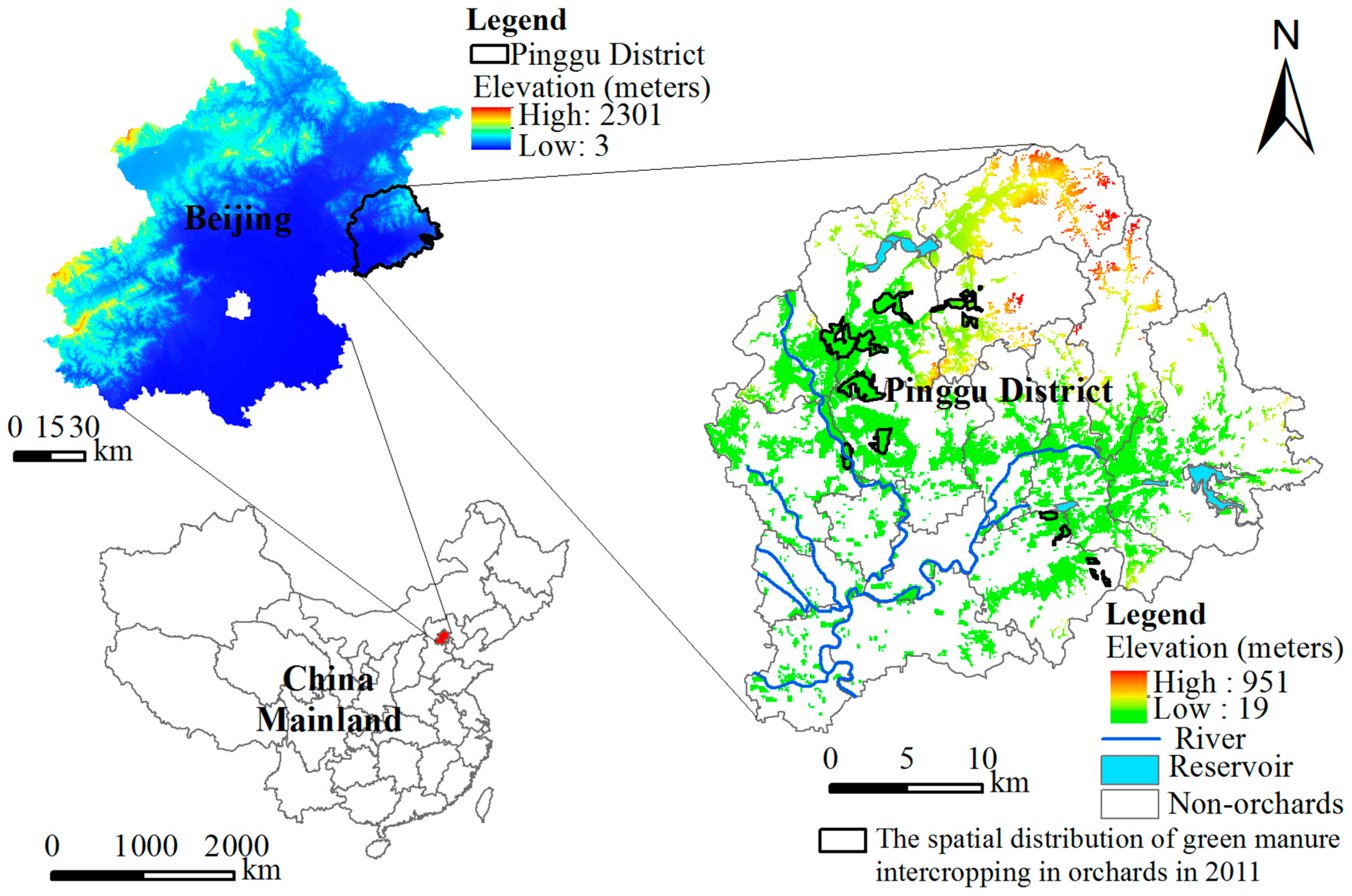
The Pinggu District (40°01′44″–40°22′39″N, 116°55′20″–117°24′09″E) is in the northeastern part of Beijing, China, and the terrain of the study area slopes from northeast to southeast. The elevations of the orchard patches are between 19 m and 951 m (Figure 1). The average annual rainfall is 542 mm. Mountainous terrain is dominant in the district. The warm temperate zone along the mountains stretches hundreds of miles, resulting in a sunny area with temperature fluctuations between day and night, which are quite suitable for fruit growth. Pinggu contains 16 towns and covers an area of 948.35 km², and orchards occupy almost 30% of this total area. The spatial distribution of orchards is shown in Figure 1. Fruit sales and crop production are major components of the local economy. In 2011, the local government began promoting green manure (Orychophragmus violaceus) intercropping in orchards, which currently cover a total area of 22,103 ha. The regions where green manure was promoted were mainly located in Dahuashan, Wangxinzhuang, and Xiongerzhai, which had a total combined orchard area of 1433 ha in 2011 (Figure 1).

2.2. Data and Processing

(1) The land-use map of the study area in 2011 was obtained from the Bureau of Land Resources in Beijing and was used to extract the spatial locations of the orchards in the study area; (2) the spatial distribution of orchards with intercropped green manure was obtained from the Beijing Soil and Fertilizer Station; (3) the data used for evaluating orchard productivity, including the active soil depth, soil texture, elevation, slope, aspect, available phosphorus content, available potassium content, organic matter content, guarantee of irrigation, and drainage capability, were obtained from the Beijing Digital Soil System; (4) the geophysical driving factors used in the CLUE-S model (i.e., the distributions of the nearest road, railway, river, lake, main town, and rural resident site) were obtained from the Beijing Digital Soil System. The shape index and connectivity of orchard patches were computed using the equations provided in Section 2.3.2; (5) socioeconomic factors, such as orchard areas, fruit yield, and agricultural practitioners, were obtained from the Statistical Yearbooks of the Pinggu District, Beijing (2012). All data were converted to the same projection with an equal grid size of 100 × 100 m.

2.3. Methods

2.3.1. Land Productivity Evaluation

Land productivity represents the comprehensive production capacity of orchards and is determined by the soil characteristics, natural conditions, and current management level. Assessment criteria usually proposed by experts and the Analytic Hierarchy Process(AHP)-based spatial multicriteria decision analysis (S-MCDA) method [50,51] were usually introduced to determine the criteria scores and weights [52,53,54,55,56,57].

In this paper, the assessment criteria and corresponding weights in land productivity evaluation are referred to the Rules for Cultivated Land Productivity Assessment in Beijing, China (DB11/T 1083-2014), published by Beijing Municipal Administration of Quality and Technology Supervision [58].

The evaluation process included four basic steps: dividing the evaluation units, building an evaluation indicators system, calculating the integrated orchard productivity index, and grading the productivity according to the evaluation scores.

(1) Evaluation units

In this paper, the graph overlay method was adopted to divide the evaluation units, which referred to the superposition of the land-use map and the corresponding soil map to obtain separate patches as evaluation units. The soil properties, landform, soil nutrient attributes, and soil management should be consistent in one assessment unit. Both qualitative and quantitative analyses were employed to analyze the land productivity in each evaluation unit. These data were uniformed with different scale. All data was processed by renowned experts, and the evaluation results were examined by a senior professional staff. Actually, we obtained the required data from the Beijing Digital Soil System directly.

(2) Indicators system

Four criteria levels, namely, the soil profile, site condition, soil nutrients, and soil management levels, were selected to assess orchard production, and 10 indicators were included (

Table 1. Indicators system for land productivity evaluation and quantification standards for each indicator.

Criteria Level	Index Level	Unit	Classification Standards of Indicators									Weight (%)
			100	80	70	60	40	30	20	10	-
Soil profile	Active soil depth	cm	≥100	100–80		80–60	60–30				<30 a	15.1
	Soil texture		Medium loam or heavy loam	Light loam		Sandy loam	Clay or sand				Gravelly soil b	22.8
Site condition	Elevation	m	<100	100–200		200–300	300–400		≥400			8.3
	Slope	°	<3 c	3–5		5–8	8–15		15–25		≥25 d	4.3
	Aspect	°	135–225		90–135 or 225–270		45–90 or 270–315			315–360 or 0–45		6.7
Soil nutrients	Available phosphorus content	mg kg−1	≥40	40–30		30–20	20–10		<10			3.2
	Available potassium content	mg kg−1	≥180	180–120		120–100	100–80		<80			3.8
	Organic matter content	g kg−1	≥30	30–20		20–15	15–10				<10	10.2
Soil management	Guarantee of irrigation		Fully satisfied		Basically satisfied		Generally satisfied			Without irrigation		21.3
	Drainage capability		High		Medium			Low				4.3

Note: ^a,b,d: if the active soil was <30 cm deep, the soil texture was gravelly, or the slope was >25°, the score for the evaluation unit was assigned as 10. ^c When the slope of the unit was <3°, the score of the aspect was assigned as 100.

). The weights of all evaluation indicators are referred to the Rules for Cultivated Land Productivity Assessment in Beijing, China (DB11/T 1083-2014) [58].

(3) Calculation of the integrated orchard productivity index (IPI)

The additive method was used to compute the IPI of each unit using the following equation:

$$IPI={\displaystyle \sum _{i=1}^{10}(F_i\times C_i)}$$

(1)

where IPI is the integrated index, F_i is the score of the evaluation factor of i, and C_i is the weight of the evaluation factor of i.

(4) Grades classification

The productivity was graded according to the distribution of the IPI via the frequency curve method. The grades classification can be observed in

Table 2. The grades of the IPI.

IPI	Grades
≥84	highest
75–84	higher
65–75	medium
53–65	lower
<53	lowest

.

2.3.2. Simulation of the Spatial Distribution of Green Manures Based on the CLUE-S Model

The CLUE-S model is a grid-based model, which features the transformation of all types related to green manure intercropping and spatial allocation with two distinct modules: non-spatial and spatial modules.

(1) Classification of the types of the base year

Similar to the land-use classification type of the CLUE-S model, the following five types related to green manure planting were classified: orchards intercropped with green manure (M1), lower orchard productivity without intercropping with green manure (M2) (note: the lowest class only accounted for 0.52% of the total orchards and consequently could not meet the requirement that the number of each category should be greater than 1% to allow the CLUE-S model to run smoothly. Thus, the lowest and lower classes were merged to meet this requirement), medium orchard productivity without intercropping with green manure (M3), higher orchard productivity without intercropping with green manure (M4), and the highest orchard productivity without intercropping with green manure (M5). In the future, it will be possible to shift the M2, M3, M4, and M5 systems to M1 because the demand for green manure application is increasing. The specific transformation is obtained from the characteristics under different scenarios.

(2) Non-spatial module

This module was used to calculate the demands of the five modes in two scenarios in 2020. The assumption was that we would promote the same areas of green manure under the two scenarios.

Scenario 1: Based on the local agriculture development program, the local government aims to promote the incorporation of green manure in orchards at the rate of 1500 ha per year. In this case, the total area of M1 orchards would increase by 1500 ha each year. According to the characteristics of the orchards, priority is given to orchards with relatively low productivity (M2); thus, the total area of M2 orchards will decrease by 1500 ha each year. When the demand of M2 decreases to 0, the demand of M3 begins to decrease. When the demand of M3 decreases to 0, the demand of M4 decreases, and so forth. However, the demands in the non-spatial module cannot be assigned as 0 according to the requirement of the CLUE-S model; thus, we used 1 ha instead of 0 to guarantee that the model could run smoothly.

Scenario 2: The total area of the M1 orchards increases by 1500 ha per year. Priority is given to the orchards with very high productivity (M5), which would decrease by 1500 ha each year. When the areas of M5 decrease to 0, we can decrease the demand of M4, and so forth. We also used 1 ha instead of 0 to guarantee that the model would run smoothly.

(3) Spatial module

The spatial module can receive all types of demands from the non-spatial module and can control the spatial locations of the five types by using the regression coefficient of the driving factors and the probability distribution over the parameters. The selection of driving factors is shown in

Table 3. Selection of driving factors.

Classification of Driving Factors	Driving Factors	Unit
Location condition	Distance to the nearest road (X1)	m
	Distance to the nearest railway (X2)	m
	Distance to the nearest river (X3)	m
	Distance to the nearest lake (X4)	m
Land use condition	Distance to the nearest main town (X5)	m
	Distance to the nearest rural resident site (X6)	m
Spatial characteristics of patches	Shape index (X7)	-
	Connectivity of orchard patches (X8)	-
Socioeconomic condition	Orchard areas (X9)	ha
	Fruit yield (X10)	t
	Agricultural practitioners (X11)	person

.

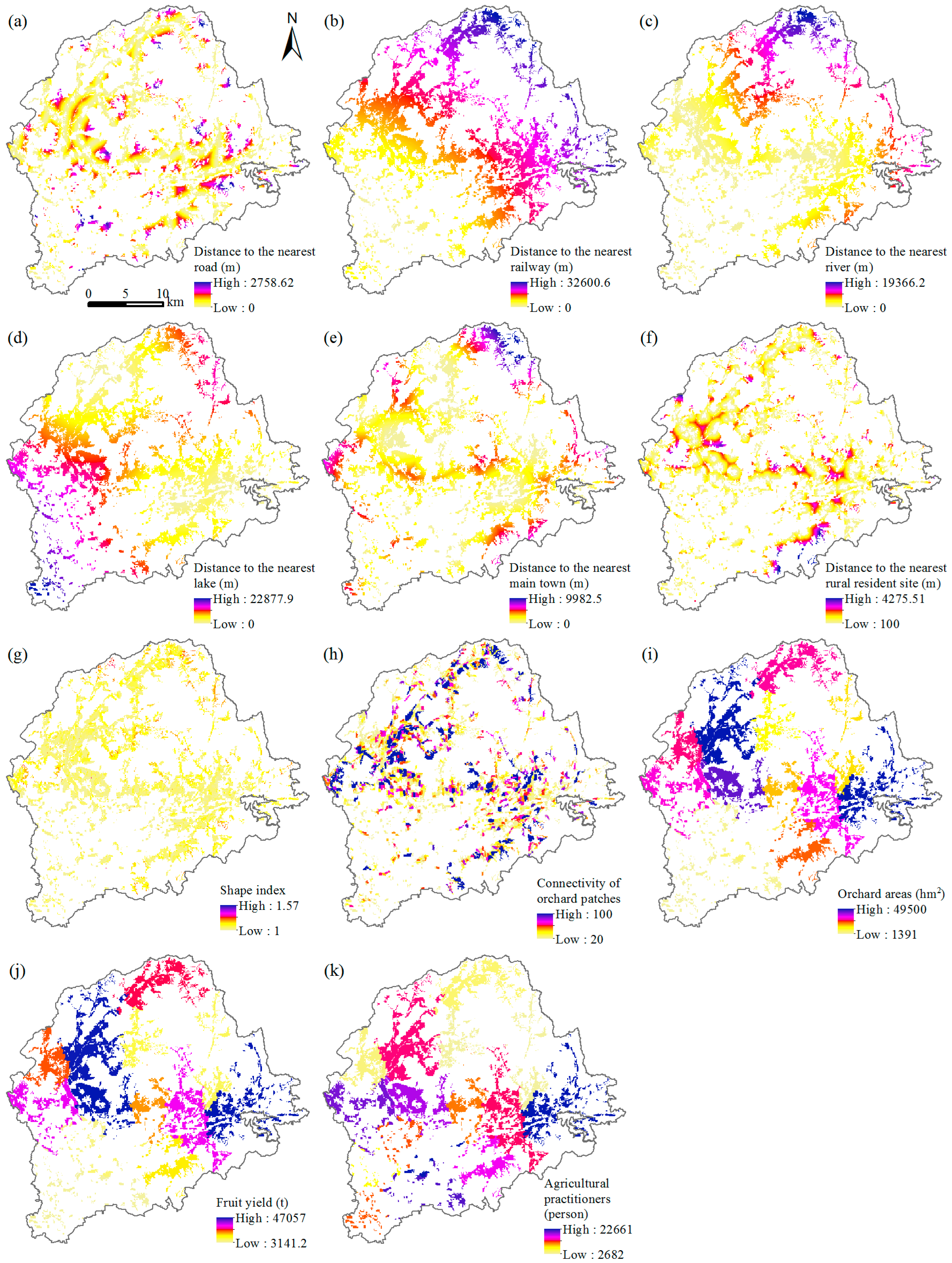
Specifically, X₁, X₂, X₃, and X₄ were used to describe the transport accessibility. X₅ and X₆ represented the distance to the main town (farms’ market inside) and the far and near conditions for orchard management by agricultural practitioners. All the distances (X₁ to X₆) could be calculated via the Euclidean distance by using ArcGIS 10.1. Furthermore, the orchards with regular shape and high connectivity were prioritized. X₇ was measured using the fractal dimension index (FRAC) from landscape ecology, which is shown in Equation (2) [59]. X₈ was gauged by Equation (3) [60]. X₉, X₁₀, and X₁₁ were the key socioeconomic variables impacting the green manure promotion.

$$FRAC=\frac{2\log (p/4)}{\log (a)}$$

(2)

where p and a are the perimeter and area of the patch, measured in m and m², respectively. The range of the index varies from 1 to 2 (without units). Higher values correspond to more complicated shapes.

$$Q=\{\begin{array}{l}20a\ge 5.23{\mathrm{hm}}^2\\ 20+80\times \frac{a-5.23}{20.94-5.23}5.23{\mathrm{hm}}^2<a\le 20.94{\mathrm{hm}}^2\\ 100a>20.94{\mathrm{hm}}^2\end{array}$$

(3)

where Q is the connectivity of the patch and ranges from 20 to 100 (without units) and a is the area of the patch measured in m². Higher values indicate a higher degree of connectivity among the patches.

The regression coefficients and the probabilities of the transformation of the spatial allocation features were defined using the following logit model:

$$\ln (\frac{P_i}{1-P_i})={\beta }_0+{\beta }_1{X}_{1,}{}_i+{\beta }_2{X}_{2,i}+\dots +{\beta }_n{X}_{n,i}$$

(4)

where P_i is the probability of the grid i containing a particular mode, and X_n,i is the driving variable. The coefficient (β) is estimated using logit regression, in which the actual spatial distribution of a certain mode acts as the dependent variable, with the value of i ranging from 1 to 5 for M1 to M5.

The conversion settings are composed of two parameters, the conversion elasticity (ELAS) and the transition matrix. The first parameter, ranging from 0 (easy conversion) to 1 (irreversible conversion), was determined via expert knowledge. In this paper, the ELAS values were 1, 0.8, 0.6, 0.4, and 1, 0.4, 0.6, 0.8 for scenarios 1 and 2, respectively. The second parameter has values of 0 (irreversible transition) or 1 (easy conversion) and indicates what conversions are possible for each mode. In this study, M1 could not be converted to other types. The conversion matrix can be observed in

Table 4. Conversion matrix for the five types of the two scenarios.

	M1	M2	M3	M4	M5
M1	1	0	0	0	0
M2	1	1	1	1	1
M3	1	1	1	1	1
M4	1	1	1	1	1
M5	1	1	1	1	1

Note: In the matrix, 0 indicates an easy conversion and 1 indicates an irreversible conversion. The lines inside the matrix indicate conversion-out, and the columns indicate switching-in.

.

The transformation between different modes will determine what changes occur. For each grid cell i, the total probability ($TPRO{P}_{i,u}$) was estimated for each mode by using the following equation:

$$TPRO{P}_{i,u}=P_{i,u}+ELA{S}_u+ITE{R}_u$$

(5)

where $TPRO{P}_{i,u}$ is the suitability of grid i for type u, $ELA{S}_u$ is the conversion parameter for type u, and $ITE{R}_u$ is an iteration variable that is specific to mode u and indicates the relative competitive strength of mode u.

3. Results

3.1. Land Productivity Evaluation Results

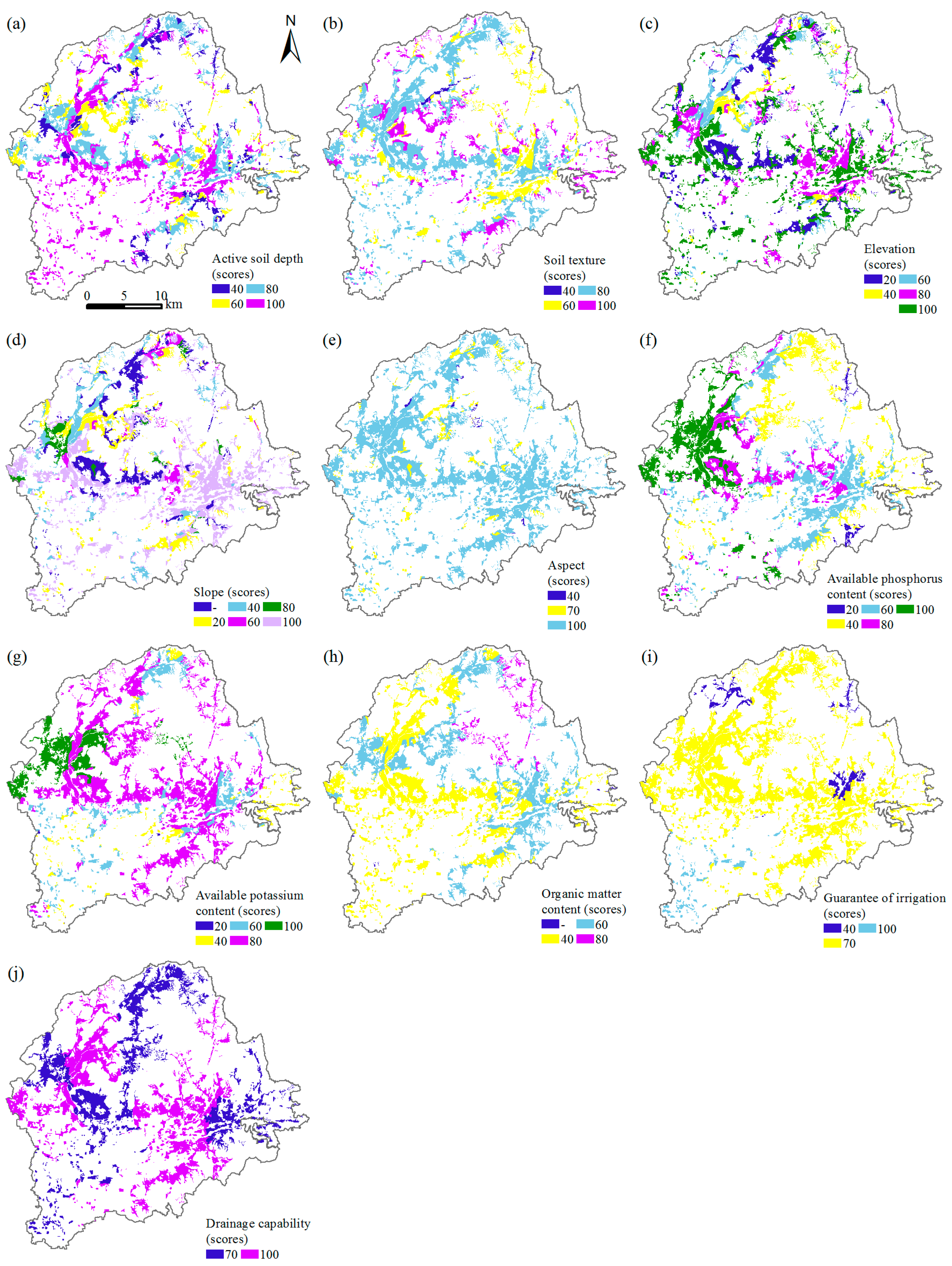
By overlaying the land-use map and the corresponding soil map, 5239 evaluation units were assigned. The scores of all evaluation units for the assessment indicators can be seen in Figure 2.

Patches with high scores of active soil depth still had high rankings of slope and drainage capability. The same situation occurred in the indicators of available potassium content and available phosphorus content. Also, no orchard patches had an active soil depth thinner than 30 cm. Also, sandy loam and light loam occupied large percentages, and there was no gravelly soil texture. In addition, the topography sloped from northeast to southeast. The aspect of the assessment units was mainly between 135 to 225 degrees, so most of the units achieved a score of 100 for this indicator. No units were detected with a slope higher than 25 degrees in the study area. For the soil nutrients properties, a very small percentage of patches had an organic matter content lower than 10 g kg⁻¹. Many of the units had an organic matter content of 10–15 g kg⁻¹ or 15–20 g kg⁻¹. Regarding the guarantee of irrigation, most of the units were second-grade, namely, “basically satisfied”. Patches without irrigations were not found.

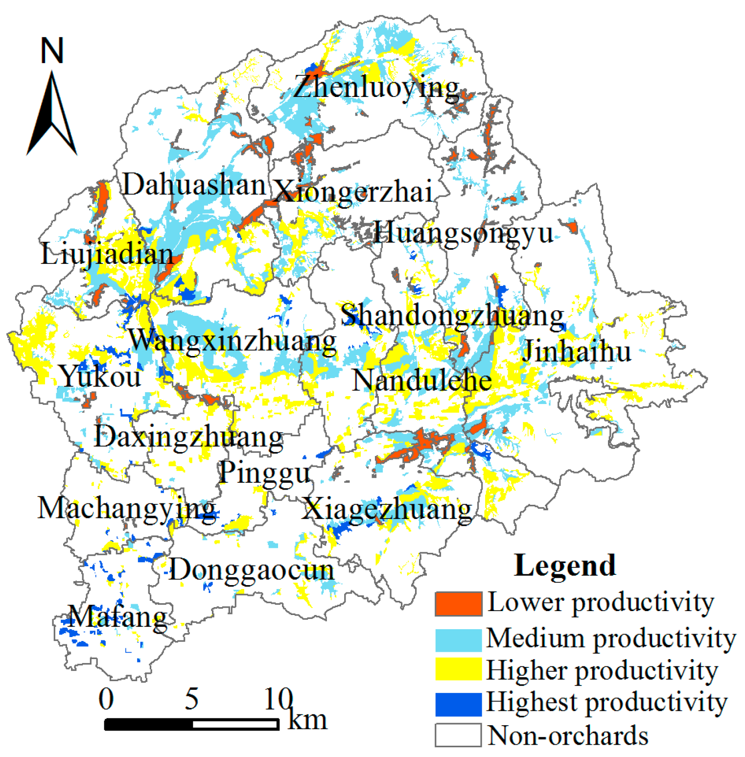
The final IPIs were estimated using Equation (1), and the land productivity was originally divided into the following categories: lowest, lower, medium, higher, and highest. Since the lowest and lower classes were merged to meet this requirement (reasons could be found in Section 2.3.2), the land productivity was graded into four categories: lower, medium, higher, and highest classes. The spatially explicit results are shown in Figure 3. The four grades accounted for 10.48%, 37.62%, 45.71%, and 6.19%, respectively, of the entire orchard study area.

3.2. Spatial Distribution of All Categories of 2011

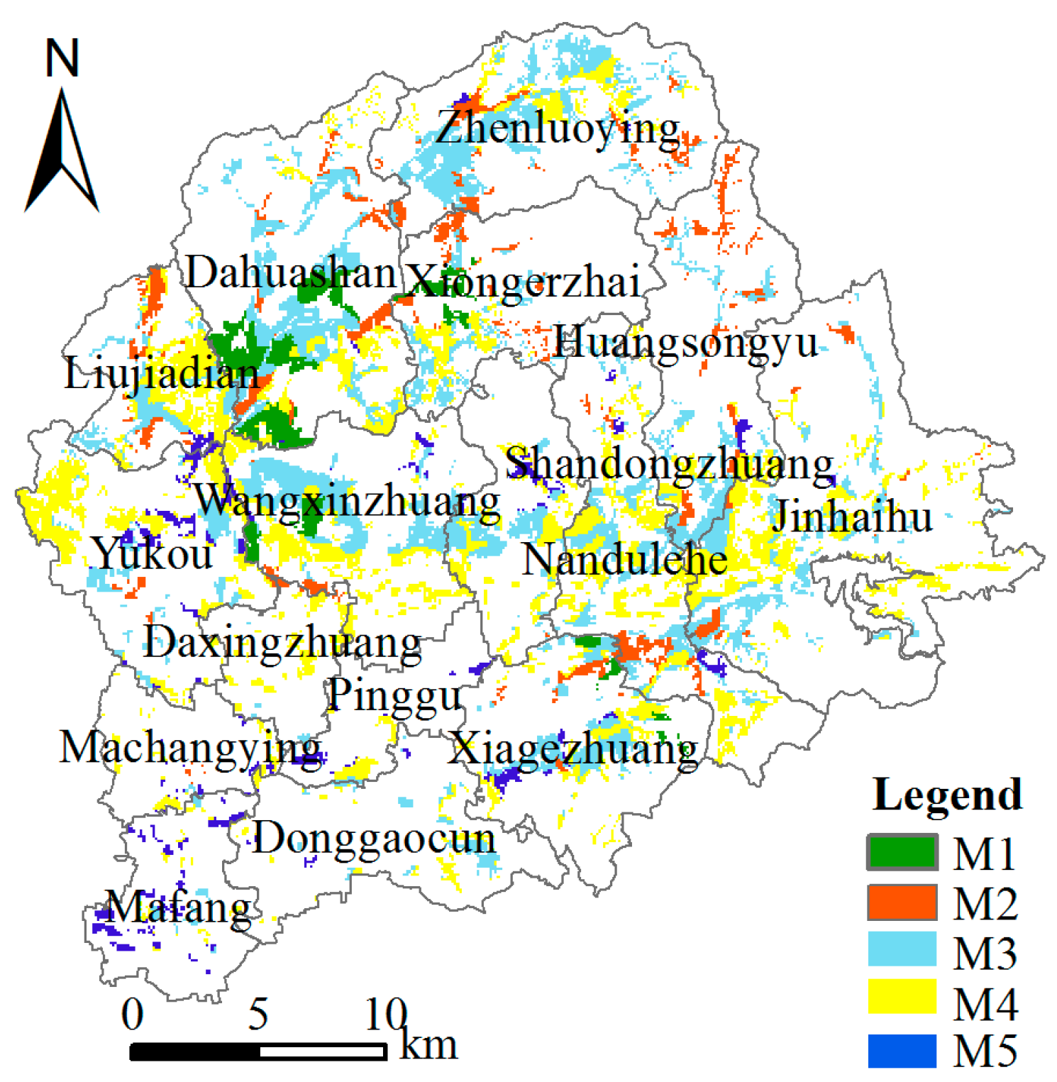
The spatial distribution of all categories was obtained by overlaying the spatial distribution of green manure intercropping in orchards in 2011 (shown in Figure 1) with Figure 3. The spatial distributions of all types can be found in Figure 4. M1 was mainly located in Dahuashan, Wangxinzhuang, and Xiongerzhai, which had a total combined orchard area of 1393 ha in 2011. M2 was scattered in the townships of Dahuashan, Zhenluoying, Huangsongyu, and Nandulehe. In addition, M3 was mainly located in the northern and central townships in the study region, i.e., southern Dahuashan, central Zhenluoying, and the middle of Wangxinzhuang. M4 was located in southern Yukou, eastern Liujiadian, central and southern Nandulehe, and western Jinhaihu, and M5 was distributed sporadically in the orchards of all the townships, but with very small percentages.

3.3. Regression Analysis of Categories Changes

A logistic regression model was used to explore the relationship between the classified categories and the related driving forces. To estimate the coefficients (β’s) of the logit model, a logistic regression procedure was used with the actual land-use pattern as a dependent variable. A statistical package, i.e., the SPSS, was used to regress land use upon its explanatory factors. A stepwise regression procedure was used to select the relevant factors from a larger set of location characteristics.

Figure 5 shows the maps of the driving forces in the study region.

Table 5. Logit regression results for the different types in the study area.

Driving Factors	M1		M2		M3		M4		M5
	ß	Exp(ß)	ß	Exp(ß)	ß	Exp(ß)	ß	Exp(ß)	ß	Exp(ß)
Constant	8.5464	5148.1876	−2.2717	0.1031	1.6665	5.2936	−3.9650	0.0190	−9.5359	0.0001
X1	−0.0373	0.9634	−0.0426	0.9583	0.0387	1.0395	−0.0170	0.9831
X2	−0.0520	0.9493	0.0085	1.0085	0.0063	1.0063	0.0017	1.0017	0.0098	1.0098
X3	0.0357	1.0363	0.0030	1.0030	−0.0088	0.9912	−0.0112	0.9889	−0.0241	0.9762
X4	−0.0327	0.9678	−0.0156	0.9845	0.0081	1.0081	0.0017	1.0017	0.0220	1.0222
X5	−0.0195	0.9807	0.0528	1.0542	−1.9093	0.1482	0.0089	1.0089	−0.0155	0.9846
X6	0.0699	1.0724	−0.8731	0.4177	0.0977	1.1026	−0.0291	0.9713
X7	−4.8340	0.0080	−0.0095	0.9905	−0.0055	0.9945	3.1032	22.2691	4.0341	56.4900
X8	0.0127	1.0128	−0.0426	0.9583	0.0049	1.0049	−0.2468	0.7813	0.5924	1.8083
X9	0.0104	1.0105	0.0085	1.0085	−0.0012	0.9988	0.0020	1.0020
X10	0.0040	1.0040	0.0030	1.0030	0.0387	1.0395	−0.0025	0.9975	−0.0051	0.9949
X11	−0.0003	0.9997	−0.0156	0.9845	0.0063	1.0063	0.0061	1.0061	0.0108	1.0109
ROC	0.850		0.848		0.863		0.897		0.896

presents these driving forces and their coefficients for the logistic regression. The results showed that different categories had different driving forces that contributed to their locations. The logit regression results were further examined by using receiver operating characteristic (ROC) indices. We could see that the shape index (X₇) had the highest regression coefficient in Table 5. The orchards with regular shape were prioritized for promoting green manure.

3.4. Quantitative Analysis of the Five Types under the Two Scenarios

The demands for all types were calculated according to the situational characteristics presented in Section 2.3.2 and are shown in

Table 6. Requirements of the five types of the different scenarios in 2020 (ha).

Years	Scenario 1					Scenario 2
	M1	M2	M3	M4	M5	M1	M2	M3	M4	M5
2011	1393	2167	8749	8622	1172	1393	2167	8749	8622	1172
2012	2893	667	8749	8622	1172	2893	2167	8749	8293	1
2013	4393	1	7915	8622	1172	4393	2167	8749	6793	1
2014	5893	1	6415	8622	1172	5893	2167	8749	5293	1
2015	7393	1	4915	8622	1172	7393	2167	8749	3793	1
2016	8893	1	3415	8622	1172	8893	2167	8749	2293	1
2017	10,393	1	1915	8622	1172	10,393	2167	8749	793	1
2018	11,893	1	415	8622	1172	11,893	2167	8041	1	1
2019	13,393	1	1	7536	1172	13,393	2167	6541	1	1
2020	14,893	1	1	6036	1172	14,893	2167	5041	1	1

. Also, we compared the simulated numbers with the requirements and the relative error between them (

Table 7. The precision of the simulation and validation results of the CLUE-S model.

Types	Demand (ha)		Simulated Results (ha)		Relative Error (%)
	Scenario 1	Scenario 2	Scenario 1	Scenario 2	Scenario 1	Scenario 2
M1	14,893	14,893	14,888	14,889	−0.03	−0.03
M2	1	2167	1	2176	0	0.42
M3	1	5041	1	5036	0	−0.10
M4	6036	1	6030	1	−0.10	0
M5	1172	1	1183	1	0.94	0

), which was very small and suggested that the CLUE-S model could correctly conform to the demands.

3.5. Spatial Expansion of Green Manure Intercropping in 2020

The simulated spatial locations of all types via CLUE-S under the two scenarios for 2020 are shown in Figure 6.

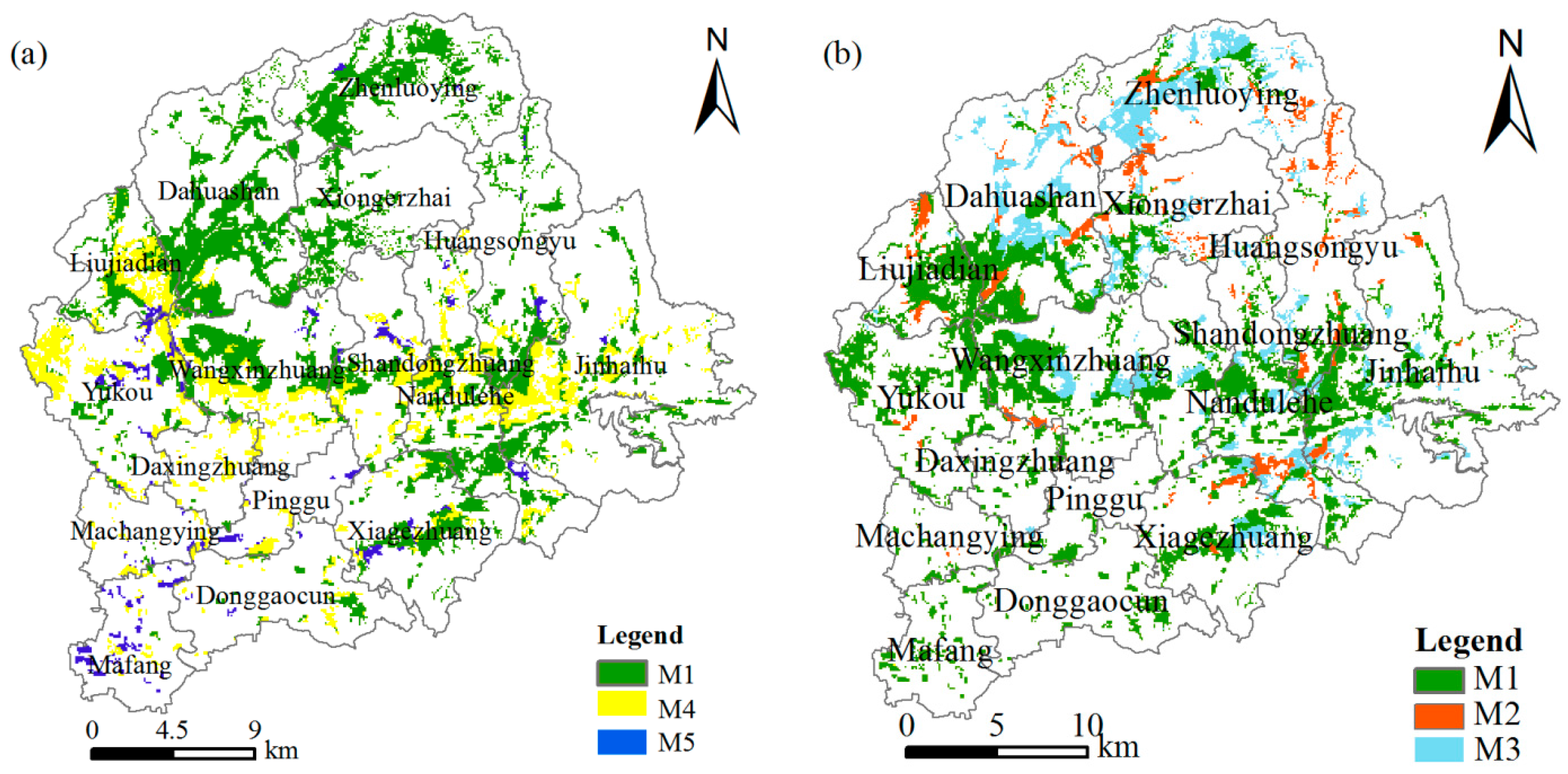
In Figure 6a, the spatial distribution of M2 and M3 decreased rapidly and disappeared; thus, the M2 and M3 orchards were all converted to M1 orchards, and only three modes, i.e., M1, M4, and M5, remained. M1 primarily appeared in Zhenluoying and in the northern regions of Dahuashan and Huangsongyu. M1 were mainly located in the middle of the study region, e.g., south of Dahuashan, west of Xiongerzhai, in southern Liujiadian, west of Wangxinzhuang, in the center of Shandongzhuang, and south and in the middle of Nandulehe. M1 also occurred in very scattered patches in the southern regions of the study area, i.e., Xiagezhuang, Machangying, and Donggaocun.

In Figure 6b, the M4 and M5 disappeared in the simulation, which meant that these types of orchards were shifted to M1 and that only three modes, i.e., M1, M2, and M3, remained. The promotion of green manure in orchards mainly occurred in the middle of the study area, such as in southern Dahuashan, western Xiongerzhai, eastern Liujiadian, northern Yukou, western Wangxinzhuang, the middle of Shandongzhuang, central Nandulehe, and western Jinhaihu. M1 covered a smaller area in the northern regions of Dahuashan and Zhenluoying. In addition, the M1 orchards appeared in some very scattered patches in the southern regions of the study area, i.e., Daxingzhuang, Pinggu, Xiagezhuang, Donggaocun, and Mafang.

3.6. The Accuracy of the Simulation of the CLUE-S Model

The CLUE-S model was originally applied in the field of simulating land-use changes and has rarely been used in other research areas. In this study, the CLUE-S model was introduced to simulate the spatial distribution of orchards with green manure according to different land-use type conversions and spatial allocations. Two key aspects must be considered to verify the accuracy of the CLUE-S model, i.e., the ROC coefficient and the Kappa index. The ROC coefficient is used to test the effectiveness of the logistic regression. A ROC greater than 0.7 suggests a strong ability to illustrate the correlation between the modes and the driving variables [61]. In this study, the respective ROCs for M1 through M5 were 0.850, 0.848, 0.863, 0.897, and 0.896, thus all greater than 0.7, which suggests that the selected driving factors explained well the spatial changes of the five types. The other index, which is used to evaluate the feasibility of the model for simulating the whole modes, is the Kappa index [62], which should be at least 0.85. The simulated map of 2013 was compared with the actual map via ENVI 4.8, and the Kappa index was 0.90, which indicated it could capture the future trend of green manure in developing orchards. The high Kappa index potentially resulted from the very short time interval (3 years only), the very small changes in the driving variables, and the conversion setting from 2011 to 2013. A long-term simulation should be tested in future research.

4. Discussion

4.1. Land Productivity Evaluation

In this paper, land productivity evaluation was incorporated in the simulation of the spatial location of green manure. The categories classification of the base year regarding intercropping green manure or non-intercropping, largely depends on the orchard productivity assessment results. Elevation, soil properties, and social-economic factors (i.e., guarantee of irrigation and drainage capability) can affect the productivity results. We referred to the Rules for Cultivated Land Productivity Assessment in Beijing, China (DB11/T 1083-2014) [58] to determine the assessment criteria and weights. Soil profile, site condition, soil nutrients, and soil management factors were included in the indicators system. However, the dynamics of land productivity evaluation were not considered because of the unavailability of data. Since the incorporation of green manure in the orchard can improve soil productivity [38], the soil quality should be monitored and kept updated annually, thus providing a guidance for annual green manure management [63].

4.2. Mechanisms of Spatial Changes of Green Manure under Different Scenarios

Different spatially explicit results were processed under two scenarios. In general, the outcomes showed the driving factors that affect green manure expansion at the grid scale, whereas the implementing strategies directly determined the spatial arrangement of green manuring at a regional scale.

In Figure 6, under scenario 1, the promotion of green manure was prioritized for relatively lower- and medium-productivity orchards. The spatial distribution of M1 in scenario 1 was more concentrated than in scenario 2. Some townships, such as Pinggu and Mafang, did not include any M1. Approximately 30% of the orchards for which green manure application was promoted had high productivity. These orchards were located in north of Zhenluoying and Dahuashan and south of Xiongerzhai and Xiagezhuang because continuous orchard patches and socioeconomic factors with high values occurred in this area. Because the orchards with lower (M2), medium (M3), and higher productivity (M4) already meet the demands for promoting green manure in 2020, the orchards with highest productivity should not be introduced to green manure. As shown in Table 7, green manure was introduced to only 11 ha of orchards with the highest productivity, which resulted in a small relative error (only 0.94%).

For scenario 2, green manure development was preferred in the highest- and relatively higher-productivity orchards. In addition, approximately 42% of the orchards with medium land productivity, primarily located in south of Dahuashan, Wangxinzhuang, Shandongzhuang, and Nandulehe and in the central region of Jinhaihu, were chosen for green manure planting. The result was due to the flat terrain, higher soil attributes, and convenient traffic conditions. Because the orchards with the highest (M5) and higher (M4) productivity and some of the orchards with medium productivity (M3) already met the demands for promoting green manure in 2020, green manure should not be promoted for orchards with the lowest productivity. As shown in Table 7, only the 9 ha orchards with very low fertility introduced green manure. This result was caused by the error of the model, with a relative error of only 0.42%.

4.3. Implications for Orchard Green Manure Management

Due to the deterioration of soil and environment, the traditional organic green manure has gained great attention again. Green food without overuse of chemical fertilizers or heavy metals is required. Promoting green manure is thought to be one effective way to relieve the current usage of high amounts of chemicals. To establish a sustainable intercropping system, a stable and suitable application of green manure is urgently required. For green manure which is in the phase of recovery and development, it is a key point to grasp the future spatial potential to promote this crop. The methods showed in this study can guide in mapping the potential of promoting green manure in space and in visually establishing a future trend for developing green manure in orchards.

As shown in Figure 6, the spatial distribution of M1 in scenario 1 was more concentrated than in scenario 2. This means that if people prioritize the lower-productivity orchard to develop green manure intercropping (scenario 1), they can focus on a concentrated area and conduct the green manuring intensively. This strategy can lead to a decreased labor time and a decreased labor cost. Alternatively, if people prioritize orchard with higher productivity to promote green manure intercropping (scenario 2), green manure can be extended to most of the study area. This strategy enables more farmers and villages to benefit from the expansion of green manure. The different strategies should be balanced according to their characteristics.

In addition, socioeconomic factors can have an effect on green manure planting. Future research is needed to incorporate policy into the simulation because the promotion of green manure is somewhat affected by policy makers. As shown in this study, the shape index of orchard patches dominated among the selected driving factors. Regular shaped patches were prioritized for promoting green manure. The contributions of the driving factors should be tested further in order to analyze the spatial pattern under different scenarios [64].

5. Conclusions

To scientifically and accurately simulate the spatial distribution of green manure interplanted in orchards, the evaluation of orchard productivity and the CLUE-S model were incorporated in this study. Similar to the land-use type classification, five types of land productivity for planting green manure were classified, which acted as source data for running the simulation. Two scenarios were proposed to describe two promotion strategies. The good ROC and Kappa indices revealed the strong ability of the model to map the spatially explicit distribution of the research object. Because of the different scenario characteristics, the transformation of M1 occurred distinctively in space. The spatial location of M1 in scenario 1 was more concentrated than in scenario 2.

In conclusion, the simulated outcomes could achieve our goals and revealed that selected driving variables have an effect on green manure expansion at a grid scale, whereas the different implementing strategies directly determine the spatial arrangement of green manuring at a regional scale. The evaluation of ecological indicators and the simulation of future spatial patterns of green manuring are essential for informing an extensive use and management of green manure.

In future research, a range of scenarios should be developed to determine the optimal scenarios, and a sustainable planning for the recovery of green manure is urgently needed [65]. In addition, the dynamics of land productivity evaluation should be included in a long-time simulation. Apart from intercropping green manure, it should also be determined how to capture the trend of the rotating green manure in space. Research that combines the simulation model and an ecological model may provide a more integrated view for promoting green manure in China and guide the formulation of a sound policy for developing green manure.

References

- Robertson, G.P.; Paul, E.A.; Harwood, R.R. Greenhouse Gases in Intensive Agriculture: Contributions of Individual Gases to the Radiative Forcing of the Atmosphere. Science 2000, 289, 1922–1925. [Google Scholar] [CrossRef] [PubMed]
- Tejada, M.; Gonzalez, J.L.; García-Martínez, A.M.; Parrado, J. Application of a green manure and green manure composted with beet vinasse on soil restoration: Effects on soil properties. Bioresour. Technol. 2008, 99, 4949–4957. [Google Scholar] [CrossRef] [PubMed]
- Tejada, M.; Gonzalez, J.L.; García-Martínez, A.M.; Parrado, J. Effects of different green manures on soil biological properties and maize yield. Bioresour. Technol. 2008, 99, 1758–1767. [Google Scholar] [CrossRef] [PubMed]
- Babulicová, M. Influence of fertilization on winter wheat in crop rotations and in long-term monoculture. Plant Soil Environ. 2008, 54, 190–196. [Google Scholar]
- Sharma, A.R.; Behera, U.K. Nitrogen contribution through Sesbania green manure and dual-purpose legumes in maize–wheat cropping system: Agronomic and economic considerations. Plant Soil 2009, 325, 289–304. [Google Scholar] [CrossRef]
- Miyazawa, K.; Murakami, T.; Takeda, M.; Murayama, T. Intercropping green manure crops—Effects on rooting patterns. Plant Soil 2009, 331, 231–239. [Google Scholar] [CrossRef]
- Hirel, B.; Tétu, T.; Lea, P.J.; Dubois, F. Improving Nitrogen Use Efficiency in Crops for Sustainable Agriculture. Sustainability 2011, 3, 1452–1485. [Google Scholar] [CrossRef]
- Liebman, M.; Graef, R.L.; Nettleton, D.; Cambardella, C.A. Use of legume green manures as nitrogen sources for corn production. Renew. Agric. Food Syst. 2012, 27, 180–191. [Google Scholar] [CrossRef]
- Talgre, L.; Lauringson, E.; Roostalu, H.; Astover, A.; Makke, A. Green manure as a nutrient source for succeeding crops. Plant Soil Environ. 2012, 58, 275–281. [Google Scholar]
- Kaur, J.; Singh, J.P. Long-term effects of continuous cropping and different nutrient management practices on the distribution of organic nitrogen in soil under rice-wheat system. Plant Soil Environ. 2014, 60, 63–68. [Google Scholar]
- Yang, Z.; Zheng, S.; Nie, J.; Liao, Y.; Xie, J. Effects of Long-Term Winter Planted Green Manure on Distribution and Storage of Organic Carbon and Nitrogen in Water-Stable Aggregates of Reddish Paddy Soil Under a Double-Rice Cropping System. J. Integr. Agric. 2014, 13, 1772–1781. [Google Scholar] [CrossRef]
- Chocano, C.; García, C.; González, D.; Melgares de Aguilar, J.; Hernández, T. Organic plum cultivation in the Mediterranean region: The medium-term effect of five different organic soil management practices on crop production and microbiological soil quality. Agric. Ecosyst. Environ. 2016, 221, 60–70. [Google Scholar] [CrossRef]
- Zhang, D.; Yao, P.; Zhao, N.; Yu, C.; Cao, W.; Gao, Y. Contribution of green manure legumes to nitrogen dynamics in traditional winter wheat cropping system in the Loess Plateau of China. Eur. J. Agron. 2016, 72, 47–55. [Google Scholar] [CrossRef]
- Mancinelli, R.; Marinari, S.; Di Felice, V.; Savin, M.C.; Campiglia, E. Soil property, CO2 emission and aridity index as agroecological indicators to assess the mineralization of cover crop green manure in a Mediterranean environment. Ecol. Indic. 2013, 34, 31–40. [Google Scholar] [CrossRef]
- Bossuyt, H.; Denef, K.; Six, J.; Frey, S.D.; Merckx, R.; Paustian, K. Influence of microbial populations and residue quality on aggregate stability. Appl. Soil Ecol. 2001, 16, 195–208. [Google Scholar] [CrossRef]
- Denef, K.; Six, J.; Bossuyt, H.; Frey, S.D.; Elliott, E.T.; Merckx, R.; Paustian, K. Influence of dry–wet cycles on the interrelationship between aggregate, particulate organic matter, and microbial community dynamics. Soil Biol. Biochem. 2001, 33, 1599–1611. [Google Scholar] [CrossRef]
- Denef, K.; Six, J.; Paustian, K.; Merckx, R. Importance of macroaggregate dynamics in controlling soil carbon stabilization: Short-term effects of physical disturbance induced by dry–wet cycles. Soil Biol. Biochem. 2001, 33, 2145–2153. [Google Scholar] [CrossRef]
- Six, J.; Bossuyt, H.; Degryze, S.; Denef, K. A history of research on the link between (micro)aggregates, soil biota, and soil organic matter dynamics. Soil Tillage Res. 2004, 79, 7–31. [Google Scholar] [CrossRef]
- Harrison-Kirk, T.; Beare, M.H.; Meenken, E.D.; Condron, L.M. Soil organic matter and texture affect responses to dry/wet cycles: Effects on carbon dioxide and nitrous oxide emissions. Soil Biol. Biochem. 2013, 57, 43–55. [Google Scholar] [CrossRef]
- Harrison-Kirk, T.; Beare, M.H.; Meenken, E.D.; Condron, L.M. Soil organic matter and texture affect responses to dry/wet cycles: Changes in soil organic matter fractions and relationships with C and N mineralisation. Soil Biol. Biochem. 2014, 74, 50–60. [Google Scholar] [CrossRef]
- Porqueddu, C.; Re, G.A.; Sanna, F.; Piluzza, G.; Sulas, L.; Franca, A.; Bullitta, S. Exploitation of Annual and Perennial Herbaceous Species for the Rehabilitation of a Sand Quarry in a Mediterranean Environment. Land Degrad. Dev. 2016, 27, 346–356. [Google Scholar] [CrossRef]
- Foucault, Y.; Lévêque, T.; Xiong, T.; Schreck, E.; Austruy, A.; Shahid, M.; Dumat, C. Green manure plants for remediation of soils polluted by metals and metalloids: Ecotoxicity and human bioavailability assessment. Chemosphere 2013, 93, 1430–1435. [Google Scholar] [CrossRef] [PubMed]
- Frøseth, R.B.; Bakken, A.K.; Bleken, M.A.; Riley, H.; Pommeresche, R.; Thorup-Kristensen, K.; Hansen, S. Effects of green manure herbage management and its digestate from biogas production on barley yield, N recovery, soil structure and earthworm populations. Eur. J. Agron. 2014, 52, 90–102. [Google Scholar] [CrossRef]
- Piotrowska, A.; Wilczewski, E. Effects of catch crops cultivated for green manure and mineral nitrogen fertilization on soil enzyme activities and chemical properties. Geoderma 2012, 189–190, 72–80. [Google Scholar] [CrossRef]
- Zotarelli, L.; Zatorre, N.P.; Boddey, R.M.; Urquiaga, S.; Jantalia, C.P.; Franchini, J.C.; Alves, B.J.R. Influence of no-tillage and frequency of a green manure legume in crop rotations for balancing N outputs and preserving soil organic C stocks. Field Crops Res. 2012, 132, 185–195. [Google Scholar] [CrossRef]
- Zhang, D.; Yao, P.; Na, Z.; Cao, W.; Zhang, S.; Li, Y.; Gao, Y. Soil Water Balance and Water Use Efficiency of Dryland Wheat in Different Precipitation Years in Response to Green Manure Approach. Sci. Rep. 2016, 6, 26856. [Google Scholar] [CrossRef] [PubMed]
- Jiang, Y.; Kang, M.; Schmidt-Vogt, D.; Schrestha, R.P. Identification of agricultural factors for improving sustainable land resource management in northern Thailand: A case study in Chiang Mai Province. Int. J. Sustain. Dev. World Ecol. 2007, 14, 382–390. [Google Scholar] [CrossRef]
- Wei, J.; Xiao, D.; Zeng, H. Sustainable development of an agricultural system under ecological restoration based on Emergy analysis: A case study in northeastern China. Int. J. Sustain. Dev. World Ecol. 2008, 15, 103–112. [Google Scholar] [CrossRef]
- Kourouxou, M.; Siardos, G.; Iakovidou, O.; Kalburtji, K. Organic farmers in islands: Agricultural management and attitude towards the environment. Int. J. Sustain. Dev. World Ecol. 2008, 15, 553–564. [Google Scholar] [CrossRef]
- Tesio, F.; Ferrero, A. Allelopathy, a chance for sustainable weed management. Int. J. Sustain. Dev. World Ecol. 2010, 17, 377–389. [Google Scholar] [CrossRef]
- Gao, J.; Cao, W.; Li, D.; Xu, M.; Zeng, X.; Me, J.; Zhang, W. Effects of long-term double-rice and green manure rotation on rice yield and soil organic matter in paddy field. Acta Ecol. Sin. 2011, 31, 4542–4548. [Google Scholar]
- Lan, Y.; Huang, G.; Yang, B.; Chen, H.; Wang, S. Effect of green manure rotation on soil fertility and organic carbon pool. Trans. Chin. Soc. Agric. Eng. 2014, 30, 146–152. [Google Scholar]
- Verburg, P.H.; Eickhout, B.; van Meijl, H. A multi-scale, multi-model approach for analyzing the future dynamics of European land use. Ann. Reg. Sci. 2007, 42, 57–77. [Google Scholar] [CrossRef]
- Verburg, P.H.; Overmars, K.P. Combining top-down and bottom-up dynamics in land use modeling: Exploring the future of abandoned farmlands in Europe with the Dyna-CLUE model. Landsc. Ecol. 2009, 24, 1167–1181. [Google Scholar] [CrossRef]
- Verburg, P.H.; van de Steeg, J.; Veldkamp, A.; Willemen, L. From land cover change to land function dynamics: A major challenge to improve land characterization. J. Environ. Manag. 2009, 90, 1327–1335. [Google Scholar] [CrossRef] [PubMed]
- Britz, W.; Verburg, P.H.; Leip, A. Modelling of land cover and agricultural change in Europe: Combining the CLUE and CAPRI-Spat approaches. Agric. Ecosyst. Environ. 2011, 142, 40–50. [Google Scholar] [CrossRef]
- Verburg, P.H.; Soepboer, W.; Veldkamp, A.; Limpiada, R.; Espaldon, V.; Mastura, S.S.A. Modeling the Spatial Dynamics of Regional Land Use: The CLUE-S Model. Environ. Manag. 2014, 30, 391–405. [Google Scholar] [CrossRef] [PubMed]
- Xie, Z.; Tu, S.; Shah, F.; Xu, C.; Chen, J.; Han, D.; Liu, G.; Li, H.; Muhammad, I.; Cao, W. Substitution of fertilizer-N by green manure improves the sustainability of yield in double-rice cropping system in south China. Field Crops Res. 2016, 188, 142–149. [Google Scholar] [CrossRef]
- Alam, M.Z.; Lynch, D.H.; Sharifi, M.; Burton, D.L.; Hammermeister, A.M. The effect of green manure and organic amendments on potato yield, nitrogen uptake and soil mineral nitrogen. Biol. Agric. Hortic. 2016, 32, 221–236. [Google Scholar] [CrossRef]
- Berberoğlu, S.; Akın, A.; Clarke, K.C. Cellular automata modeling approaches to forecast urban growth for adana, Turkey: A comparative approach. Landsc. Urban Plan. 2016, 153, 11–27. [Google Scholar] [CrossRef]
- Luo, G.P.; Yin, C.Y.; Chen, X.; Xu, W.Q.; Lu, L. Combining system dynamic model and CLUE-S model to improve land use scenario analyses at regional scale: A case study of Sangong watershed in Xinjiang, China. Ecol. Complex. 2010, 7, 198–207. [Google Scholar] [CrossRef]
- Zhu, Z.Q.; Liu, L.M.; Chen, Z.T.; Zhang, J.L.; Verburg, P.H. Land-use change simulation and assessment of driving factors in the loess hilly region—A case study as Pengyang County. Environ. Monit. Assess. 2009, 164, 133–142. [Google Scholar] [CrossRef] [PubMed]
- Zhang, L.P.; Zhang, S.W.; Zhou, Z.M.; Hou, S.; Huang, Y.F.; Cao, W.D. Spatial distribution prediction and benefits assessment of green manure in the Pinggu District, Beijing, based on the CLUE-S model. J. Integr. Agric. 2016, 15, 465–474. [Google Scholar] [CrossRef]
- Zhang, L.P.; Zhang, S.W.; Huang, Y.J.; Cao, M.; Huang, Y.F.; Zhang, H.Y. Exploring an ecologically sustainable scheme for landscape restoration of abandoned mine land: Scenario-based simulation integrated linear programming and CLUE-S model. Int. J. Environ. Res. Public Health 2016, 13, 354. [Google Scholar] [CrossRef] [PubMed]
- Herrero, M.; Thornton, P.K.; Bernués, A.; Baltenweck, I.; Vervoort, J.; van de Steeg, J.; Makokha, S.; van Wijk, M.T.; Karanja, S.; Rufino, M.C.; et al. Exploring future changes in smallholder farming systems by linking socio-economic scenarios with regional and household models. Glob. Environ. Chang. 2014, 24, 165–182. [Google Scholar] [CrossRef]
- Waiyasusri, K.; Yumuang, S.; Chotpantarat, S. Monitoring and predicting land use changes in the Huai Thap Salao Watershed area, Uthaithani Province, Thailand, using the CLUE-s model. Environ. Earth Sci. 2016, 75, 1–16. [Google Scholar] [CrossRef]
- Shrestha, S.; Htut, A.Y. Land Use and Climate Change Impacts on the Hydrology of the Bago River Basin, Myanmar. Environ. Model. Assess. 2016, 1–15. [Google Scholar] [CrossRef]
- Trisurat, Y.; Eawpanich, P.; Kalliola, R. Integrating land use and climate change scenarios and models into assessment of forested watershed services in Southern Thailand. Environ. Res. 2016, 147, 611–620. [Google Scholar] [CrossRef] [PubMed]
- Jiang, W.; Chen, Z.; Lei, X.; He, B.; Jia, K.; Zhang, Y. Simulation of urban agglomeration ecosystem spatial distributions under different scenarios: A case study of the Changsha–Zhuzhou–Xiangtan urban agglomeration. Ecol. Eng. 2016, 88, 112–121. [Google Scholar] [CrossRef]
- Malczewski, J. GIS and Multicriteria Decision Analysis; John Wiley and Sons: New York, NY, USA, 1999. [Google Scholar]
- Malczewski, J. GIS based multicriteria decision analysis: A survey of the literature. Int. J. Geogr. Inf. Sci. 2006, 20, 703–726. [Google Scholar] [CrossRef]
- Antognelli, S.; Vizzari, M. Landscape liveability spatial assessment integrating ecosystem and urban services with their perceived importance by stakeholders. Ecol. Indic. 2017, 72, 703–725. [Google Scholar] [CrossRef]
- Figueira, J.; Greco, S.; Ehrgott, M. Multiple Criteria Decision Analysis: State of the Art Surveys, Multiple Criteria Decision Analysis State of the Art Surveys; Springer: Berlin/Heidelberg, Germany, 2005. [Google Scholar]
- Mendoza, G.A.; Martins, H. Multi-criteria decision analysis in natural resource management: A critical review of methods and new modelling paradigms. For. Ecol. Manag. 2006, 230, 1–22. [Google Scholar] [CrossRef]
- Modica, G.; Merlino, A.; Solano, F.; Mercurio, R. An index for the assessment of degraded Mediterranean forest ecosystems. For. Syst. 2015, 24, 1–13. [Google Scholar] [CrossRef]
- Vizzari, M.; Modica, G. Environmental effectiveness of swine sewage management: A multicriteria AHP-based model for a reliable quick assessment. Environ. Manag. 2013, 52, 1023–1039. [Google Scholar] [CrossRef] [PubMed]
- Saaty, T.L. The Analytic Hierarchy Process; McGraw-Hill Inc.: New York, NY, USA, 1980. [Google Scholar]
- Beijing Municipal Administration of Quality and Technology Supervision. The Rules for Cultivated Land Productivity Assessment in Beijing, China (DB11/T 1083-2014); Beijing Municipal Administration of Quality and Technology Supervision: Beijing, China, 2014.
- Zhang, Z.F.; Chen, B.M.; Guo, Z.S. Indicator system for evaluating arable land consolidation potential. China Land Sci. 2004, 18, 37–43. (In Chinese) [Google Scholar]
- Li, G; Wu, C.F.; Cao, S.A. Study on indicators system of selecting cultivated land into prime farmland. J. Agric. Mech. Res. 2006, 8, 46–48. (In Chinese) [Google Scholar]
- Pontius, R.G., Jr.; Schneider, L.C. Land-cover change model validation by an ROC method for the Ipswich watershed, Massachusetts, USA. Agric. Ecosyst. Environ. 2001, 85, 239–248. [Google Scholar] [CrossRef]
- Gobin, A.; Campling, P.; Feyen, J. Logistic modelling to derive agricultural land use determinants: A case study from southeastern Nigeria. Agric. Ecosyst. Environ. 2002, 89, 213–228. [Google Scholar] [CrossRef]
- Nawaz, A.; Farooq, M.; Lal, R.; Rehman, A.; Hussain, T.; Nadeem, A. Influence of Sesbania Brown Manuring and Rice Residue Mulch on Soil Health, Weeds and System Productivity of Conservation Rice–Wheat Systems. Land Degrad. Dev. 2017, 28, 1078–1090. [Google Scholar] [CrossRef]
- Teng, Q.; Hu, X.-F.; Cheng, C.; Luo, Z.; Luo, F.; Xue, Y.; Jiang, Y.; Mu, Z.; Liu, L.; Yang, M. Ecological effects of rice-duck integrated farming on soil fertility and weed and pest control. J. Soils Sediments 2016, 16, 2395–2407. [Google Scholar] [CrossRef]
- Srivastava, P.; Singh, R.; Tripathi, S.; Raghubanshi, A.S. An urgent need for sustainable thinking in agriculture—An Indian scenario. Ecol. Indic. 2016, 67, 611–622. [Google Scholar] [CrossRef]
Figure 1.
Site and elevation of orchards in the study area.
Figure 2.
Scores of assessment indicators of all evaluation units. (The “-”in (d) means that the slope is higher than 25 degrees, and the “-” in (h) means that the organic matter content is lower than 10 g kg−1, according to Table 1.)
Figure 3.
The evaluation results of land productivity in the study area.
Figure 4.
The spatial distributions of five productivity-incorporated types of intercropping or non-intercropping green manure in 2011. Orchards intercropped with green manure (M1); lower orchard productivity without intercropping with green manure (M2); medium orchard productivity without intercropping with green manure (M3); higher orchard productivity without intercropping with green manure (M4); highest orchard productivity without intercropping with green manure (M5).
Figure 5.
Maps of the driving factors in the study region.
Figure 6.
The spatial distribution map of the different planting models under two scenarios in 2020: (a) Scenario 1; (b) Scenario 2.