Evaluating Grid Size Suitability of Population Distribution Data via Improved ALV Method: A Case Study in Anhui Province, China


1
State Key Laboratory of Resources and Environmental Information System, Institute of Geographic Sciences and Natural Resources Research, Chinese Academy of Sciences, Chaoyang District, Beijing 100101, China
2
University of Chinese Academy of Sciences, Beijing 100049, China
3
CIGIS (CHINA) LIMITED, Beijing 100007, China
*
Author to whom correspondence should be addressed.
Sustainability 2018, 10(1), 41; https://doi.org/10.3390/su10010041
Submission received: 28 September 2017
/
Revised: 21 December 2017
/
Accepted: 22 December 2017
/
Published: 25 December 2017
(This article belongs to the Section Sustainable Urban and Rural Development)
Abstract
:Accurate grid size suitability evaluations are necessary to enhance the spatialization quality of gridded population distributions. This paper proposes an improved average local variance (ALV) method to express discrepancies in population density and was validated in Anhui Province, China. A dataset consisting of 14 spatial scales, from 100 m to 900 m, and 1000 m to 5000 m, was processed by both the proposed and traditional ALV methods. Line graphs of two sets of ALV values and grid sizes were comparatively analyzed to evaluate the grid size suitability. The ALV trends calculated by the proposed method encompassed more accurate and useful features compared to the traditional method. The case study results showed that the 200 m grid size accurately expresses the population distribution characteristics of Anhui Province. The standard deviation (SD) index was adopted to validate these results; the proposed ALV method was proven valuable both in theory and practice for assessing grid size suitability. The method may be further improved by determining the essential laws of ALV values based on grid characteristics, and by enhancing the adaptability to various locations.
1. Introduction
Population data spatialization is conducted to unearth implicit information from traditional statistical data and distribute it across the geo-grid [1], making it a fundamental precondition for integration among spatial datasets and for accurately simulating population spatial distribution laws [2,3]. The characteristics of population distribution patterns vary among different grid sizes [4]. The primary goal of spatialization is the selection of a suitable grid size [5] that reflects the desired population distribution characteristics. To this effect, grid size suitability must be accurately evaluated to improve spatialization quality.
Population distributions are scale-dependent [6]. Any suitable grid size is closely related to the regional features and the research purpose [7]. Many recent researchers have explored grid sizes of population spatial data based on specific regional features. Du G. et al. [6], for example, proved that population distribution depends on scale by applying geo-statistics methods to assess the spatial auto-correlation and variability of Shenyang City. Results were based on population distribution data with grains from 100 m to 1000 m. In addition, Ye, J. et al. [8] have found that grid size suitability varied from different kinds of data sources, using a mathematical statistics method based on population grid data and statistical data of Yiwu City, Zhejiang Province. Wang, P. et al. [9] used a spatial autocorrelation index to analyze the spatialization characteristics of population density in the Shiyang River Basin, showing that the range from 8000 m to 10,000 m comprised suitable grid sizes.
The local variance (LV) was first proposed by Woodcock and Strahler to investigate the spatial structure of images as the variance calculated for the pixel values. This was performed by passing an n × n moving window (3 × 3 window size was originally suggested [10]), then obtaining the mean of all local variance (Average Local Variance (ALV)) of the whole image as an indicator of the local variability of the image [10,11,12]. The spatial distributions of local features can also be obtained for further analysis. The semi-variance method can also be used to select appropriate image scale by calculating images’ semi-variance values through semivariogram [13,14,15]. When the semi-variance value is at its peak, the corresponding resolution can be selected as the most appropriate [13], in a similar way to the ALV method. Compared to ALV method, the semi-variance method involves more complex calculation, since some parameters need to be specified and iterative computation is necessary. This limits its practicability to some degree [16]. Based on this phenomenon, ALV method has been widely used in applications for selecting appropriate image resolutions [7], extracting Digital Elevation Model (DEM) characteristics [17], detecting spatial patterns in Remote Sensing(RS) images [18], optimizing image classifications [19], and evaluating image quality [20] among others. However, it has been rarely used to evaluate grid size suitability. Changes in moving window sizes cause variations in ALV values [11,16,21], which impact the spatial pattern detection process [18] and geomorphic characteristic extraction [22] of RS images to varying extents. In applying the ALV method, actual ground areas covered by the moving window vary due to the spatial resolutions of different images. ALV values of images computed based on variable factual ground area are not sufficiently comparable. The objectivity of any analysis based on ALV values is likewise insufficient [7]. The application range and effects of the ALV method, ultimately a useful tool for selecting appropriate spatial resolutions [10], merit further improvement.
This paper proposes an improved ALV method for the objective, comprehensive analysis of population data spatial distributions. The proposed method was tested in a case study using a set of gridded data produced from population statistical data and land use data at Anhui Province, China. The proposed method was further validated by comparing the traditional and improved ALV methods in regards to their analysis of grid size suitability. The objective of this study was to establish an improved ALV method that enhances the grid size rationality and spatialization quality of gridded population distributions. We hope that the results described in this paper may also provide a scientific basis for other manners of attribute statistical data spatialization techniques.
2. Materials and Methods
2.1. Study Area
Anhui Province, which is located in the hinterland of eastern China, extends from latitude 29°41′–34°38′ N and longitude 114°54′–119°37′ E. Anhui has been allocated to the urban cluster of the Yangtze River Delta, which is representative among both central and western regions. Anhui had a total population of 61.44 million in 2015 and contains 16 province-controlled cities, 6 county-level cities, and 56 counties covering a total area of 140,000 km2. Anhui Province has complicated terrain features encompassing Huaibei Plains, Jianghuai Hill, and Wannan Mountain, and the Yangtze and Huai rivers traverse the area from south to north. There is extreme disparity in the socio-economic development of southern and northern Anhui Province owing to historical and geographic factors [23]. This has a substantial effect on population spatial distribution characteristics across the region. These factors altogether made Anhui Province representative and practically substantial for the purposes of this study.
2.2. Gridded Population Distribution Data
The very foundation of grid size suitability research is multiple-size gridded population distribution data. The sources used to produce the gridded population distribution dataset used in this study are shown in Table 1.
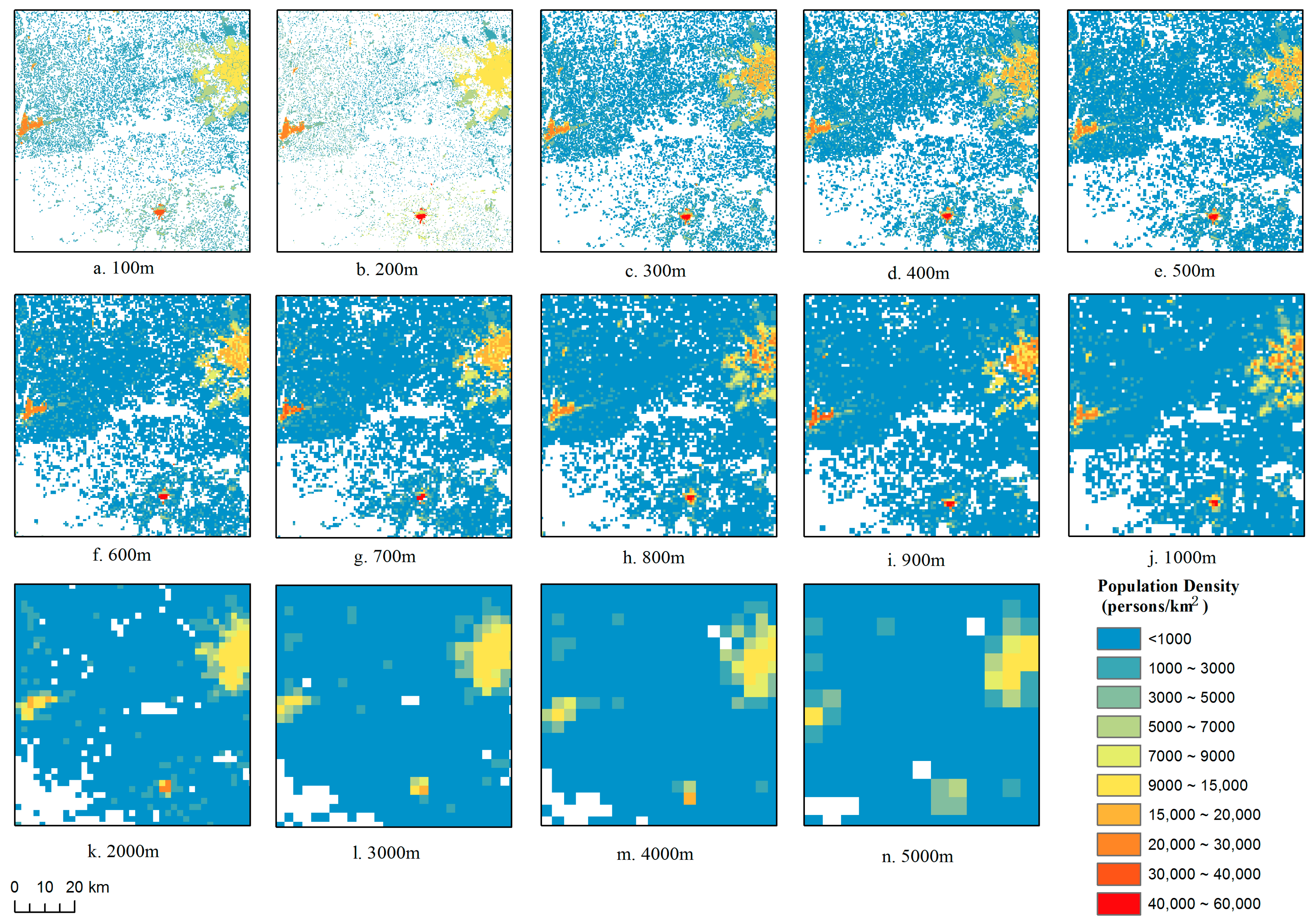
We adopted a multivariate statistics regression model to simulate population distribution patterns and to produce multiple-size gridded population distribution sets based on land use data. In the model, the independent variables included the areas of different land use types, and dependent variables were population statistical data [24]. We used the method first proposed by Yang, X. et al. [24] to process this data into 14 multiple-size gridded population distribution sets with ranges from 100 m to 900 m, and from 1000 m to 5000 m. Considering the readability, we chose four maps to display the changing trend of population distribution with the increasing of grid size, as shown in Figure 1. In all sizes of the gridded data, there is an area of accumulation at Hefei City, the provincial capital of Anhui. As grid size increases, different shades of blue indicating the population density become monotonic and blurred at the boundary.
2.3. Methods
2.3.1. ALV Method Application Principles
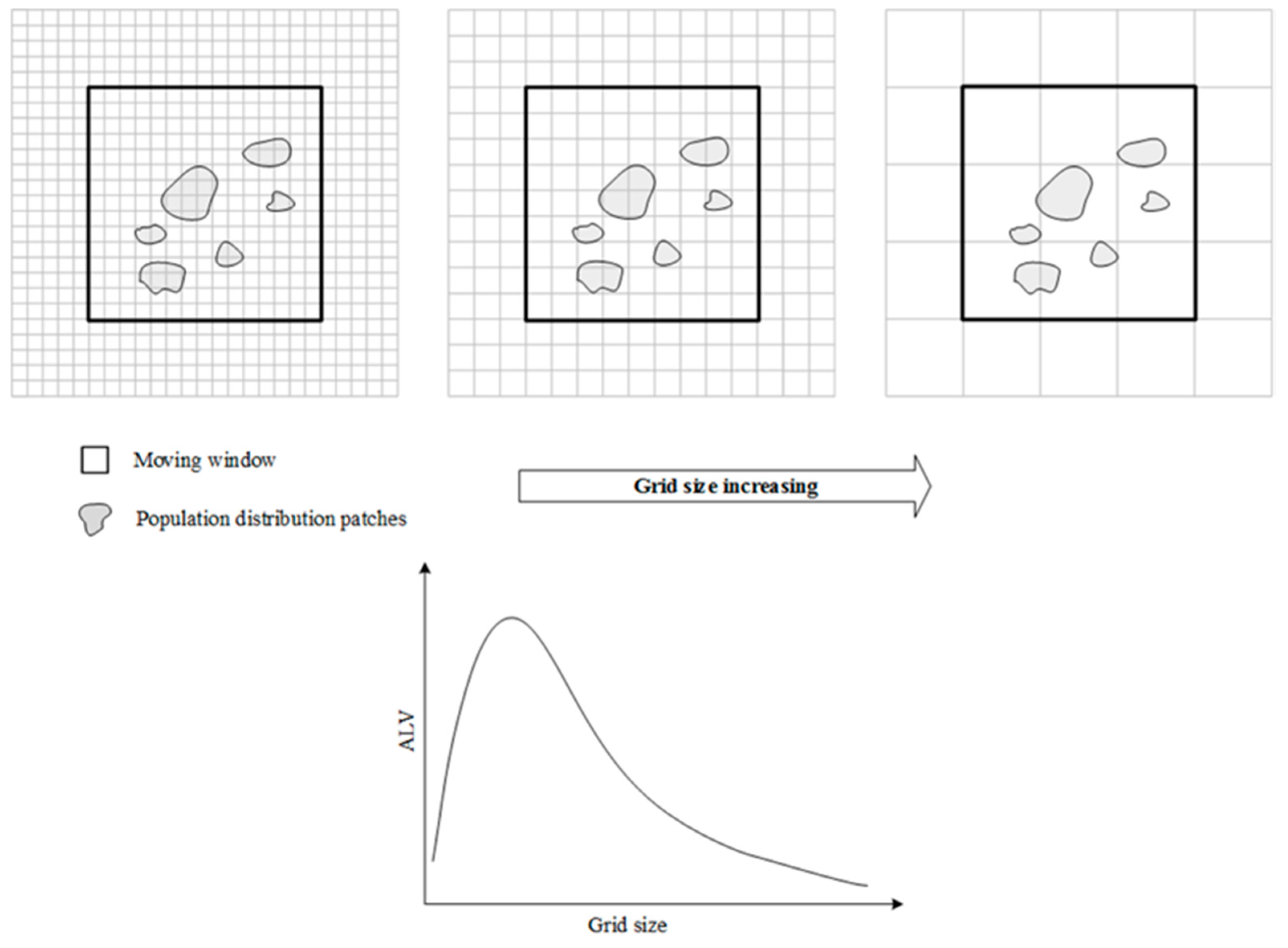
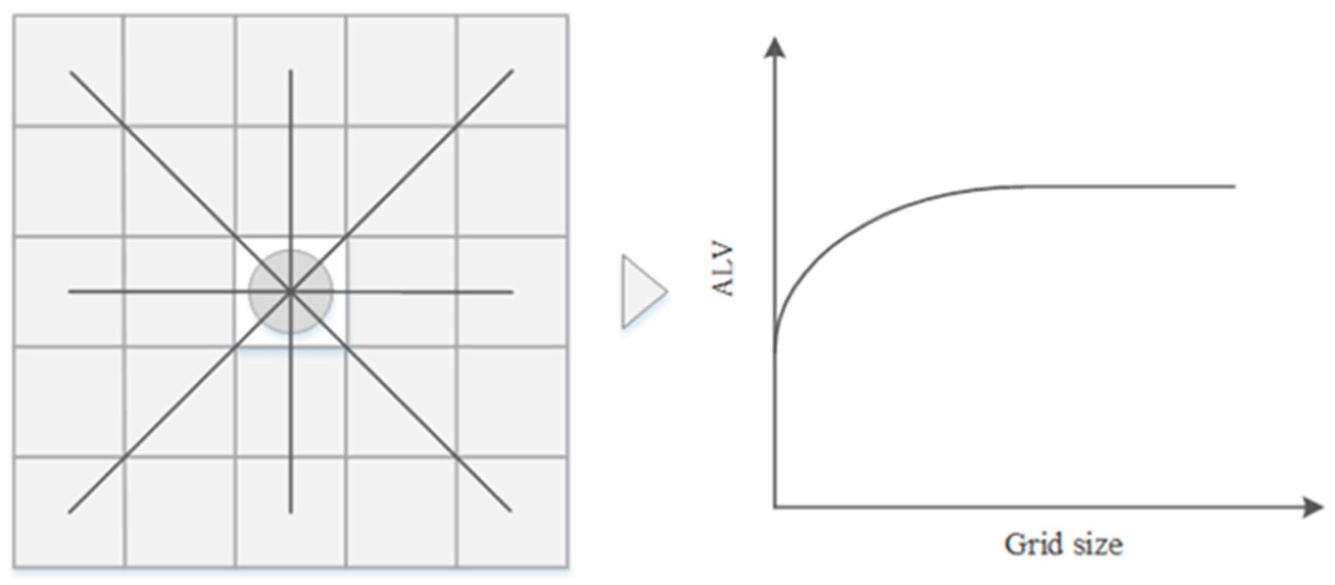
The theoretical basis of the ALV method is the spatial dependence theory, by which a greater distance between objects indicates a weaker spatial dependency between them [25]. ALV is used to evaluate grid size suitability by distinguishing differences between objects [26]. If the grid size is considerably finer than the objects in the image, much more cells will be highly correlated with their neighbors and the value of local variance will be low. If the objects approximate the grid size, then the likelihood of neighbors being similar decreases and the local variance rises. The local variance decreases as grid size increases and many different kinds of objects are contained in a single grid [10]. We used a moving c × c window to calculate the ALV value of the whole gridded data in this study, then analyzed the line graph of ALV value and grid size to evaluate grid size suitability [27].
The basic principles of applying the ALV method are illustrated in Figure 2 [19,27,28]. When the grid size is small enough, some adjacent grid cells belonging to the same class express the same population distribution patch. Their spatial dependence is stronger and the ALV value is lower, which indicates that this grid size does not display population density patches clearly and instead expresses different classifications. When the grid size increases, adjacent grid cells do express the different classifications of population density patches. As a result, their spatial dependence is weaker and the ALV value is higher. As grid size continually increases, one grid may cover more and different kinds of population density patches, whilst adjacent grid cells’ attributes become similar. Their spatial dependence becomes stronger and the ALV value decreases, suggesting that the grid size in question does not display population density patches clearly but does express different classifications. Generally speaking, when the ALV value peaks, the corresponding grid size can be considered as the best-suited value to expressing spatial distribution discrepancies in the study area [27]. The ALV value can be calculated as follows [27]:
where refers to the local variance of the grid cell (i, j); n is the total number of grid cells covered by the c × c moving window (c = 3, 5, 9, 15, 25 in this study); is the population density of the mth grid cell within the moving window; is the average population density of the grid cells within the c × c moving window. ALV is the average local variance of the study area on different grid sizes k (k = 100, 200, …, 900, 1000, …, 5000 m); N is the total number of the grid cells in the whole image.
2.3.2. Proposed ALV Method
The moving windows we plugged into the ALV method, as shown in Figure 2, have the same number of rows and columns. As grid size changes, then, the actual ground area covered by the moving windows differs. The “ground area” covered by moving window here just means “the plane area”, which was beneficial to calculating, comparing, and analyzing ALV values. Table 2 displays the actual ground area change trends corresponding to multiple grid sizes.
A series of ALV values of multiple-size gridded population distribution data, when calculated by the traditional ALV method based on moving windows covering different ground areas, cannot be analyzed objectively. The improvements we propose to ALV application are based on this phenomenon. ALV values can be controlled for comparativeness and objectiveness by ensuring the calculation windows cover the same actual ground areas in each set of population distribution data containing the same ground objects. To this effect, the actual ground areas of multiple-size gridded population distribution datasets are kept the same by adjusting the number of rows and columns in the moving windows. We increased the number of rows and columns when calculating smaller grid size data, and decreased them when calculating larger grid size data. Figure 3 [7,11,21] illustrates this theory.
Similar to the application of the traditional ALV method, when the size of gridded population distribution data is appropriate for distinguishing different classifications of population density patches, the ALV value in the proposed method peaks. At this point, the grid size in question is best-suited to expressing the spatial distribution of population density of the study area.
In executing the proposed ALV method, there is no guarantee that all the actual ground areas covered by moving windows of different gridded population distribution datasets are absolutely equal. There are some restrictions on the selection of moving windows, namely, the number of rows and columns must be odd. We tried to standardize the actual ground area by adjusting the number of rows and columns in the moving windows as described above—we simultaneously adopted a series of different ground areas to perform comparative analyses both horizontally and vertically. We tested ground areas of 225 km2, 625 km2, 2025 km2, 5625 km2, and 15,625 km2 and gave the gridded population distribution data the largest grid size (5000 m) with a series of moving windows: 3 × 3, 5 × 5, 9 × 9, 15 × 15, 25 × 25. The number of rows and columns of other gridded population distribution dataset’s moving windows were adjusted based on the 5000 m grid size window selection restrictions mentioned above.
Row and column quantities were selected under several important restrictions. The geographic characteristics of Anhui Province were taken into account, primarily to reflect the distances from south to north and from east to west of about 570 km and 450 km, respectively, and a total area of about 140,000 km2. We also ensured that the resulting window sizes were easy to calculate. Under these restrictions, the smallest ground area (225 km2) corresponds to a 3 × 3 window of 5000 m grid size data; the largest ground area (15,625 km2) exceeds 1/10 of total area (140,000 km2), which is large enough without weakening the different classification features to the point of a nonsensical calculation. Table 3 shows the theoretical and actual window sizes corresponding to theoretical and actual ground areas, as well as the area errors of different grid sizes.
3. Results
3.1. Results Based on Traditional ALV Method
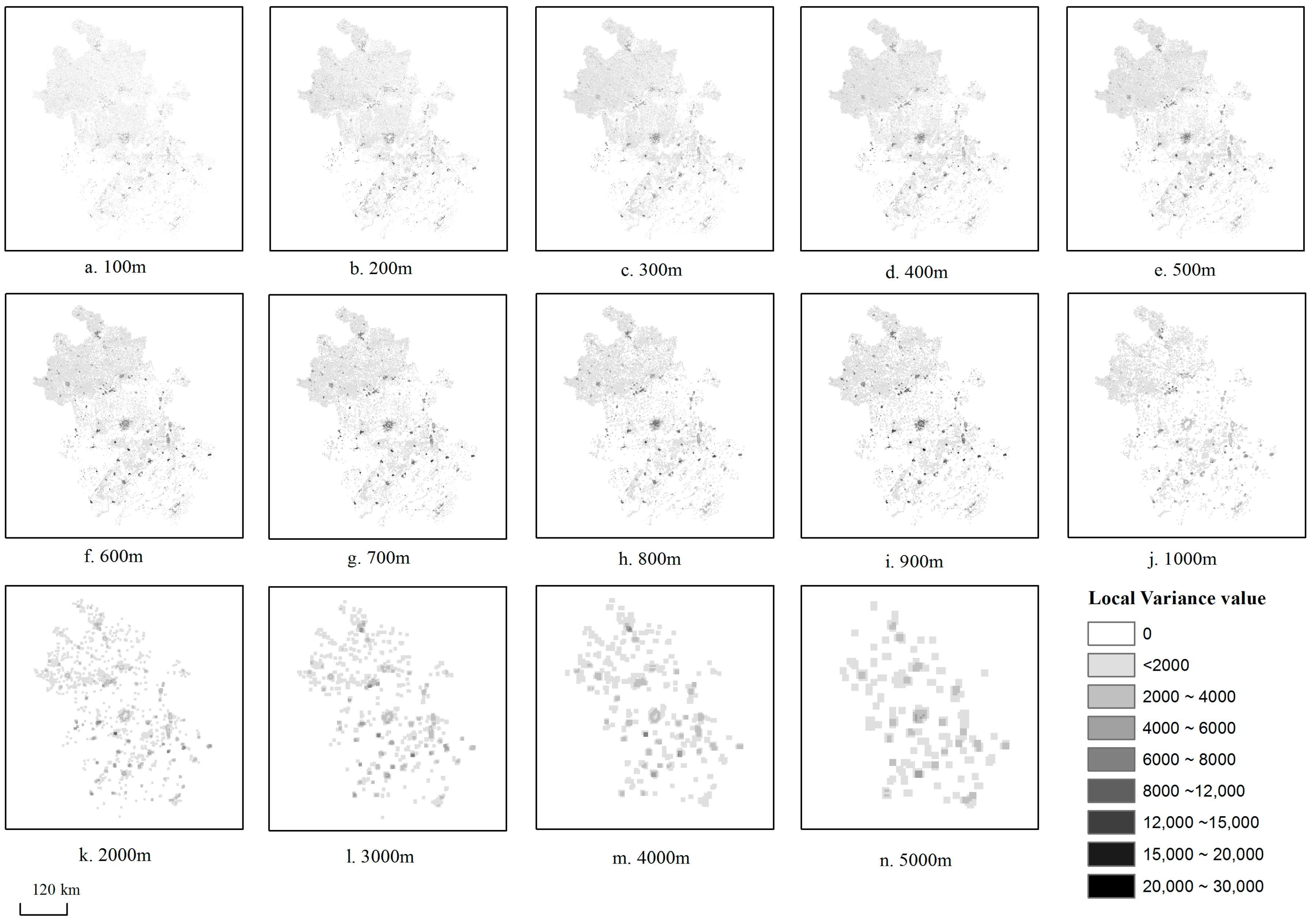
We used MATLAB R2015b to produce a series of local variance data based on multiple gridded population distribution data via the traditional ALV method, namely by keeping the moving windows’ number of rows and columns constant while the corresponding actual ground areas changed. Figure 4 displays the local variance data based on a 3 × 3 moving window. Several high-value areas are especially obvious over Hefei City under the relatively smaller grid sizes such as 200 m–900 m. The values of local average data under the other grid sizes are distributed relatively evenly.
Then, we used the “Spatial Analyst tool” of ArcGIS 10.1 to calculate the ALV value of each image. We drew line graphs showing different grid sizes on the x-axis and the calculated ALV values on the y-axis. Figure 5 shows the variations in ALV values under the 14 grid sizes calculated by the traditional ALV method. When comparing the ALV values vertically, under the same grid size, increasing window sizes caused the ALV values to increase. When comparing the ALV values horizontally (namely, different grid sizes with the same window size), the values increased sharply from 100 m to 200 m and dropped from 200 m to 300 m. From 300 m to 800 m, the values fluctuated. They increased substantially from 800 m to 900 m, then decreased sharply from 900 m to 1000 m, then increased again from 1000 m to 5000 m. We identified two obvious peaks among all the values corresponding to grid sizes of 200 m and 900 m. The changes in ALV values were altogether inconsistent among the five different window sizes.
3.2. Results Based on Proposed ALV Method
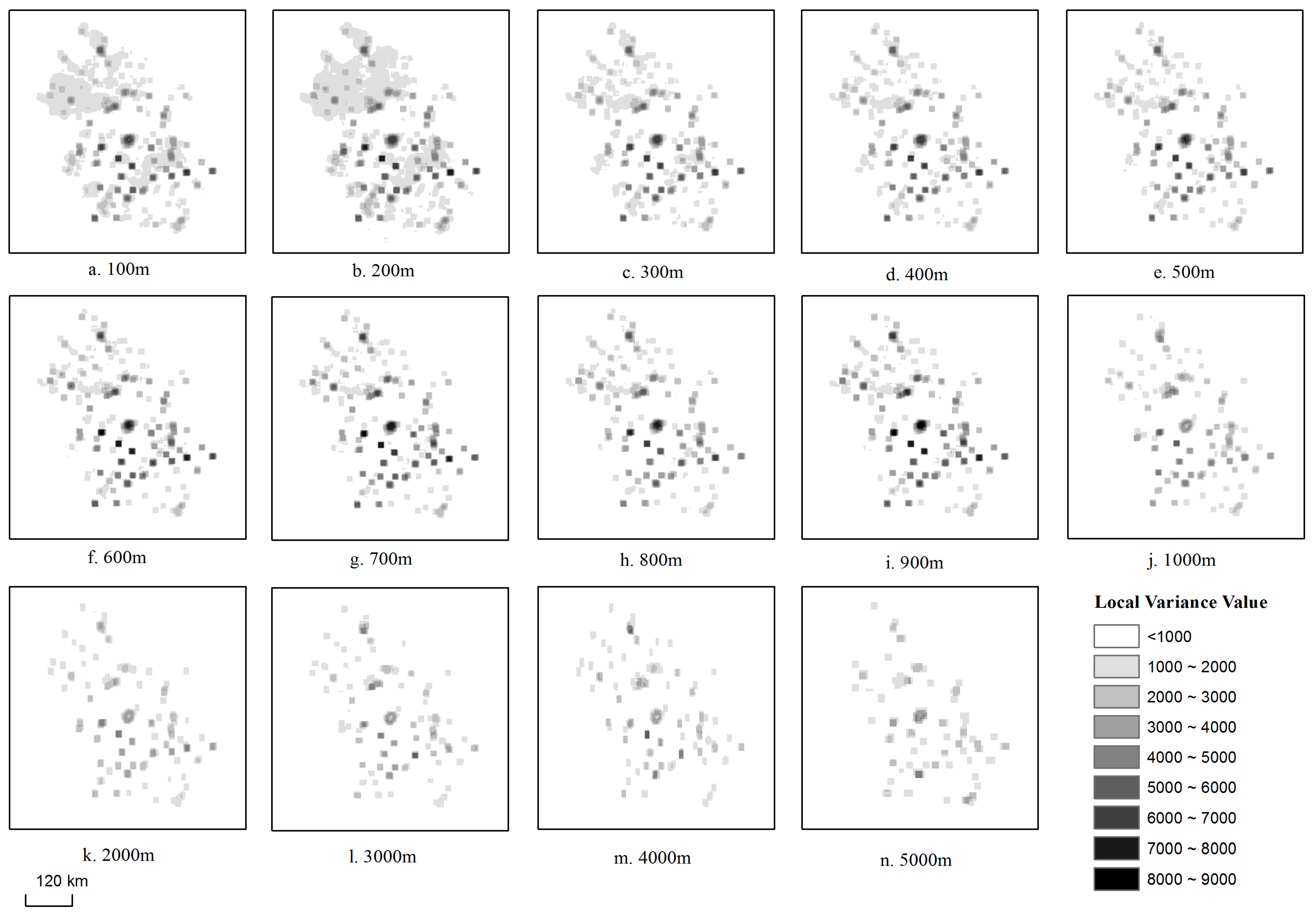
We next used MATLAB R2015b to produce a series of local variance data based on multiple gridded population distribution data via the proposed ALV method, namely where the moving windows’ number of rows and columns are adjusted to maintain the corresponding actual ground areas. Figure 6 shows the local variance data based on 225 km2 ground area. There are some high-value areas under the relatively smaller grid size from 100 m to 900 m. The colors indicate where local variance values decrease as grid size increases.
Then, we used the “Spatial Analyst tool” of ArcGIS 10.1 to calculate the ALV value of each image. We again drew line graphs showing different grid sizes on the x-axis and the calculated ALV values on the y-axis. Figure 7 shows the variations in ALV values across the 14 grid sizes calculated by the proposed ALV method. The ALV values increase as ground area increased regardless of grid size when compared vertically. Compared horizontally, there were some interesting differences among the ALV values with different grid sizes. From 100 m to 200 m, the values increased dramatically. From 200 m to 300 m, they quickly decreased. From 300 m to 800 m, the values fluctuated, but to a lesser extent than the results shown in Figure 5. The values increased substantially from 800 m to 900 m, then decreased sharply from 900 m to 1000 m and further from 1000 m to 5000 m. On the whole, there was only one key peak value corresponding to grid size of 200 m, which was different to the traditional ALV where the highest value is different for different window sizes. There was a secondary peak under the 900 m grid size, but it was not substantial compared to the key peak value. The ALV values appeared to be coherent and express consistent trends across the five different actual ground areas we tested.
4. Discussion
4.1. Comparative Analysis
We found that a larger moving window size or actual ground area created higher ALV values regardless of the grid size of the gridded population distribution data (Figure 5 and Figure 7), as calculated by both the traditional and proposed ALV method. As shown in Figure 8 [12], for any one piece of spatial data, a larger moving window covered more ground object classifications, resulting in higher local variance and ALV values. When the moving window was large enough to cover all the ground objects, the local variance actually represented the variance of the whole dataset. The ALV value did not increase with the moving window in this case.
Under the proposed method, each of the five series of ALV values have only the one peak value, which is easily observed corresponding to a grid size of 200 m (Figure 7). This was not the case for the traditional ALV method, which was affected by the moving window size. For example, the peak value based on the 3 × 3 moving window corresponded to the 200 m grid size, while the peak value based on the 25 × 25 moving window corresponded to the 900 m grid size. The ALV values obtained by a calculation window covering the same actual ground area were more objective and comparable than those obtained via the traditional method, where changing the grid size caused the actual ground area covered by the moving windows with the same number of rows and columns to differ. Larger grid sizes created larger actual ground area, covered more types of objects, and increased the ALV value. For this reason, the peak ALV value did not always correspond to the same grid size under different window sizes.
The line graph (Figure 7) of ALV values calculated by the proposed ALV method shows obvious and regular features in accordance with the theoretical trends (Figure 3). The line graph (Figure 5) of ALV values calculated by the traditional ALV method did not yield common features. Moreover, it did not correspond to the theoretical trends (Figure 2).
As discussed above, the proposed method involves calculating ALV values of multiple gridded population distribution data on the basis of constant actual ground areas by adjusting the number of rows and columns in the moving windows. Unlike those calculated via the traditional ALV method, ALV values calculated by the proposed method are comparable and provide for objective results. In short, the proposed method has better application effects.
4.2. Grid Size Suitability Analysis
The line graph based on the proposed ALV method showed that the corresponding grid size to the peak ALV value was 200 m. Accordingly, 200 m can be considered the most suitable grid size to population distribution data in Anhui Province.
We selected a local region, covering both developed urban and remote rural regions with heterogenous population distribution characteristics, to clearly display the classification features of a series of gridded population distribution data. As shown in Figure 9, at relatively small grid size, there were more legible patch boundaries and more obvious differences between colors indicating different classifications, i.e., the population density discrepancy was expressed accurately. At larger grid sizes, the patch boundaries became illegible and the colors were more homogeneous. The population distribution patches even extending to non-residential land, i.e., the population density discrepancies were expressed inappropriately. Smaller grid sizes expressed more detailed population distribution features in general, but too small a grid size (e.g., 100 m) resulted in data redundancy which would, in practice, create problems with storage and calculation costs for further data processing.
The ALV value at the 100 m grid size was not the peak value calculated by either the traditional or proposed ALV method, which indicates that the population data at the smallest grid size is not fully suitable for expressing population density discrepancies. Covering one population density patch by many small grid cells results in data redundancy, strengthening the spatial reliability and decreasing the ALV value of the whole dataset. Theoretically, suppose that the 200 m grid size is sufficient to express a population distribution patch: many grids of 100 m grid size are needed to express the same patch, which is wasteful in terms of resources. This strengthens both data redundancy and spatial reliability while driving down the ALV value. Other grid sizes (e.g., 300 m or above) may result in a single grid cell covering more than one population distribution patch, leading to “mixed pixel effect”, decrease in ALV value, and leading to an inability to express distribution discrepancies clearly. In summary, the gridded population distribution data of Anhui Province at 200 m is optimal to express population density discrepancies accurately and intuitively.
4.3. Grid Size Suitability Verification
We used the Standard Deviation (SD) value of population distribution data to validate the effectiveness of the 200 m grid size. SD values accurately reflect the dispersion degree of an entire image [27]. Higher SD value indicates a more accurately expressed dispersion degree. The ALV value is calculated as follows:
where M and N refer to the number of rows and columns; is to the average value of all the grid cells of a whole population distribution dataset; is to the population density of the grid cell (m, n).
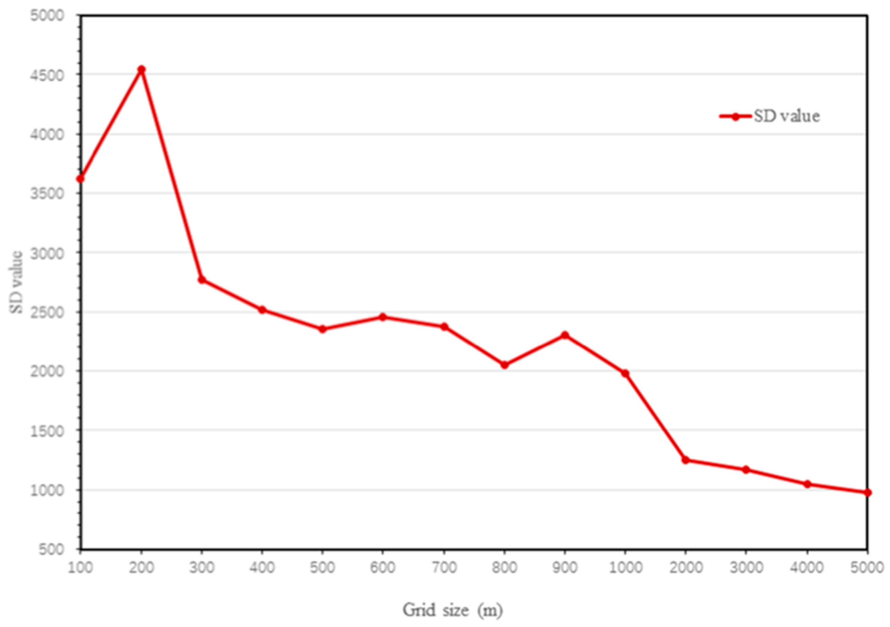
The SD values of 14 multiple-size gridded population distribution datasets were calculated in ArcGIS. We found that SD increased sharply from 100 m to 200 m, decreased quickly from 200 m to 300 m, fluctuated from 300 m to 800 m, slightly increased from 800 m to 900 m, decreased sharply from 900 m to 2000 m, and increased slowly before decreasing from 2000 m to 5000 m.
The 14 kinds of grid sizes, the SD value of the 200 m grid size was identified as the peak value. This further confirms that the 200 m grid size data effectively reveals the population distribution dispersion characteristics. Since SD value working on the whole image would eliminate some local discrepancy, the additional peak (corresponding grid size 900 m) obtained by both traditional and proposed ALV method was not obviously showed in Figure 10. However, we could also verify the validity of proposed method by SD value from the perspective of the whole image.
5. Conclusions
This paper proposed an improved ALV method for evaluating grid size suitability and tested it in a Chinese province by comparison with the traditional method. Grid size suitability evaluations must take into account the study area features and the research goal from the angle of usage requirements. Based on these considerations, the proposed method allows for the most suitable grid size to be chosen while the expected spatial characteristics are expressed effectively.
To establish the proposed method, we selected different window sizes and ensured they covered the same actual ground areas of different population distribution datasets. The ALV values calculated by the proposed method in this manner were more comparable and objective than those calculated by the traditional method. The results based on Anhui Province indicated that 200 m grid size most accurately expresses the study area’s population density discrepancies. In other words, the smallest grid size is not always most effective.
Errors in the actual ground areas could not be fully eliminated due to calculation restrictions but could be minimized by adjusting the moving window’s number of rows and columns. The errors affected the line graph features to some extent, but did not affect the main trends in ALV values. The line graph based on the proposed ALV method showed more regular and expected features with a clearer peak than the traditional method. It is worth noting that the improvements proposed here would be more effective in areas with heterogenous distribution features, as the new method works by distinguishing the differences between grid cells. Besides, the proposed method would not be able to choose the best grid size at one time while multiple locations of different spatial scales with different features of distribution were being studied.
In practice, the proposed method could be useful in enhancing the application level of grid size suitability research. Despite the limitation of study areas with heterogenous distribution features, we found the method to be effective and valuable both in theory and application. Unearthing the essential laws of the ALV method based on grid cell characteristics is an important research direction. Influence caused by terrain height and data should be taken into account in further research. The proposed method also merits further improvements in regards to its adaptability to multiple locations with different kinds of distribution characteristics.
Acknowledgments
This research was jointly supported by the Project of the National Natural Science Foundation of China (41771460, 41271173).
Author Contributions
Dong Huang analyzed the data and wrote the paper; Xiaohuan Yang, Nan Dong, and Hongyan Cai modified the paper.
Conflicts of Interest
The authors declare no conflict of interest.
References
- Du, G.; Zhang, S.; Zhang, Y. Analyzing spatial auto-correlation of population distribution: A case of Shenyang city. Geogr. Res. 2007, 26, 383–390. [Google Scholar]
- Bai, Z.; Wang, J.; Yang, F. Research progress in spatialization of population data. Prog. Geogr. 2013, 32, 1692–1702. [Google Scholar]
- Patel, N.N.; Stevens, F.R.; Huang, Z.; Gaughan, A.E.; Elyazar, I.; Tatem, A.J. Improving large area population mapping using geotweet densities. Trans. GIS 2017, 21, 317–331. [Google Scholar] [CrossRef] [PubMed]
- Li, Y.; Yang, X.; Wang, J. Grid size suitability of population spatial distribution in shandong province based on landscape ecology. Geogr. Geo-Inf. Sci. 2014, 30, 97–100. [Google Scholar]
- Mennis, J. Generating surface models of population using dasymetric mapping. Prof. Geogr. 2003, 55, 31–42. [Google Scholar]
- Du, G.; Zhang, S.; Zhang, Y. Analyzing scale effects of population density with shenyang city as a case. J. Grad. Sch. Chin. Acad. Sci. 2007, 24, 186–192. [Google Scholar]
- Ming, D.; Wang, Q.; Yang, J. Spatial scale of remote sensing image and selection of optimal spatial resolution. J. Remote Sens. 2008, 12, 529–537. [Google Scholar]
- Ye, J.; Yang, X.; Jiang, D. The grid scale effect analysis on town leveled population statistical data spatialization. J. Geo-Inf. Sci. 2010, 12, 40–47. [Google Scholar] [CrossRef]
- Wang, P.; Shi, P.; Wei, W.; Zhang, S. Grid scale effect and spatialization of population density based on the characteristic of spatial autocorrelation in Shiyang River Basin. Adv. Earth Sci. 2012, 27, 1363–1372. [Google Scholar]
- Woodcock, C.E.; Strahler, A.H. The factor of scale in remote sensing. Remote Sens. Environ. 1987, 21, 311–332. [Google Scholar] [CrossRef]
- Bocher, P.K.; McCloy, K.R. The fundamentals of average local variance—Part I: Detecting regular patterns. IEEE Trans. Image Process. 2006, 15, 300–310. [Google Scholar] [CrossRef] [PubMed]
- Ming, D.; Li, J.; Wang, J.; Zhang, M. Scale parameter selection by spatial statistics for geobia: Using mean-shift based multi-scale segmentation as an example. ISPRS J. Photogramm. Remote Sens. 2015, 106, 28–41. [Google Scholar] [CrossRef]
- Atkinson, P.M.; Curran, P.J. Choosing an appropriate spatial resolution for remote sensing investigations. Photogramm. Eng. Remote Sens. 1997, 63, 1345–1351. [Google Scholar]
- Curran, P.J. The semivariogram in remote sensing: An introduction. Remote Sens. Environ. 1988, 24, 493–507. [Google Scholar] [CrossRef]
- Woodcock, C.E.; Strahler, A.H.; Jupp, D.L.B. The use of variograms in remote sensing: I. Scene models and simulated images. Remote Sens. Environ. 1988, 25, 349–379. [Google Scholar] [CrossRef]
- Qin, C.; Hu, X. Review on scale-related researches in grid-based digital terrain analysis. Geogr. Res. 2014, 32, 270–283. [Google Scholar]
- Hu, X.; Qin, C. Effects of different topographic attributes on determining appropriate dem resolution. Prog. Geogr. 2014, 33, 50–56. [Google Scholar]
- Zheng, H. Study the Fundamentals of Detecting Spatial Pattern in Remote Sensing Images by Comparing Average Local Variance with Semi-Variograms. Ph.D. Thesis, Northeast Institute of Geography and Agroecology, University of Chinese Academy of Sciences, Jilin, China, 2014. [Google Scholar]
- Mccloy, K.R.; Bøcher, P.K. Optimizing image resolution to maximize the accuracy of hard classification. Photogramm. Eng. Remote Sens. 2007, 73, 893–903. [Google Scholar] [CrossRef]
- Wang, Y.Q.; Liu, W.; Wang, Y. Image quality acessment based on local variance and structure similarity. J. Optoelectron. Laser 2008, 19, 1546–1553. [Google Scholar]
- Bocher, P.K.; McCloy, K.R. The fundamentals of average local variance—Part II: Sampling simple regular patterns with optical imagery. IEEE Trans. Image Process. 2006, 15, 311–318. [Google Scholar] [CrossRef] [PubMed]
- Schmidt, J.; Andrew, R. Multi-scale landform characterization. Area 2005, 37, 341–350. [Google Scholar] [CrossRef]
- Yang, X.; Zhang, S.; Xia, Y. Coupling pattern evolution of “population-economy-space-environment” in the counties of anhui province. Geogr. Geo-Inf. Sci. 2017, 33, 81–126. [Google Scholar]
- Yang, X.; Huang, Y.; Dong, P.; Jiang, D.; Liu, H. An updating system for the gridded population database of china based on remote sensing, gis and spatial database technologies. Sensors (Basel) 2009, 9, 1128–1140. [Google Scholar] [CrossRef] [PubMed]
- Lloyd, C.D.; Atkinson, P.M. Scale and the spatial structure of landform: Optimising sampling strategies with geostatistics. In Proceedings of the 3rd International Conference on GeoComputation, Bristol, UK, 17–19 September 1998. [Google Scholar]
- Dong, N.; Yang, X.; Cai, H. Research progress and perspective on the spatialization of population data. J. Geo-Inf. Sci. 2016, 1295–1304. [Google Scholar] [CrossRef]
- Dong, N.; Yang, X.; Cai, H.; Xu, F. Research on grid size suitability of gridded population distribution in urban area: A case study in urban area of Xuanzhou district, China. PLoS ONE 2017, 12, e0170830. [Google Scholar] [CrossRef] [PubMed]
- Dragut, L.; Eisank, C. Object representations at multiple scales from digital elevation models. Geomorphology (Amst) 2011, 129, 183–189. [Google Scholar] [CrossRef] [PubMed]
Figure 1.
Grid population distribution of Anhui Province at 100 m, 500 m, 1000 m, and 5000 m grid, respectively.
Figure 1.
Grid population distribution of Anhui Province at 100 m, 500 m, 1000 m, and 5000 m grid, respectively.
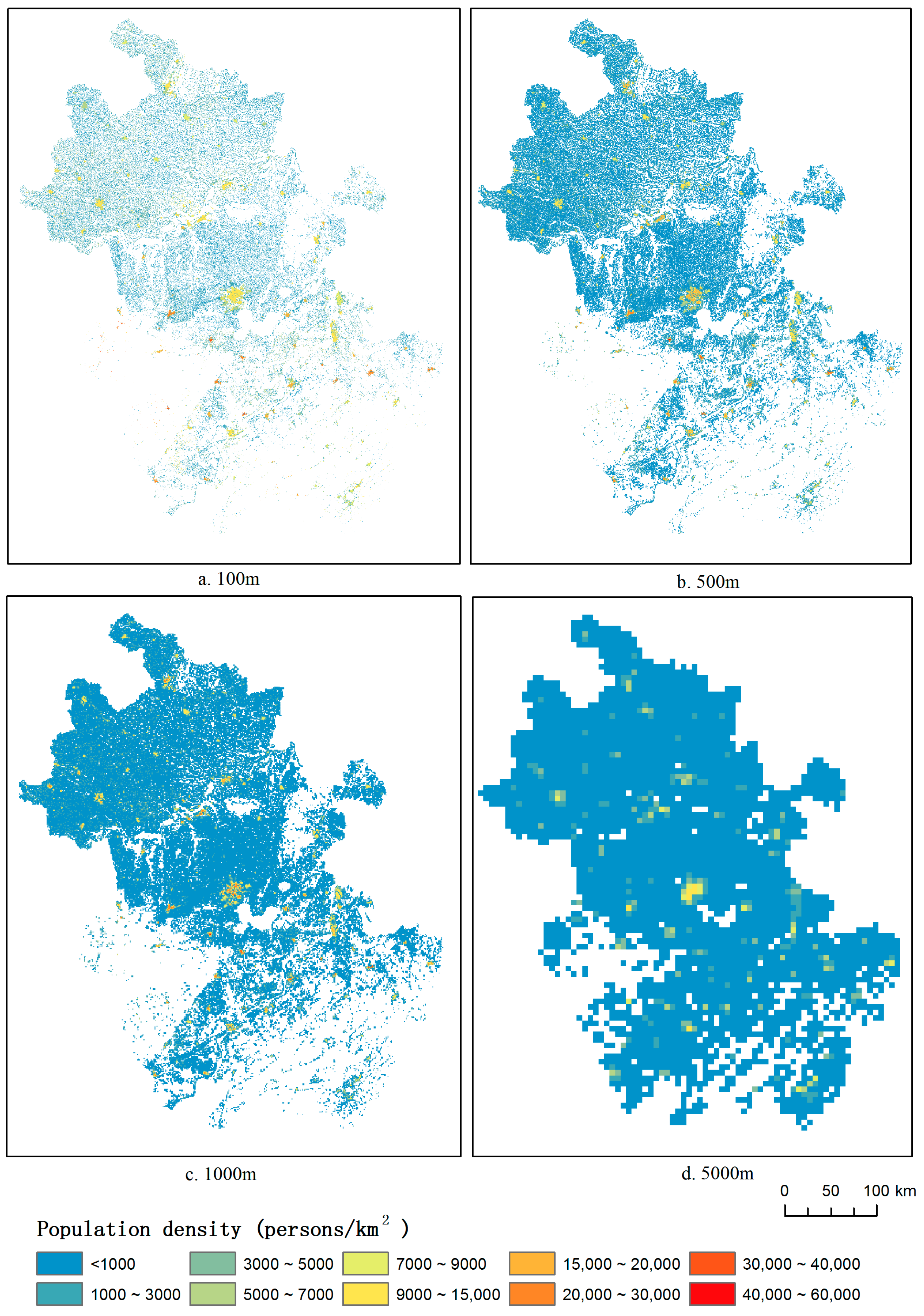
Figure 2.
Average local variance (ALV) method applied to grid size suitability evaluation.
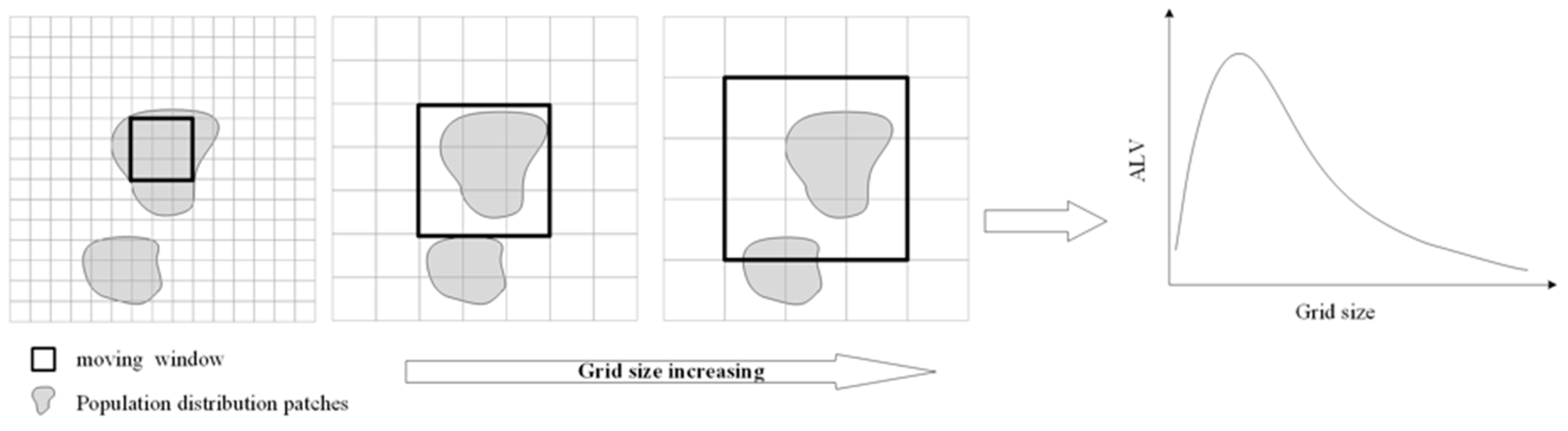
Figure 3.
Proposed ALV method applied to grid size suitability evaluation.

Figure 4.
Local variance data based on 3 × 3 moving windows of varying grid size.

Figure 5.
ALV value variations with grid size among different window sizes.
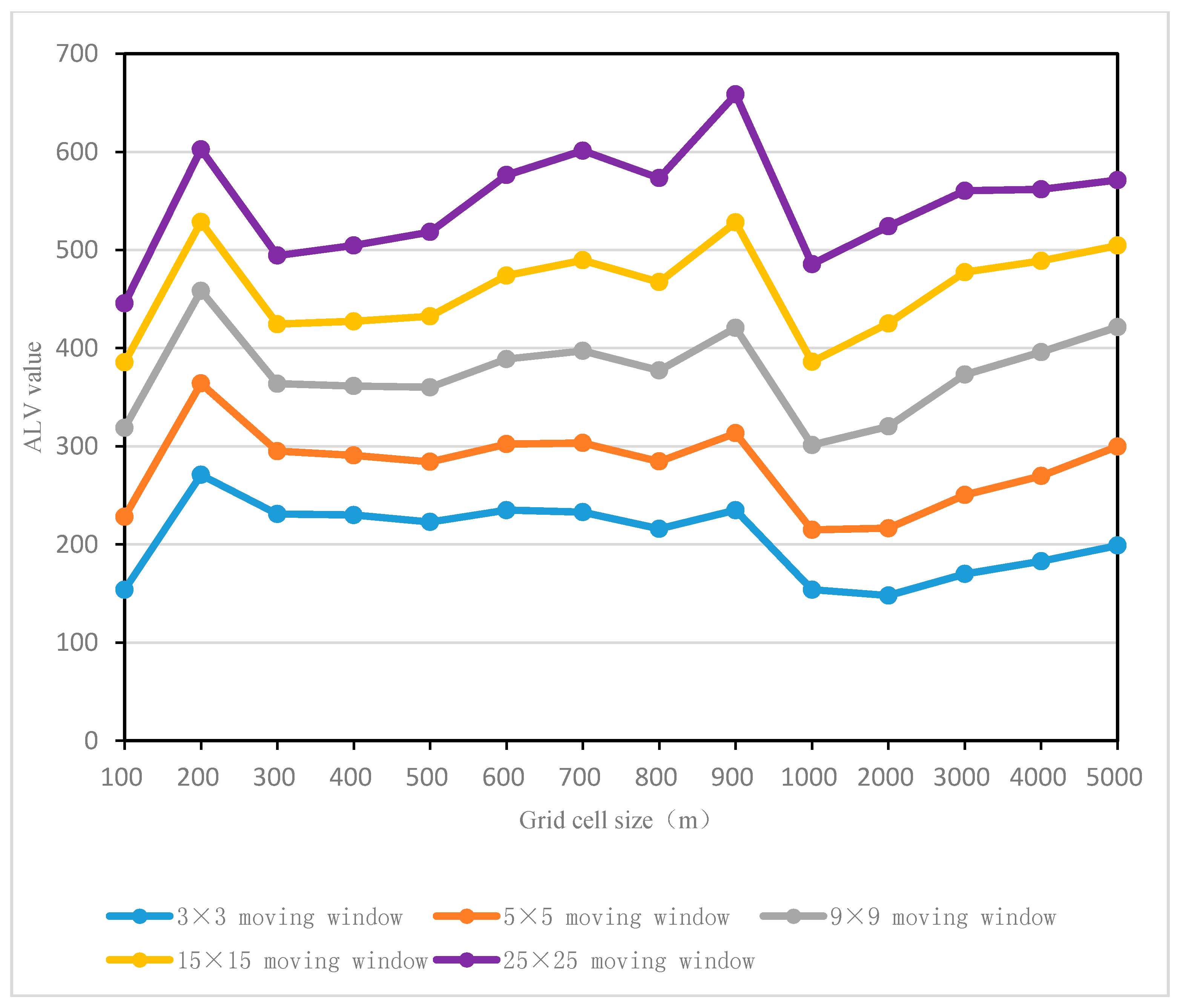
Figure 6.
Local variance data based on 225 km2 moving windows of varying grid size.

Figure 7.
Variations in ALV value with grid size based on different ground areas.
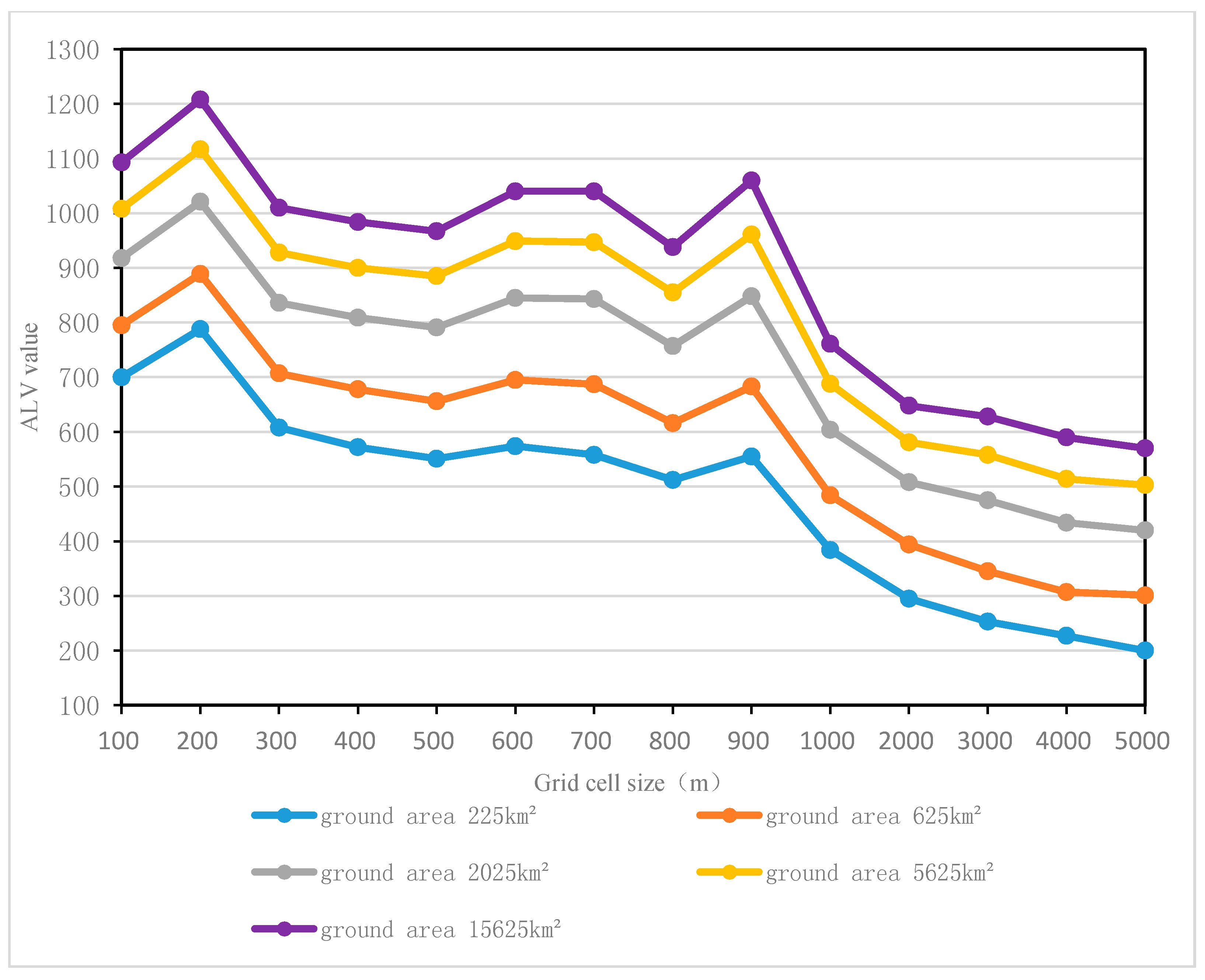
Figure 8.
ALV values with uniform grid size and increasing window size or ground area.

Figure 9.
Grid population distribution of local region at 100 m–900 m versus 1000 m–5000 m grid.

Figure 10.
SD values with varying grid size.

Table 1.
Data sources.
| Name | Time | Datatype | Scale/Resolution | Data Resources |
|---|---|---|---|---|
| Census data | 2010 | Excel | County level | State Bureau of Statistics of China |
| Boundary of counties | 2010 | vector | 1:1,000,000 | Resources and Environmental Scientific Data Center (RESDC), Chinese Academy of Sciences (CAS) |
| Boundary of townships | 2010 | vector | 1:1,000,000 | RESDC |
| Land use | 2010 | grid | 1 km × 1 km | RESDC |
Table 2.
Changes in actual ground area caused by different grid sizes.
| Grid Size (m) | Moving Window Size | Actual Ground Area (m2) |
|---|---|---|
| 100 | 3 × 3 | 90,000 |
| 200 | 3 × 3 | 360,000 |
| 300 | 3 × 3 | 810,000 |
Table 3.
Theoretical and actual window sizes corresponding to theoretical and actual ground areas; area errors of different grid sizes.
Table 3.
Theoretical and actual window sizes corresponding to theoretical and actual ground areas; area errors of different grid sizes.
| Theoretical Ground Area (km2) | Grid Size (m) | Theoretical Window Size | Actual Window Size | Actual Ground Area (km2) | Area Error (%) |
|---|---|---|---|---|---|
| 225 | 100 | 150 × 150 | 151 × 149 | 224.99 | 0.00 |
| 200 | 75 × 75 | 75 × 75 | 225 | 0.00 | |
| 300 | 50 × 50 | 51 × 49 | 224.91 | 0.04 | |
| 400 | 37.5 × 37.5 | 37 × 37 | 219.04 | 2.65 | |
| 500 | 30 × 30 | 31 × 29 | 224.75 | 0.11 | |
| 600 | 25 × 25 | 25 × 25 | 225 | 0.00 | |
| 700 | 21.43 × 21.43 | 21 × 21 | 216.09 | 3.96 | |
| 800 | 18.75 × 18.75 | 19 × 19 | 231.04 | 2.68 | |
| 900 | 16.66 × 16.66 | 17 × 17 | 234.09 | 4.04 | |
| 1000 | 15 × 15 | 15 × 15 | 225 | 0.00 | |
| 2000 | 7.5 × 7.5 | 9 × 7 | 252 | 12.00 | |
| 3000 | 5 × 5 | 5 × 5 | 225 | 0.00 | |
| 4000 | 3.75 × 3.75 | 5 × 3 | 240 | 6.67 | |
| 5000 | 3 × 3 | 3 × 3 | 225 | 0.00 | |
| 625 | 100 | 250 × 250 | 251 × 249 | 624.99 | 0.00 |
| 200 | 125 × 125 | 125 × 125 | 625 | 0.00 | |
| 300 | 83.33 × 83.33 | 83 × 83 | 620.01 | 0.80 | |
| 400 | 62.5 × 62.5 | 63 × 63 | 635.04 | 1.61 | |
| 500 | 50 × 50 | 51 × 49 | 624.75 | 0.04 | |
| 600 | 41.67 × 41.67 | 43 × 41 | 634.68 | 1.55 | |
| 700 | 35.71 × 35.71 | 37 × 35 | 634.55 | 1.53 | |
| 800 | 31.25 × 31.25 | 31 × 31 | 615.04 | 1.59 | |
| 900 | 27.78 × 27.78 | 29 × 27 | 634.23 | 1.48 | |
| 1000 | 25 × 25 | 25 × 25 | 625 | 0.00 | |
| 2000 | 12.5 × 12.5 | 13 × 13 | 676 | 8.16 | |
| 3000 | 8.33 × 8.33 | 9 × 7 | 567 | 9.28 | |
| 4000 | 6.25 × 6.25 | 7 × 5 | 560 | 10.40 | |
| 5000 | 5 × 5 | 5 × 5 | 625 | 0.00 | |
| 2025 | 100 | 450 × 450 | 451 × 449 | 2024.99 | 0.00 |
| 200 | 225 × 225 | 225 × 225 | 2025 | 0.00 | |
| 300 | 150 × 150 | 151 × 149 | 2014.91 | 0.50 | |
| 400 | 112.5 × 112.5 | 113 × 113 | 2043.04 | 0.89 | |
| 500 | 90 × 90 | 91 × 89 | 2024.75 | 0.01 | |
| 600 | 75 × 75 | 75 × 75 | 2025 | 0.00 | |
| 700 | 64.29 × 64.29 | 65 × 65 | 2070.25 | 2.23 | |
| 800 | 56.25 × 56.25 | 57 × 55 | 2006.4 | 0.92 | |
| 900 | 50 × 50 | 51 × 49 | 2024.19 | 0.04 | |
| 1000 | 45 × 45 | 45 × 45 | 2025 | 0.00 | |
| 2000 | 22.5 × 22.5 | 23 × 23 | 2116 | 4.49 | |
| 3000 | 15 × 15 | 15 × 15 | 2025 | 0.00 | |
| 4000 | 11.25 × 11.25 | 11 × 11 | 1936 | 4.40 | |
| 5000 | 9 × 9 | 9 × 9 | 2025 | 0.00 | |
| 5625 | 100 | 750 × 750 | 751 × 749 | 5624.99 | 0.00 |
| 200 | 375 × 375 | 375 × 375 | 5625 | 0.00 | |
| 300 | 250 × 250 | 251 × 249 | 5624.91 | 0.00 | |
| 400 | 187.5 × 187.5 | 187 × 187 | 5595.04 | 0.53 | |
| 500 | 150 × 150 | 151 × 149 | 5624.75 | 0.00 | |
| 600 | 125 × 125 | 125 × 125 | 5625 | 0.00 | |
| 700 | 107.14 × 107.14 | 107 × 107 | 5610.01 | 0.27 | |
| 800 | 93.75 × 93.75 | 95 × 93 | 5654.4 | 0.52 | |
| 900 | 83.33 × 83.33 | 83 × 83 | 5580.09 | 0.80 | |
| 1000 | 75 × 75 | 75 × 75 | 5625 | 0.00 | |
| 2000 | 37.5 × 37.5 | 37 × 37 | 5476 | 2.65 | |
| 3000 | 25 × 25 | 25 × 25 | 5625 | 0.00 | |
| 4000 | 18.75 × 18.75 | 19 × 17 | 5168 | 8.12 | |
| 5000 | 15 × 15 | 15 × 15 | 5625 | 0.00 | |
| 15,625 | 100 | 1250 × 1250 | 1251 × 1249 | 15,624.99 | 0.00 |
| 200 | 625 × 625 | 625 × 625 | 15,625 | 0.00 | |
| 300 | 416.66 × 416.66 | 417 × 417 | 15,650.01 | 0.16 | |
| 400 | 312.5 × 312.5 | 313 × 313 | 15,675.04 | 0.32 | |
| 500 | 250 × 250 | 251 × 249 | 15,624.75 | 0.00 | |
| 600 | 208.33 × 208.33 | 209 × 207 | 15,574.68 | 0.32 | |
| 700 | 178.57 × 178.57 | 179 × 177 | 15,524.67 | 0.64 | |
| 800 | 156.25 × 156.25 | 157 × 155 | 15,574.4 | 0.32 | |
| 900 | 138.89 × 138.89 | 139 × 139 | 15,650.01 | 0.16 | |
| 1000 | 125 × 125 | 125 × 125 | 15,625 | 0.00 | |
| 2000 | 62.5 × 62.5 | 63 × 61 | 15,372 | 1.62 | |
| 3000 | 41.67 × 41.67 | 43 × 41 | 15,867 | 1.55 | |
| 4000 | 31.25 × 31.25 | 33 × 31 | 16,368 | 4.76 | |
| 5000 | 25 × 25 | 25 × 25 | 15,625 | 0.00 |
© 2017 by the authors. Licensee MDPI, Basel, Switzerland. This article is an open access article distributed under the terms and conditions of the Creative Commons Attribution (CC BY) license (http://creativecommons.org/licenses/by/4.0/).
Share and Cite
MDPI and ACS Style
Huang, D.; Yang, X.; Dong, N.; Cai, H. Evaluating Grid Size Suitability of Population Distribution Data via Improved ALV Method: A Case Study in Anhui Province, China. Sustainability 2018, 10, 41. https://doi.org/10.3390/su10010041
AMA Style
Huang D, Yang X, Dong N, Cai H. Evaluating Grid Size Suitability of Population Distribution Data via Improved ALV Method: A Case Study in Anhui Province, China. Sustainability. 2018; 10(1):41. https://doi.org/10.3390/su10010041
Chicago/Turabian StyleHuang, Dong, Xiaohuan Yang, Nan Dong, and Hongyan Cai. 2018. "Evaluating Grid Size Suitability of Population Distribution Data via Improved ALV Method: A Case Study in Anhui Province, China" Sustainability 10, no. 1: 41. https://doi.org/10.3390/su10010041
Note that from the first issue of 2016, this journal uses article numbers instead of page numbers. See further details here.