Motives of Stock Option Incentive Design, Ownership, and Inefficient Investment

Abstract

This paper analyzes the effects of stock option incentives on inefficient investment. Specifically, based on the motive of design, we divide stock option incentives into incentive-driven and welfare-driven incentives. Our research is based on the panel data of 511 Chinese listed companies that declared stock option incentives from 2010 to 2014, including both incentive-driven and welfare-driven incentives. Our research shows that different types of stock option incentives have different effects on inefficient investment. Generally, incentive-driven stock option incentives reduce inefficient investment, whereas welfare-driven stock option incentives do not reduce inefficient investment, but increase it. However, there is a weakening effect in state-owned enterprises due to two opposite factors, numerous restrictions and more self-interested managers. Additionally, the paper provides implications that some stock options are manipulated by managers in the designing stage in order to pursue self-interests, and therefore monitoring abnormal share price movement and performance hurdles is important to safeguard the wealth of shareholders and promote effective motivation for managers.

1. Introduction

Agency problems are among the corporate governance problems many big companies face [1]. Agency problems between managers and shareholders can cause many problems, one of which is inefficient investment [2]. Managers may invest in projects for their own interests, not for shareholders’ interests [3]. Under a rational and perfect information market assumption, firms invest efficiently in projects with positive net present value (NPV) [4]. However, in practice, efficiency is different for each investment. Investments with low efficiency are called inefficient investments. Inefficient investments include overinvestment and underinvestment, both of which reflect suboptimal investment decisions.

Theoretically, stock option incentives are a way to reduce the agency problem and thereby reduce inefficient investment. Stock option incentives can align the interests between shareholders and managers, thereby reducing the agency problem [1,5,6,7]. Souder and Shaver (2010) and Agrawal and Mandelker (1987) proved that managers are likely to pursue long-term oriented efficient investments when receiving managerial stock options [5,8].

However, Jensen et al. (2004) argued that stock option incentives cannot provide an effective tool to motivate employees and instead becomes a tool manipulated by directors to earn benefit for themselves [9]. Veenman et al. (2011) argued that an asymmetric payoff structure of stock options may lead to managerial opportunistic behavior, which cannot improve investment efficiency [10]. In addition, a high level of share option holding will lead to managers’ myopia in investment. In order to prove their ability, managers tend to overinvest in the short term [11,12]. Based on 257 Chinese listed manufacturing companies, Wang et al. (2013) found that overinvestment is positively related with stock option incentives [13]. Stock option incentives cannot effectively reduce inefficient investment and cannot reduce the agency problem.

Therefore, there is no consistent conclusion about the relationship between stock option incentives and inefficient investment. One of the most important elements affects the effectiveness of stock option incentives, but little research has investigated the motives of stock option incentive design. In order to solve such a problem, this paper investigates the individual characteristics of stock option incentives. Some stock option incentives show features of shorter duration and lower vesting conditions, especially for companies with a powerful CEO who is skeptical [12,14]. Therefore, not all stock option incentives are designed to motivate employees and some of them are manipulated by CEOs to earn their own profits.

China has a large capital market and stock market to investigate. In addition, unlike other countries, it has its own economic structure. From the beginning of new China, a large number of state-owned enterprises have been set up, and they constitute a large proportion of total investment. It is reported that the portion of state-owned enterprise investment in total fixed investment was 41.1% in 2014. Because of abnormal ownership and government control, state-owned enterprises face problems of company-paid consumption, self-pay, self-welfare, etc. However, in responding to such problems, state-owned enterprises are also under restrictive regulations. Therefore, further investigation into the motives of stock option incentive design and the real effects of stock option incentives on inefficient investment of state-owned enterprises is necessary.

Stock option incentives have a history of nearly 30 years in the world, and many countries have executed different types of stock option incentives to resolve the agency problem. Stock option incentives originated in the USA and became a popular method of employee compensation. Among large USA listed companies, employee stock option incentives constitute more than 50% of total compensation. In India, it is reported that 43% of information technology (IT) companies have given stock options to more than 90% of the employees, and 17% of non-IT companies have done so. More than 75% of non-IT companies offer stock options to only senior and middle-management employees. However, stock option incentives also bring some problems, such as manipulation of the company’s performance and share price. For example, Michael Rand, the CFO of Beazer Homes, manipulated the profit of the company to earn himself USD 63 million, and Kenneth Lay, the CEO of Enron Corporation, published bogus news to manipulate share prices.

Stock option incentives have been popularized in China in the past 10 years. Since the beginning of the 1990s, stock option incentives were first used by Chinese listed companies to motivate managers. The enactment of “Administrative measures for stock option incentive of Chinese listed companies” increased the number of companies declaring stock option incentives in 2006. Nowadays, stock option incentives are mostly used by listed companies and new small and medium enterprises (SMEs).

This paper can be divided into six parts. First, the paper describes the background of this problem and gives a literature review of relevant research. Second, it analyzes the relevant theories about stock options and inefficient investment and presents a hypothesis based on theoretical analysis. Third, models to calculate inefficient investment and examine the relationship between stock option incentives and inefficient investment are set up. Fourth, it gives the empirical results of the model. Fifth, based on an alternative way of grouping stock option incentives, the paper conducts a robustness test of the results. Finally, it gives conclusions and a discussion.

To be specific, this paper is designed to collect data of 511 companies that declared stock option incentives in 2010–2014. After that, stock option incentives are divided based on cumulative abnormal return, into incentive-driven and welfare-driven groups. We also investigate the characteristics of individual stock option incentives, including vesting conditions and validity periods, to reclassify stock option incentives in a robustness check. Then, we examine the relationship between stock option incentives and inefficient investment regarding two types of stock option incentives. Further, as state-owned enterprises do not have owners, are controlled by government, and have political goals besides economic goals, we investigate and compare the relationship between stock option incentives and inefficient investment of state-owned companies versus private-owned companies. The conclusion is that the effects of different types of stock option incentives on inefficient investment are different. Incentive-driven stock option incentives can reduce inefficient investment, whereas welfare-driven stock option incentives cannot reduce, and may even increase, inefficient investment. This phenomenon is weak in state-owned companies due to two opposite factors: numerous restrictions and more self-interested managers.

The contributions of the paper can be concluded in two points. First, the paper divides stock option incentives based on design motive into incentive-driven and welfare-driven incentives and then investigates their relationships with inefficient investment. The paper analyzes the characteristics of every stock option incentive and gives a more rational conclusion instead of mixing all types of stock option incentives together, which cannot differentiate the effects of the different types on inefficient investment. Second, the paper also investigates different types of stock option incentives in state-owned enterprises to see whether the effects are the same with different types of company ownership. The paper’s main innovation is that it tries to describe the relationship between stock option incentives and inefficient investment from a new aspect, which is the motive of stock option incentive design. It examines the effects of different types of stock option incentives on inefficient investment and identifies the self-interest behavior of managers in designing stock option incentives.

2. Theoretical Analysis and Hypothesis

In the past 20 years, with the scandals of Enron and WorldCom, the effects and intentions of stock option incentives are in doubt. Researchers hold different opinions on stock option incentives. Most researchers stand up for the effectiveness of stock option incentives [15,16,17]. Mainly, there are two advantages of stock option incentives. First, they can solve information asymmetry. The result of information asymmetry is that shareholders cannot easily evaluate investment decisions made by managers. Therefore, shareholders apply stock option incentives, which lets the market evaluate investment decisions [18]. Second, stock option incentives can motivate managers to become long-term oriented and avoid the myopia problem [16]. Stock option incentives can solve the agency problem by motivating managers to choose investment projects that provide extra profits from long-term share price increases and making the sunken investment costs relevant from the manager’s perspective [15,19].

However, in contrast to the above opinions, some researchers doubt the effectiveness of stock option incentives. Canil and Karpavičius held that employee stock options are granted for other purposes and proceeds they bring may be sources for company financing [20]. Tzioumis denied the stock option incentive by finding that the older the managers are, the lower the shares they will receive, which cannot solve the myopia problem [21]. Chaigneau stated that stock option incentives have a convex effect in performance, which means there is a suboptimal effect when the agent has mean-variance preferences [22]. Vintilă and Gherghina concluded that there was a negative influence of employee organization ownership on firm value [23]. Other researchers stated that the design of stock option incentives should include some non-incentive considerations. There are mainly four non-incentive considerations. From the perspective of the company, first, in order to save money, companies use stock option incentives to motivate managers rather than salary incentives. Second, stock option incentives bring tax advantages [24]. From the perspective of managers, third, stock option incentives may be manipulated by managers by setting shorter durations and lower performance hurdles [25]. Finally, managers may misreport earnings to gain private benefit by disclosing bad news before declaring stock option incentives to get a lower exercise price [26,27].

Considering the above non-incentive considerations, the paper divides stock option incentives into incentive-driven and welfare-driven stock options. Incentive-driven stock option incentives should be designed with long validity periods and high-performance hurdles and without abnormal share price movements to cultivate a long-term horizon for managers when considering the company’s value. Under such circumstances, it is difficult for managers to invest inefficiently.

However, mangers with overcontrolled power will tend to design stock option incentives with shorter validity periods and lower performance hurdles to earn private benefits. Besides this method, more managers also manipulate share prices to earn private benefits. Usually, the granting of stock options should be a formal and time-sensitive process, and therefore the option exercise price should be equal to the market price at the time of the grant [28]. Since managers know the declaration date in advance, some opportunistic managers will manipulate share prices before the declaration date of the stock option incentive and release some bad news to get a lower exercise price, and release good news after the declaration date, thereby maximizing the value of options [29,30]. These are called welfare-driven stock option incentives. In order to examine the influence of the two types of stock option incentives on inefficient investment, we put forward assumptions H₁ and H₂.

H₁: Incentive-driven stock option incentives will reduce inefficient investment.

H₂: Welfare-driven stock option incentives will increase inefficient investment.

In China, state-owned enterprises account for not only a large proportion of investment, but also a fast growth rate in investment. It is reported that the portion of state-owned enterprises in total fixed investment from 2009 to 2014 was 50.1%, 47.3%, 43.4%, 39%, 45.1%, and 41.1%, respectively, each year. However, because of abnormal ownership and government control, state-owned enterprises face problems of company-paid consumption, self-pay, self-welfare, etc. Managers of state-owned enterprises are likely to use nonmonetary ways to earn profit. Although managers of state-owned enterprises have more self-welfare possibilities, they are also subject to numerous regulations. Declarations of stock option incentives of state-owned enterprises should get permission from the State-owned Assets Supervision and Administration Commission, the China Securities Regulatory Commission, etc. In addition, according to methods of implementing stock option incentives in state-owned enterprises, they cannot exceed 30% of total remuneration; performance hurdles should include at least one indicator, including return for shareholders, capability of profit growth, or company earnings, and should not be lower than the average performance of the industry.

Most research has focused on whole samples, and less research has investigated state-owned enterprises specifically. It can be seen that the condition of state-owned enterprises is complex and there are two opposite factors affecting the motives of stock option incentive design. On the one hand, as the ultimate controller of state-owned enterprises is the country and shareholders do not supervise managers, state-owned enterprises are likely overcontrolled by managers to earn their own profit. On the other hand, state-owned enterprises face more regulations regarding stock option incentives to prevent self-welfare of managers. Therefore, it is necessary to investigate the effects of the two kinds of stock option incentives on inefficient investment in state-owned enterprises. We put forward assumptions H₃ and H₄.

H₃: In state-owned enterprises, incentive-driven stock option incentive plans will reduce inefficient investment.

H₄: In state-owned enterprises, welfare-driven stock option incentive plans will increase inefficient investment.

3. Research Design

3.1. Measurement of Variables

All the data comes from Wind database. We chose companies, except financial enterprises, that declared stock option incentives from the Shanghai and Shenzhen stock exchanges during 2010–2014. In order to measure the effect of stock option incentives on inefficient investment, inefficient investment is measured from 2011 to 2015.

3.1.1. Classification of Stock Option Incentives

After eliminating abnormal and terminated stock option incentives, 511 companies declared stock option incentives during 2010–2014.

There are two main methods to classify stock option incentives. First, we can classify them by their characteristics. Validity periods and performance hurdles are used to classify stock option incentives, and Qu Xin has applied this method to Australia listed companies [31]. However, in China, characteristics of stock option incentives show herd effects and just maintain the lowest requests from regulators. Most stock option incentives have similar validity periods and performance hurdles. Therefore, it is hard to classify them by validity period.

Second, cumulative abnormal return (CAR) is another way to classify stock option incentives. As specified by the China Securities Regulatory Commission, the exercise price of stock option incentives cannot be below the higher closing price of one day before the stock option incentive has been declared and average closing price of the previous 30 days before the stock option incentive has been declared. Therefore, closing price plays an important role in deciding exercise price. Denis et al. (2006) and Liu et al. (2014) found that irregular stock option incentives are related to abnormal share price movements [30,32]. Stock-based compensation is more sensitive to a company’s share prices, and therefore the managers with welfare-driven stock option incentives are likely to manipulate share prices [33]. Welfare-driven companies are likely to disclose bad news before the declaration date in order to get lower exercise prices, which, in turn, will lead to a negative CAR. Under such circumstances, there is downward earnings management before the declaration date to maximize the value of option grants [34].

In this paper, the second method is chosen to classify stock option incentives, and we also use the first method to reclassify stock option incentives in a robustness test. In order to focus on the movement of share prices related to the declaration of stock option incentives, we use the event study method to calculate CAR in the event window period (from 10 days before the declaration of stock option incentives to one day after the declaration).

Stock option incentives declared by companies are identified and declaration dates are recorded. Then, CAR is calculated for every company by using event study. We use the Capital Asset Pricing Model (CAPM) to estimate the cumulative abnormal return within an event window. The formulas are as follows:

$$E\left(R_{i,t}\right)={\alpha }_i+{\beta }_i\ast R_{m,t}+{\epsilon }_{i,t}$$

(1)

$$A{R}_{i,t}=R_{i,t}-E\left(R_{i,t}\right)$$

(2)

$$CA{R}_{\left(-10,0\right),i}={\displaystyle \sum }_{t=10}^{0}A{R}_{i,t}$$

(3)

3.1.2. Inefficient Investment

Inefficient investment includes overinvestment and underinvestment. Overinvestment means that enterprises invest in projects with negative NPV, whereas underinvestment means that enterprises do not invest in projects with positive NPV [35].

In terms of measuring inefficient investment, one popular model is the Richardson model, which has been applied by many scholars [36,37]. The Richardson model (see model (4)) is used to calculate the expected new investment of each company. Investment is divided into two parts, maintenance investment and new investment. Based on model (4), an investment expectation model is used to generate expected new investment, and the residual value between expected new investment and real new investment is inefficient investment. Overinvestment is defined as residual value higher than 0, whereas underinvestment is defined as residual value lower than 0 [38].

$$\begin{array}{ll}In{v}_{i,t}={\alpha }_0+{\alpha }_1& \ast Q_{i,t-1}+{\alpha }_2\ast Le{v}_{i,t-1}+{\alpha }_3\ast Cas{h}_{i,t-1}+{\alpha }_4\ast Stock{R}_{i,t-1}+{\alpha }_5\\ & \ast Ag{e}_{i,t-1}+{\alpha }_6\ast Siz{e}_{i,t-1}+{\alpha }_7\ast Ln{v}_{i,t-1}+{\displaystyle \sum }Year\\ & +{\displaystyle \sum }Industry+{\epsilon }_{i,t}\end{array}$$

(4)

3.1.3. Other Variables

Because our sample of companies comes from 16 industries, we have adjusted Tobin Q according to each industry membership when calculating Tobin Q for each company following the method described by Eisenberg et al. [39].

Table 1. Industry membership of selected sample.

Industry	2010	2011	2012	2013	2014
Manufacturing	42	57	61	105	91
Construction	4	2	1	4	2
Real estate	7	4	3	2	1
Mining	0	1	0	0	1
Electricity, heat production and supply	0	0	1	0	1
Information transmission, software and information technology services	11	14	11	14	17
Water resources, environment, and public facilities management	2	0	0	2	1
Health and social work	1	0	0	2	0
Wholesale and retail businesses	2	2	2	4	4
Hotels and catering services	0	1	0	0	0
Scientific research and technical services	0	1	1	2	3
Culture, sports, and entertainment	0	1	1	1	1
Leasing and business services	1	0	0	1	4
Agriculture, forestry, animal husbandry, and fishery	0	2	2	1	3
Transportation, storage, and postal services	0	0	1	2	0
Others	1	0	1	0	1
Total	71	85	85	140	130

shows industry membership of the selected sample.

The method to calculate adjusted Tobin Q is described as follows. The difference between firm Q ratio and the industry’s median Q ratio is ∆Q, while the industry-adjusted measure of Q (QAdj) is defined as follows:

QAdj = sign(∆Q) × sqrt(∆Q)

(5)

where sign(∆Q) is the sign of the difference between firm Q and the industry’s median Q, while sqrt(∆Q) is the square root of ∆Q. We decided to use median instead of mean because our data did not follow a normal distribution.

Table 2. Other variables.

QAdj	Industry-adjusted Tobin Q: Tobin Q = (share price × tradable shares + net asset value per share × nontradable shares)/total assets
Lev	Leverage: total liabilities/total assets
Cash	Cash: cash and cash equivalents/total assets
StockR	Stock return
Age	Number of years company is listed
Size	Size: ln(total assets)
Lnv	Inew = Itotal − Imaintenance = cash outflow of constructing fixed assets, intangible assets, and other long-term assets − cash inflow of disposing fixed assets, intangible assets, and other long-term assets + cash outflow of acquiring subsidiary and other operating units − cash inflow of acquiring subsidiary and other operating units − (depreciation of assets + amortization of intangible assets + amortization of long-term prepaid expenses)
Year	Dummy variable: from 2010–2014
Industry	Dummy variable: industries specified by stock exchange
Option	1 represents stock option incentive declared; 0 represents no stock option incentive
ROA	Return on assets: net profit/average assets
Gshare	Number of shares held by managers
OW	Ownership: 1 represents state-owned enterprises; 0 represents private-owned enterprises
OW× Option	Interaction terms of OW and Option and is defined as OW times Option.
Shrhfd5	Top five shareholders’ shareholding amount

shows the definitions of other variables.

3.2. Models

Model (6) and (7) are shown as follows. Model (6) is used to examine the relationship between stock option incentive and inefficient investment. Model (7) introduces two new variables: OW and OW × Option to investigate the relationship between stock option incentive and inefficient investment in state-owned enterprises.

$$\begin{array}{l}Overinvestment{\left(Underinvestment\right)}_{i,t}\\ ={\alpha }_0+{\alpha }_1\ast Optio{n}_{i,t-1}+{\alpha }_2\ast Q_{i,t-1}+{\alpha }_3\ast Le{v}_{i,t-1}+{\alpha }_4\ast Cas{h}_{i,t-1}\\ +{\alpha }_5\ast Stock{R}_{i,t-1}+{\alpha }_6\ast Ag{e}_{i,t-1}+{\alpha }_7\ast Siz{e}_{i,t-1}+{\alpha }_8\ast RO{A}_{i,t-1}\\ + {\alpha }_9\ast Gshar{e}_{i,t-1}+{\alpha }_{10}\ast Shrhfd{5}_{i,t-1}+{\displaystyle \sum }Year\\ +{\displaystyle \sum }Industry+{\epsilon }_{i,t}\end{array}$$

(6)

$$\begin{array}{l}Overinvestment{\left(Underinvestment\right)}_{i,t}\\ ={\alpha }_0+{\alpha }_1\ast Optio{n}_{i,t-1}+{\alpha }_2\\ \ast O{W}_{i,t-1}+{\alpha }_3\ast Optio{n}_{i,t-1}\ast O{W}_{i,t-1}+{\alpha }_4{Q}_{i,t-1}+{\alpha }_5\ast Le{v}_{i,t-1}+{\alpha }_6\\ \ast Cas{h}_{i,t-1}+{\alpha }_7\ast Stock{R}_{i,t-1}+{\alpha }_8\ast Ag{e}_{i,t-1}+{\alpha }_9\ast Siz{e}_{i,t-1}+{\alpha }_{10}\\ \ast RO{A}_{i,t-1}+{\alpha }_{11}\ast Gshar{e}_{i,t-1}+{\alpha }_{12}\ast Shrhfd{5}_{i,t-1}+{\displaystyle \sum }Year\\ +{\displaystyle \sum }Industry+{\epsilon }_{i,t}\end{array}$$

(7)

4. Empirical Results and Discussion

4.1. Descriptive Statistics

4.1.1. Classification of Stock Option Incentives

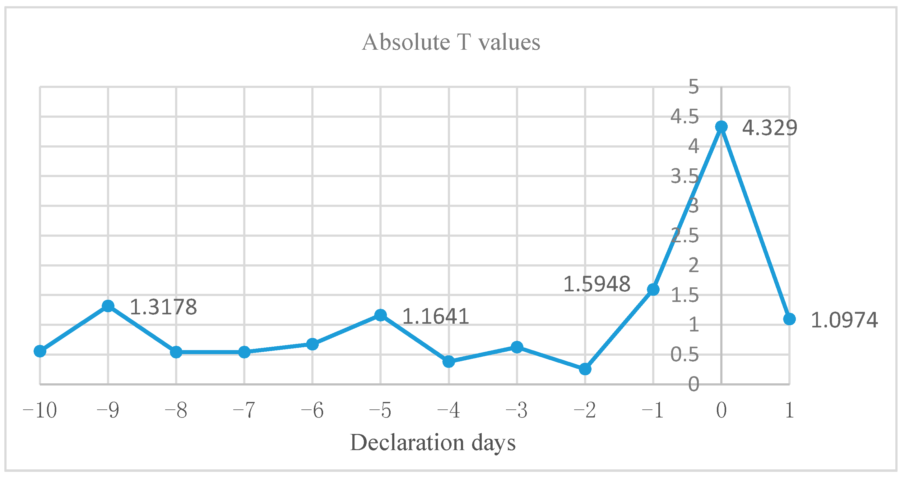
T test is applied to CAR calculated to verify the accuracy of the event window. From

Table 3. Market reaction to declaration (event window (−10, 1), estimation window (−110, −11)).

Declaration Day	Average AR (T Value)	Declaration Day	Average AR (T Value)
−10	−0.0015 (−0.5587)	−4	−0.0008 (−0.3822)
−9	−0.0031 (−1.3178) *	−3	−0.0014 (−0.6245)
−8	−0.0012 (−0.5428)	−2	−0.0005 (−0.2560)
−7	−0.003 (−0.1246)	−1	0.0037 (1.5948) **
−6	−0.0015 (−0.6754)	0	0.0121 (4.3290) ***
−5	−0.0029 (−1.1641) *	1	0.0030 (1.0974) *

Note: *, **, *** represent significance at levels of 10%, 5%, and 1%.

and Figure 1, it can be seen that closing price is statistically significant at day 1, 0, −1, −5, and −9. During these days, the difference between real closing price and expected closing price is significant, especially for the days close to the declaration date. Therefore, closing price fluctuates at day 1, 0, −1, −5, and −9 and event window is appropriate for event study.

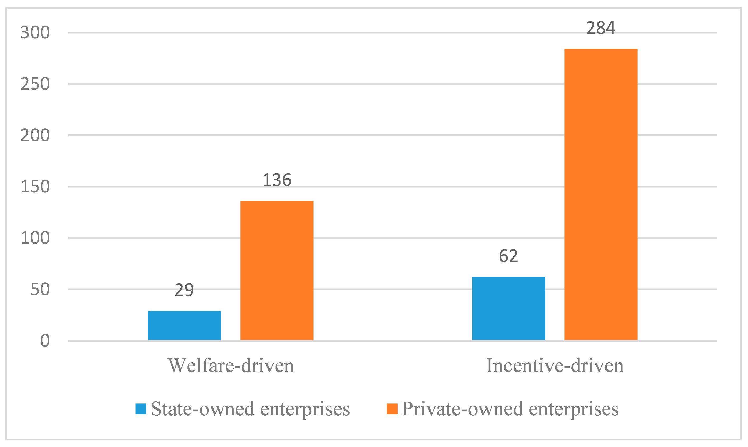
After classification, the companies are divided into incentive-driven and welfare-driven. As shown in

Table 4. Numbers of welfare-driven and incentive-driven companies.

	Welfare-Driven		Incentive-Driven		Total
	Number	Average CAR	Number	Average CAR
State-owned enterprises	29	−0.0898	62	0.0660	91
Private-owned enterprises	136	−0.1587	284	0.0804	420
Total	165		346		511

and Figure 2, 165 out of 511 companies are welfare-driven, whereas 346 companies are incentive-driven. Most stock option incentives are incentive-driven, but some are welfare-driven. Therefore, this conclusion proves that managers of some companies manipulate stock option incentives to earn their own profit. State-owned companies only occupy a small proportion of total companies that declared stock option incentives. This may be because declarations of stock option incentives in state-owned enterprises are concerned with the security of state assets and a lot of regulations need to be satisfied. Therefore, state-owned enterprises are reluctant to exercise stock option incentives. The proportion of incentive-driven and welfare-driven incentives is nearly the same for state-owned and private-owned enterprises. In terms of average CAR, it can be seen that the closing prices of private-owned enterprises fluctuate more wildly than those of state-owned enterprises. This may be because state-owned enterprises are regulated by numerous regulations and therefore there is less possibility to manipulate stock prices.

4.1.2. Inefficient Investment

Table 5. Descriptive statistics of inefficient investment.

		Overinvestment					Underinvestment
		N	Mean	Median	Max	Min	N	Mean	Median	Max	Min	Total
State-owned enterprises	Welfare-driven	18	0.0293	0.0226	0.0971	0.0018	11	−0.0345	−0.0241	−0.0085	−0.1405	29
	Incentive-driven	22	0.0719	0.0247	0.4291	0.0080	40	−0.0384	−0.0262	−0.0005	−0.1737	62
Private-owned enterprises	Welfare-driven	73	0.0545	0.0346	0.2438	0.0004	63	−0.0400	−0.0282	−0.0005	−0.1573	136
	Incentive-driven	137	0.0598	0.0353	0.4408	0.0004	147	−0.0471	−0.0359	−0.0014	−0.2243	284
Total		250					261					511

shows the descriptive statistics of inefficient investment. The numbers of overinvesting and underinvesting companies are nearly the same. Based on the mean and median of inefficient investment, the level in private-owned enterprises is higher than that in state-owned enterprises. Therefore, the problem of inefficient investment in private companies is more serious than in state-owned enterprises. In terms of overinvestment, the number of welfare-driven companies outweighs the incentive-driven ones, whereas, in terms of underinvestment, the number of incentive-driven companies outweighs welfare-driven ones. It can be concluded that the agency problem in overinvesting companies is more serious than in underinvesting companies.

In order to compare the differences in inefficient investment between companies with incentive-driven and welfare-driven stock option incentives, we apply the T test to overinvestment and underinvestment. From

Table 6. T test of inefficient investment between incentive-driven and welfare driven companies.

	Overinvestment		Underinvestment
	Incentive-Driven	Welfare-Driven	Incentive-Driven	Welfare-Driven
Mean	0.0615	0.049	−0.0453	−0.0392
Standard deviation	0.0056	0.0027	0.0017	0.0014
Sample	159	91	187	74
df	238		167
P	0.0701 *		0.1000 *
T	1.4796		1.6553

Note: * represent significance at levels of 10%.

, it can be concluded that inefficient investments of companies with incentive-driven and welfare-driven stock option incentives are significantly different at the 1% level. Therefore, different types of stock option incentives have different effects on inefficient investment and our research holds water.

4.1.3. Correlation Analysis

A correlation analysis was conducted on four groups: incentive-driven overinvestment, incentive-driven underinvestment, welfare-driven overinvestment, and welfare-driven underinvestment.

Table 7. Coefficient analysis of incentive-driven overinvestment group.

	Residual	Option	OW	OW × Option	QAdj	Leverage	Cash	StockR	Age	Size	ROA	Gshare	Shrhfd5
Residual	1
Option	−0.229 ***	1
OW	−0.125 ***	0.031	1
OW ×Option	0.139 ***	0.348 ***	0.594 ***	1
QAdj	0.145 ***	0.215 ***	0.005	0.032	1
Leverage	−0.016	0.011	0.234 ***	0.140 ***	−0.108 ***	1
Cash	−0.049	−0.122 ***	−0.114 ***	−0.110 ***	−0.031	−0.559 ***	1
StockR	0.053	0.072 **	0.015	0.071 **	0.302 ***	0.071 **	−0.081 **	1
Age	−0.036	0.135 ***	0.348 ***	0.242 ***	0.199 ***	0.441 ***	−0.4 ***	0.136 ***	1
Size	0.178 ***	0.185 ***	0.315 ***	0.239 ***	−0.012	0.54 ***	−0.349 ***	0.018	0.518 ***	1
ROA	0.015	−0.132 ***	−0.063 *	−0.032	0.064 *	−0.239 ***	0.226 ***	0.037	−0.251 ***	−0.232 ***	1
Gshare	0.015	0.016	−0.317 ***	−0.187 ***	−0.02	−0.349 ***	0.29 ***	0.003	−0.52 ***	−0.376 ***	0.202 ***	1
Shrhfd5	−0.047	−0.023	−0.019	−0.012	−0.044	−0.007	0.024	−0.11 ***	−0.093 ***	0.167 ***	−0.032	0.002	1

Note: *, **, *** represent significance at levels of 10%, 5%, and 1%.

shows results of the incentive-driven overinvestment group. From the table, it can be seen that stock option is negatively correlated with overinvestment (residual value), and this relationship also exists in state-owned enterprises. Overinvestment is severe in private-owned enterprises. Industry-adjusted Tobin Q is positively correlated with overinvestment. Company size is positively correlated with overinvestment.

Table 8. Coefficient analysis of incentive-driven under-investment group.

	Residual	Option	OW	OW×Option	QAdj	Leverage	Cash	StockR	Age	Size	ROA	Gshare	Shrhfd5
Residual	1
Option	0.163 ***	1
OW	0.153 ***	0.036	1
OW ×Option	0.165 ***	0.275 ***	0.692 ***	1
QAdj	−0.126 ***	0.176 ***	0.024	−0.016	1
Leverage	−0.031	0.039	0.26 ***	0.184 ***	−0.078 **	1
Cash	0.055 *	−0.197 ***	−0.117 ***	−0.097 ***	−0.058 *	−0.554 ***	1
StockR	−0.044	0.065 **	0.058 *	0.05	0.258 ***	0.113 ***	−0.109 ***	1
Age	−0.005	0.147 ***	0.309 ***	0.246 ***	0.287 ***	0.421 ***	−0.381 ***	0.156 ***	1
Size	0.19 ***	0.278 ***	0.319 ***	0.236 ***	−0.009	0.465 ***	−0.314 ***	0.005	0.443	1
ROA	0.045	−0.258 ***	−0.1 ***	−0.115 ***	−0.135 ***	−0.269 ***	0.38 ***	−0.004	−0.323 ***	−0.33 ***	1
Gshare	0.026	−0.044	−0.302 ***	−0.22 ***	−0.082 **	−0.348 ***	0.279 ***	−0.098 ***	−0.499 ***	−0.366 ***	0.219 ***	1
Shrhfd5	0.092 ***	0.062 *	0.063 *	0.038	0.05	−0.016	0.033	−0.058*	0.102 ***	0.23 ***	−0.095 ***	−0.026	1

Note: *, **, *** represent significance at levels of 10%, 5%, and 1%.

shows results of the incentive-driven underinvestment group. It can be seen that stock option is positively correlated with underinvestment (residual value), and the relationship also exists in state-owned enterprises. Underinvestment is more severe in private-owned enterprises. Industry-adjusted Tobin Q is negatively correlated with overinvestment. Cash is positively correlated with underinvestment. Company size is positively correlated with underinvestment. The amount of the top five shareholders’ shareholding is positively correlated with underinvestment.

Table 9. Coefficient analysis of welfare-driven overinvestment group.

	Residual	Option	OW	OW×Option	QAdj	Leverage	Cash	StockR	Age	Size	ROA	Gshare	Shrhfd5
Residual	1
Option	−0.034	1
OW	−0.12 **	−0.006	1
OW ×Option	−0.086 *	0.376 ***	0.624 ***	1
QAdj	0.115 **	0.219 ***	−0.071	−0.048	1
Leverage	0.094 *	0.082	0.173 ***	0.166 ***	−0.249 ***	1
Cash	−0.042	−0.23 ***	−0.023	−0.096 *	−0.03	−0.56 ***	1
StockR	0.066	0.217 ***	−0.061	0.065	0.251 ***	0.156 ***	−0.099 *	1
Age	0.051	0.269 ***	0.192 ***	0.215 ***	0.198 ***	0.451 ***	−0.347 ***	0.087 *	1
Size	−0.072	0.283 ***	0.293 ***	0.341 ***	−0.0008	0.534 ***	−0.336 ***	0.076	0.66 ***	1
ROA	−0.011	−0.221 ***	−0.176 ***	−0.199 ***	0.039	−0.233 ***	0.229 ***	0.009	−0.181 ***	−0.329 ***	1
Gshare	−0.04	−0.029	−0.269 ***	−0.169 ***	−0.053	−0.4 ***	0.286 ***	−0.01	−0.46 ***	−0.415 ***	0.125 **	1
Shrhfd5	−0.043	0.116 **	0.048	0.118 **	0.023	0.125 **	−0.051	0.01	0.067	0.292 ***	−0.225 ***	−0.224 ***	1

Note: *, **, *** represent significance at levels of 10%, 5%, and 1%.

shows results of the welfare-driven overinvestment group. It can be seen that stock option is positively correlated with underinvestment (residual value), and the relationship also exists in state-owned enterprises. Underinvestment is more severe in private-owned enterprises. Industry-adjusted Tobin Q is negatively correlated with overinvestment. Cash is positively correlated with underinvestment. Company size is positively correlated with underinvestment. The amount of the top five shareholders’ shareholding is positively correlated with underinvestment.

Table 10. Coefficient analysis of welfare-driven overinvestment group.

	Residual	Option	OW	OW×Option	QAdj	Leverage	Cash	StockR	Age	Size	ROA	Gshare	Shrhfd5
Residual	1
Option	0.014	1
OW	−0.043	0.083 *	1
OW ×Option	0.05	0.235 ***	0.75 ***	1
QAdj	−0.009	0.115 **	0.052	0.06	1
Leverage	−0.174 ***	0.192 ***	0.103 **	0.127 ***	−0.173 ***	1
Cash	0.099 **	−0.334 ***	−0.087 *	−0.166 ***	−0.101 **	−0.567 ***	1
StockR	−0.099 **	0.199 ***	−0.011	0.042	0.295 ***	0.095**	−0.161 ***	1
Age	0.136 ***	0.292 ***	0.13 ***	0.157 ***	0.268 ***	0.41 ***	−0.405 ***	0.145 ***	1
Size	−0.076	0.35 ***	0.102 **	0.135 ***	0.022	0.526 ***	−0.342 ***	0.028	0.568 ***	1
ROA	0.15 ***	−0.308 ***	−0.13 ***	−0.131 ***	−0.021	−0.381 ***	0.344	0.038	−0.202 ***	−0.281 ***	1
Gshare	−0.122 **	−0.11 **	−0.151 ***	−0.136 ***	−0.195 ***	−0.326 ***	0.259 ***	−0.138 ***	−0.506 ***	−0.39 ***	0.093 *	1
Shrhfd5	−0.045	0.018	0.031	−0.009	−0.009	0.066	0.059	−0.045	−0.053	0.236 ***	−0.186 ***	−0.124 **	1

Note: *, **, *** represent significance at levels of 10%, 5%, and 1%.

shows results of the welfare-driven underinvestment group. It can be seen that stock option is positively correlated with underinvestment (residual value), and the relationship also exists in state-owned enterprises. Underinvestment is more severe in private-owned enterprises. Leverage, stock return, and number of shares held by managers are negatively correlated with underinvestment. Company age, cash, and ROA are positively correlated with underinvestment.

In order to further investigate the relationships among these variables, regression analysis should be applied.

4.2. Stationarity Test

Our sample is panel data, which may have problems of nonstationarity related to time series of data. Nonstationarity of data leads to the same changing trend of each variable. Under such circumstances, although there is no interaction effect among variables, the regression model has a higher R squared. This phenomenon is called spurious regression.

In order to avoid spurious regression, we should test the stationarity of the data. Unit root test is always used by scholars to test stationarity. The methods of unit root test include Levin-Lin-Chu rest (LLC), Augmented Dickey-Fuller test (Fisher-ADF), Im-Pesaran-Shin test (IPS), etc. We chose methods from both same and different root unit root tests. The results of each test are shown in

Table 11. Stationarity test results.

Test Method	Residual	QAdj	Leverage	Cash	StockR	Size	ROA	Gshare	Shrhfd5
7	−68.72 ***	−73.01 ***	−90.25 ***	0.014 ***	−51.91 ***	−3.82 ***	−0.011 ***	−8.37 ***	−0.014 ***
Fisher-ADF	59.26 ***	49.93 ***	80.45 ***	103.68 ***	35.66 ***	70.28 ***	94.0937 ***	19.2878 ***	140.66 ***
IPS	−16.51 ***	−12.19 ***	−26.99 ***	−47.86 ***	−20.81 ***	−11.88 ***	−33.08 ***	−0.014 ***	−80.73 ***

Note: *** represent significance at level of 1%.

. Option, OW, and OW × Option are dummy variables that are not subject to the stationarity test. Age is the years that a company has been listed, and therefore it changes as times goes by.

From Table 11, it can be seen that stationarity results of explaining variables, explained variables, and control variables are significant at the 1% level, therefore the variables are stationary.

4.3. Motives of Stock Option Incentive Design and Inefficient Investment

In order to justify the relationship between motives of stock option incentive design and inefficient investment, stock option incentives are classified as incentive-driven and welfare-driven groups for regression analysis. For each group, there are two parts of inefficient investment, overinvestment and underinvestment. Due to dynamic panel data, Gaussian mixture model is used to analyze the relationship between dependent and independent variables.

Table 12. Regression results of model (6).

Group	Incentive-Driven		Welfare-Driven
Independent Variable	Overinvestment	Underinvestment	Overinvestment	Underinvestment
Option	−0.0244 *** (0.006)	0.0259 *** (0.006)	0.0309 * (0.098)	−0.0052 (0.633)
QAdj	0.0131 (0.107)	−0.0056 (0.394)	0.0306 (0.258)	0.0154 (0.117)
Leverage	−0.129 *** (0.001)	−0.1099 * (0.10)	−0.267 (0.219)	−0.2579 *** (0.004)
Cash	0.0105 (0.812)	−0.0413 (0.366)	0.1204 (0.353)	−0.0444 (0.452)
StockR	−0.0022 (0.623)	0.0102 ** (0.039)	−0.0269 (0.254)	0.0099 (0.165)
Age	0.099 *** (0.000)	0.0486 (0.118)	0.0289 ** (0.037)	0.0746 *** (0.005)
Size	0.0483 ** (0.052)	0.0852 ** (0.049)	0.1217 ** (0.021)	0.0951 ** (0.026)
ROA	0.1377 (0.161)	0.026 (0.857)	0.0762 (0.823)	−0.3329 (0.178)
Gshare	−0.1358 *** (0.002)	−0.0683 (0.181)	−0.5355 (0.513)	−0.2069 *** (0.001)
Shrhfd5	0.8986 *** (0.002)	0.1 (0.346)	0.1689 (0.756)	0.0907 (0.437)
_cons	−1.3644 ** (0.041)	−1.8286 ** (0.05)	−2.3985 ** (0.038)	−1.9872 ** (0.032)
Year	Control	Control	Control	Control
Industry	Control	Control	Control	Control
Sargan	0.3765	0.1901	0.3735	0.3333
Wald	0.0000 ***	0.0000 ***	0.0000 ***	0.0000 ***
NIV	16	15	15	17
N	1730		825

Note: *, **, *** represent significance at levels of 10%, 5%, and 1%. Gaussian mixture model is used. Sargan statistics represent effectiveness of NIV and Wald represents reliability of results.

presents results of 511 companies with 2555 observations over five years. For overinvesting incentive-driven companies, the coefficient of stock option incentive is −0.0244, which is significant at the 1% level. This means incentive-driven stock option incentives can reduce overinvestment. For underinvesting incentive-driven companies, the coefficient of stock option incentive is 0.0259, which is significant at the 1% level. This means incentive-driven stock option incentives can reduce underinvestment. However, for welfare-driven companies, the coefficient of stock option incentive is 0.0309 and −0.0052 for overinvestment and underinvestment, respectively. Although 0.0309 has 10% significance and −0.0052 has no significance, it can be concluded that welfare-driven stock option incentives can increase inefficient investment to some extent. Therefore, welfare-driven stock option incentives cannot effectively solve the agency problem between shareholders and managers and reflect the phenomenon of overcontrolled managers’ self-interested behavior. H₁ and H₂ are verified.

In terms of other variables, leverage is negatively correlated with both overinvestment and underinvestment. This conclusion is consistent with the results of Chen et al., indicating that managers restrain their investment impulses when firms face heavy debt burdens and therefore increase underinvestment and mitigate overinvestment [40]. It can be seen that stock return is positively correlated with underinvestment and negatively correlated with overinvestment, but not all four groups show high significance. Therefore, we can say that a higher stock return can reduce inefficient investment to some extent. Size and age are positively correlated with both overinvestment and underinvestment, which means that larger and more mature companies are likely to make overinvestment decisions rather than underinvestment decisions. Some researchers made the same conclusion, stating that larger and more mature companies may have more free cash flow and their investment has low sensitivity to movement in cash flow. Therefore, managers of larger and more mature companies may misuse funds and invest in projects with negative NPV [41,42]. Gshare is negatively correlated with inefficient investment. To be specific, an increase in shares held by managers will increase underinvestment and mitigate overinvestment.

4.4. Ownership, Motive of Stock Option Incentive Design, and Inefficient Investment

In order to discuss the effects of different types of company ownership, we introduce two new variables: OW, representing company ownership, and interaction terms of OW and Option. From

Table 13. Regression results of model (7).

Group	Incentive-Driven		Welfare-Driven
Independent Variable	Overinvestment	Underinvestment	Overinvestment	Underinvestment
Option	−0.02 ** (0.017)	0.0273 *** (0.004)	0.0345 * (0.058)	−0.0134 (0.472)
OW	−1.2374 ** (0.047)	0.0134 (0.3)	−0.128 (0.224)	0.0488 (0.282)
OW× Option	−0.0222 ** (0.033)	0.0131 * (0.097)	0.0363 (0.109)	−0.0494 (0.328)
QAdj	0.0149 * (0.091)	−0.007 (0.277)	0.0148 (0.478)	−0.019 (0.294)
Leverage	−0.1478 *** (0.000)	−0.0562 (0.339)	−0.4122 (0.154)	−0.1875 (0.173)
Cash	0.0068 (0.868)	−0.0136 (0.758)	0.2134 (0.152)	−0.0988 (0.338)
StockR	−0.0015 (0.71)	0.0121 *** (0.008)	−0.0411 (0.179)	0.008 (0.55)
Age	0.1 *** (0.000)	0.0055 (0.481)	−0.002 (0.913)	0.1237 *** (0.000)
Size	0.0432 ** (0.041)	0.0348 (0.182)	−0.0192 (0.824)	−0.0175 (0.769)
ROA	0.1103 (0.232)	0.1073 (0.429)	−0.0921 (0.735)	−0.1678 (0.542)
Gshare	−0.1327 *** (0.002)	−0.0567 (0.164)	−0.6846 (0.501)	−0.1205 (0.211)
Shrhfd5	0.8635 *** (0.002)	0.1 (0.34)	−0.0789 (0.816)	−0.3824 (0.131)
_cons	−1.2594 ** (0.019)	−0.8902 (0.242)	0.6992 (0.707)	1.2861 (0.361)
Year	Control	Control	Control	Control
Industry	Control	Control	Control	Control
Sargan	0.9382	0.2061	0.215	0.1875
Wald	0.0000 ***	0.0000 ***	0.0000 ***	0.0000 ***
NIV	21	20	20	22
N	1730		825

Note: *, **, *** represent significance at level of 10%, 5%, and 1%. Gaussian mixture model is used. Sargan statistics represents effectiveness of NIV and Wald represents reliability of results.

, it can be seen that the coefficient of OW is negative for overinvestment and positive for underinvestment but with lower significance. To some extent, compared with other companies, state-owned enterprises have lower levels of inefficient investment, which is consistent with the conclusion from descriptive statistics. In the incentive-driven group, the coefficient of OW × Option is −0.0222 for overinvestment and 0.0131 for underinvestment. Two coefficients are significant at the 5% and 10% levels. It can be concluded that incentive-driven stock option incentives could reduce overinvestment and underinvestment in state-owned enterprises. In the welfare-driven group, the coefficient of OW × Option is 0.0363 for overinvestment and −0.0494 for underinvestment but with no significance. This means welfare-driven stock option incentives can increase inefficient investment to some extent.

It can be seen that the conclusion from model (6) is also applicable for state-owned enterprises but with a lower level of significance. This may be because state-owned enterprises face numerous legislations. Regarding incentive-driven stock option incentives, state-owned enterprises not only chase economic profit but also need to achieve political goals, and there are more self-interested managers in state-owned enterprises. Therefore, compared with private companies, stock option incentives do not effectively reduce inefficient investment in state-owned enterprises. Regarding welfare-driven stock option incentives, state-owned enterprises face plenty of rules when declaring stock option incentives, such as inhibition of exercise price and periods of validity, and therefore, compared with private companies, they do not increase inefficient investment. In sum, compared with private companies, the effect of stock option incentives on inefficient investment in state-owned enterprises is weak.

5. Robustness Test

In the model, the most important part is classification of stock option incentives. As specified by Laux (2012), the vesting condition of stock option incentives is largely correlated with myopic managerial investments and manipulated stock options [12]. A longer and higher vesting term can benefit firms by extending the investment horizon of managers [14]. Therefore, we apply vesting conditions as the main classification standard and the validity period as a secondary classification standard to reclassify it. If the vesting condition is lower than the average of the previous three years, it will be classified as welfare-driven. If the validity is less than or equal to four years, it should be classified as welfare-driven. From

Table 14. Two classification method results.

	CAR Method			Vesting Conditions Method			Similarity
	Incentive-Driven	Welfare-Driven	Total	Incentive-Driven	Welfare-Driven	Total	Incentive-Driven	Welfare-Driven	Similarity
State-owned enterprises	62	29	91	62	29	91	62	29	100%
Private-owned enterprises	284	136	420	250	170	420	226	113	81.33%

, it can be seen that the similarity of classification results between CAR and vesting condition methods is 90.67%, which proves the effectiveness of the CAR classification method.

We also apply classified data by vesting conditions into models (6) and (7). From

Table 15. Regression results of model (6).

Group	Incentive-Driven		Welfare-Driven
Independent Variable	Overinvestment	Underinvestment	Overinvestment	Underinvestment
Option	−0.0302 ** (0.046)	0.017 * (0.059)	0.0039 (0.67)	−0.0054 (0.723)
QAdj	0.0017 (0.911)	−0.0101 (0.112)	0.0146 (0.154)	−0.0121 (0.405)
Leverage	−0.0548 (0.586)	−0.0553 (0.265)	−0.2033 *** (0.000)	−0.0796 (0.123)
Cash	−0.0432 (0.606)	−0.0932 *** (0.003)	0.0586 (0.301)	−0.0884 (0.103)
StockR	−0.0067 (0.374)	0.0142 *** (0.002)	−0.0167 ** (0.022)	0.0145 (0.442)
Age	0.0816 * (0.063)	0.0179 (0.133)	0.0004 (0.931)	0.0068 ** (0.048)
Size	0.0204 (0.328)	0.0441 * (0.1)	0.0231 (0.379)	0.002 (0.898)
ROA	0.2351 (0.193)	−0.1529 (0.155)	0.1838 (0.363)	0.1112 (0.588)
Gshare	0.2128 (0.187)	0.0367 (0.32)	−0.098 (0.223)	−0.0816 *** (0.006)
Shrhfd5	0.4656 * (0.057)	0.13 (0.142)	0.1811 (0.121)	0.0709 (0.362)
_cons	−1.1755 ** (0.046)	−0.8364 (0.111)	−0.4222 (0.444)	0.1092 (0.713)
Year	Control	Control	Control	Control
Industry	Control	Control	Control	Control
Sargan	0.4153	0.168	0.631	0.2826
Wald	0.0000 ***	0.0000 ***	0.0000 ***	0.0000 ***
NIV	20	20	19	46
N	1560		995

Note: *, **, *** represent significance at levels of 10%, 5%, and 1%. Gaussian mixture model is used. Sargan statistics represents effectiveness of NIV and Wald represents reliability of results.

and

Table 16. Regression results of model (7).

Group	Incentive-Driven		Welfare-Driven
Independent Variable	Overinvestment	Underinvestment	Overinvestment	Underinvestment
Option	−0.0307 ** (0.029)	0.0172 * (0.074)	0.0014 (0.806)	−0.0049 (0.755)
OW	−0.587 ** (0.014)	0.0417 * (0.073)	−0.008 (0.577)	0.0444 (0.503)
OW× Option	−0.0191 * (0.095)	0.0139* (0.098)	0.0128 (0.552)	−0.1461 ** (0.046)
QAdj	0.0062 (0.646)	−0.0059 (0.359)	0.0135 (0.207)	−0.0125 (0.442)
Leverage	−0.0855 (0.302)	−0.0757 (0.214)	−0.1972 *** (0.000)	−0.0873 * (0.074)
Cash	−0.0076 (0.923)	−0.0311 (0.406)	0.0493 (0.385)	−0.011 ** (0.042)
StockR	−0.003 (0.68)	0.0156 *** (0.005)	−0.0149 ** (0.045)	−0.001 (0.957)
Age	0.0056 (0.478)	−0.0049 (0.182)	0.0005 (0.916)	0.0071 ** (0.029)
Size	0.0405 * (0.093)	−0.0236 (0.301)	0.0277 (0.236)	−0.003 (0.832)
ROA	0.2108 (0.202)	−0.0132 (0.911)	0.1968 (0.33)	0.0882 (0.726)
Gshare	−0.0832 (0.5)	−0.0638 (0.114)	−0.0824 (0.273)	−0.0759 *** (0.009)
Shrhfd5	0.1131 (0.67)	0.0928 (0.34)	0.1727 (0.134)	0.0658 (0. 377)
_cons	−0.6716 (0.158)	−0.5241 (0.291)	−0.5128 (0.292)	0.1639 (0.589)
Year	Control	Control	Control	Control
Industry	Control	Control	Control	Control
Sargan	0.1768	0.1412	0.5945	0.1711
Wald	0.0000 ***	0.0000 ***	0.0000 ***	0.0000 ***
NIV	20	21	21	46
N	1560		995

Note: *, **, *** represent significance at levels of 10%, 5%, and 1%. Gaussian mixture model is used. Sargan statistics represents effectiveness of NIV and Wald represents reliability of results.

, it can be concluded that the Option coefficient for both incentive-driven and welfare-driven companies is the same with that of the above analysis. Therefore, the classification is stable and the conclusion is reasonable.

6. Discussion and Conclusions

We classify stock option incentives into incentive-driven and welfare-driven based on CAR before the declaration date. From empirical results, it can be concluded that incentive-driven stock option incentives can reduce inefficient investment, whereas welfare-drive stock option incentives cannot reduce inefficient investment, and can even increase inefficient investment. Therefore, welfare-driven stock option incentives cannot effectively solve the agency problem between shareholders and managers and reflect the phenomenon of overcontrolled managers’ self-interested behavior. Under the circumstances of state-owned enterprises, there is a weakened effect due to two opposite factors, numerous restrictions and more self-interested managers.

Based on the above conclusions, we propose the following recommendation. In order to reduce the possibility of welfare-driven stock option incentives, not only should regulatory institutions set up standards but also companies should improve their corporate governance. Nowadays, regulatory institutions have set several standards about exercise price, validity period, and vesting conditions. However, from our research, one-third of companies’ stock option incentives are still welfare-driven. Moreover, one of the drawbacks of regulations is that regulatory institutions set the minimum standards and companies only take the minimum standards and do not make efforts for better performance. Therefore, it is important that companies are willing to make an effort to maximize their wealth. For example, in the case of abnormal movements in share prices, the exact grant date of stock options should not be disclosed to management. Corporate governance plays an important role in avoiding the overcontrol problem of managers and other self-interested behaviors.

There are two main limitations of this paper. First, inefficient investment may not be affected only by agency problems between managers and shareholders. There are other factors influencing inefficient investment, such as a lack of funds, which may lead to underinvestment. Second, there has only been a short period that stock options are popular in China. Therefore, the sample volume for this research is small. In the future, the research can include more data in the sample and try to investigate other factors influencing inefficient investment.

References

- Jensen, M.C.; Meckling, W.H. Theory of the firm: Managerial behavior, agency costs and ownership structure. J. Financ. Econ. 1976, 3, 305–360. [Google Scholar] [CrossRef] [Green Version]
- Shin, H.H.; Kim, Y.H. Agency costs and efficiency of business capital investment: Evidence from quarterly capital expenditures. J. Corp. Financ. 2002, 8, 139–158. [Google Scholar] [CrossRef]
- Chen, T.; Xie, L.; Zhang, Y. How does analysts’ forecast quality relate to corporate investment efficiency. J. Corp. Financ. 2016, 43, 217–240. [Google Scholar] [CrossRef]
- Modigliani, F.; Miller, M.H. The cost of capital, corporation finance and the theory of investment. Am. Econ. Rev. 1958, 48, 261–297. [Google Scholar] [CrossRef]
- Agrawal, A.; Mandelker, G.N. Managerial Incentives and Corporate Investment and Financing Decisions. J. Financ. 1987, 42, 823–837. [Google Scholar] [CrossRef]
- Kato, H.K.; Lemmon, M.; Luo, M.; Schallheim, J. An empirical examination of the costs and benefits of executive stock options: Evidence from Japan. J. Financ. Econ. 2005, 78, 435–461. [Google Scholar] [CrossRef]
- Ju, N.; Leland, H.; Senbet, L.W. Options, option repricing in managerial compensation: Their effects on corporate investment risk. J. Corp. Financ. 2014, 29, 628–643. [Google Scholar] [CrossRef]
- Souder, D.; Shaver, J.M. Constraints and incentives for making long horizon corporate investments. Strateg. Manag. J. 2010, 31, 1316–1336. [Google Scholar] [CrossRef]
- Jensen, M.C.; Murphy, K.J.; Wruck, E.G. Remuneration: Where we’ve Been, How We Got to Here, What are the Problems, and How to Fix Them. SSRN Electron. J. 2004, 2, 122. [Google Scholar] [CrossRef]
- Veenman, D.; Hodgson, A.; Van Pragg, B.; Zhang, W. Decomposing Executive Stock Option Exercises: Relative Information and Incentives to Manage Earnings. J. Bus. Financ. Account. 2011, 38, 536–573. [Google Scholar] [CrossRef]
- Grundy, B.D.; Li, H. Investor sentiment, executive compensation, and corporate investment. J. Bank. Financ. 2010, 34, 2439–2449. [Google Scholar] [CrossRef]
- Laux, V. Stock option vesting conditions, CEO turnover, and myopic investment. J. Financ. Econ. 2012, 106, 513–526. [Google Scholar] [CrossRef]
- Wang, J.; Lu, Y.; Zhu, Z.Z. Does stock option plan induce over-investment? Evidence from listed companies of manufacturing on SME board market in China. J. Audit Econ. 2013, 28, 70–79. [Google Scholar] [CrossRef]
- Cadman, B.D.; Rusticus, T.O.; Sunder, J. Stock option grant vesting terms: Economic and financial reporting determinants. Rev. Account. Stud. 2013, 18, 1159–1190. [Google Scholar] [CrossRef]
- Lazear, E.P. Output-based pay: Incentives, retention or sorting. Res. Labour Econ. 2004, 23, 1–25. [Google Scholar] [CrossRef]
- Tang, C.H. Impacts of future compensation on the incentive effects of existing executive stock options. Int. Rev. Econ. Financ. 2016, 45, 273–285. [Google Scholar] [CrossRef]
- Belghitar, Y.; Clark, E. Managerial risk incentives and investment related agency costs. Int. Rev. Financ. Anal. 2015, 38, 191–197. [Google Scholar] [CrossRef]
- Bizjak, J.M.; Brickley, J.A.; Coles, J.L. Stock-based incentive compensation and investment behavior. J. Account. Econ. 1993, 16, 349–372. [Google Scholar] [CrossRef]
- Yoon, D.H. Strategic delegation, stock options, and investment hold-up problems. Account. Organ. Soc. 2018, 1–14. [Google Scholar] [CrossRef]
- Canil, J.; Karpavičius, S. Are employee stock option proceeds a source of finance for investment? J. Corp. Financ. 2017, 50, 468–483. [Google Scholar] [CrossRef]
- Tzioumis, K. Why do firms adopt CEO stock options? Evidence from the United States. J. Econ. Behav. Organ. 2008, 68, 100–111. [Google Scholar] [CrossRef] [Green Version]
- Chaigneau, P. Aversion to the variability of pay and the structure of executive compensation contracts. J. Bus. Econ. Manag. 2015, 16, 712–732. [Google Scholar] [CrossRef]
- Vintilă, G.; Gherghina, Ş.C. Does ownership structure influence firm value? An empirical research towards the bucharest stock exchange listed companies. Int. J. Econ. Financ. Issues 2015, 5, 501–514. [Google Scholar]
- Chyz, J.A. Personally tax aggressive executives and corporate tax sheltering. J. Account. Econ. 2013, 56, 311–328. [Google Scholar] [CrossRef]
- Bettis, C.; Bizjak, J.; Coles, J. Stock and Option Grants with Performance-based Vesting Provisions. Rev. Financ. Stud. 2010, 23, 3849–3888. [Google Scholar] [CrossRef]
- Lee, K.T.; Lee, S.C.; Choi, S. Relationship between executive stock option exercises and earnings management. Asia-Pac. J. Financ. Stud. 2011, 40, 856–888. [Google Scholar] [CrossRef]
- Sun, B. Corporate governance, stock options and earnings management. Appl. Econ. Lett. 2012, 19, 189–196. [Google Scholar] [CrossRef]
- Lipman, F.D.; Hall, S.E. Executive Compensation Best Practices; John Wiley & Sons Inc.: Hoboken, NJ, USA, 2015; pp. 129–143. ISBN 0470223790. [Google Scholar]
- Mcanally, M.L.; Srivastava, A.; Weaver, C. Executive Stock Options, Missed Earnings Targets and Earnings Management. Account. Rev. 2008, 83, 185–216. [Google Scholar] [CrossRef]
- Liu, L.; Liu, H.; Yin, J.Y. Stock Option Schedules and Managerial Opportunism. J. Bus. Financ. Account. 2014, 41, 652–684. [Google Scholar] [CrossRef]
- Qu, X.; Percy, M.; Stewart, J.; Fang, H. Executive stock option incentive vesting conditions, corporate governance and CEO attributes: Evidence from Australia. Account. Financ. 2018, 58, 503–533. [Google Scholar] [CrossRef]
- Denis, D.J.; Hanouna, P.; Sarin, A. Is there a dark side to incentive compensation. J. Corp. Financ. 2006, 12, 467–488. [Google Scholar] [CrossRef]
- Bergstresser, D.; Philippon, T. CEO incentives and earnings management. J. Financ. Econ. 2006, 80, 511–529. [Google Scholar] [CrossRef] [Green Version]
- Wu, M.C.; Huang, Y.T.; Chen, Y.J. Earnings manipulation, corporate governance and executive stock option grants: Evidence from Taiwan. Asia-Pac. J. Financ. Stud. 2012, 41, 241–257. [Google Scholar] [CrossRef]
- Hu, R.; Tian, J.; Wu, X. The Empirical Measurement of Enterprise Inefficient Investment—Richardson-Based Investment Expectation Model. Commun. Comput. Inf. Sci. 2012, 268, 461–467. [Google Scholar] [CrossRef]
- Guariglia, A.; Yang, J.A. balancing act: Managing financial constraints and agency costs to minimize investment inefficiency in the Chinese market. J. Corp. Financ. 2016, 36, 111–130. [Google Scholar] [CrossRef]
- Biddle, G.C.; Hilary, G.; Verdi, R.S. How does financial reporting quality relate to investment efficiency. J. Account. Econ. 2009, 48, 112–131. [Google Scholar] [CrossRef] [Green Version]
- Richardson, S. Over-investment of free cash flow. Rev. Account. Stud. 2006, 11, 159–189. [Google Scholar] [CrossRef]
- Eisenberg, T.; Sundgren, S.; Wells, M.T. Larger board size and decreasing firm value in small firms. J. Financ. Econ. 1998, 48, 35–54. [Google Scholar] [CrossRef]
- Chen, X.; Sun, Y.; Xu, X. Free cash flow, over-investment and corporate governance in China. Pac.-Basin Financ. J. 2016, 37, 81–103. [Google Scholar] [CrossRef]
- Kaplan, S.N.; Zingales, L. Do investment-cash flow sensitivities provide useful measures of financing constraints? Q. J. Econ. 1997, 20, 169–215. [Google Scholar] [CrossRef]
- Liu, X.; Liu, L.; Dou, W. Financing constraints agent conflict and inefficient investment of Chinese Listed companies. J. Ind. Eng. Eng. Manag. 2014, 28, 64–73. [Google Scholar] [CrossRef]
Figure 1.
Absolute T values in event window.
Figure 2.
Classification of companies.