Intelligent Multi-Objective Public Charging Station Location with Sustainable Objectives

Abstract

This paper investigates a multi-objective charging station location model with the consideration of the triple bottom line principle for green and sustainable development from economic, environmental and social perspectives. An intelligent multi-objective optimization approach is developed to handle this problem by integrating an improved multi-objective particle swarm optimization (MOPSO) process and an entropy weight method-based evaluation process. The MOPSO process is utilized to obtain a set of Pareto optimal solutions, and the entropy weight method-based evaluation process is utilized to select the final solution from Pareto optimal solutions. Numerical experiments are conducted based on large-scale GPS data. Experimental results demonstrate that the proposed approach can effectively solve the problem investigated. Moreover, the comparison of single-objective and multi-objective models validates the efficiency and necessity of the proposed multi-objective model in public charging station location problems.

1. Introduction

In the last two decades, nearly three-quarters of the carbon emissions from human behavior have come from burning fossil fuels. Particularly, the continued growth of motor vehicles worldwide has inevitably affected global crude oil demand and carbon emissions [1]. The transportation sector accounts for at least a quarter of total greenhouse gas (GHG) emissions in worldwide [2]. And changes in GHG emissions are closely related to the energy consumption [3]. A clean energy revolution is thus taking place around the world. Concerns about environmental issues [4] and resource shortages have led to a focus on renewable energy and sustainable development of transportation sector [5]. The electrification of road transport by electric vehicles (EVs) such as plug-in electric vehicles (PHEVs) and battery electric vehicles (BEVs) is widely regarded as one of the most effective ways to reduce the CO₂ emissions and the petroleum dependence of transportation sector [6]. Hybrid and plug-in electric vehicles can have significant emissions advantages over conventional vehicles. The life cycle emissions of BEVs or PHEVs depend on the source of electricity used for charging [7]. EVs generate lower GHG emissions than the most efficient gasoline vehicles, particularly if electricity generation is clean enough [8]. The carbon footprint of EVs is approximately only about 40% of traditional vehicles [9]. Thus, using rechargeable EVs to replace traditional vehicles is an inevitable trend because it not only decreases petroleum dependence but also reduces GHG emissions.

However, one of the most important difficulties that the large-scale deployment of EVs faces is consumer acceptance, which seriously affects the success of EVs market. Consumer acceptance of EVs depends on battery range as well as the convenience of charging, which are their main disadvantages. Therefore, in order to improve the market acceptance of EVs, drivers’ range anxiety to reach their destinations and the convenience of charging need to be settled by effectively constructing public charging stations (CSs), which is the focus of EV public charging station location problem. This problem is concerned with the optimal placement of public charging stations in a given area so that one or more objectives are optimized without violating certain constraints.

The construction of CSs involves many aspects of considerations and needs to balance the interests of multiple parties. In the trend of low-carbon and sustainable development, the triple bottom line principle is widely adopted to evaluate the performance of green and sustainable development from economic, environmental and social perspectives [10,11]. In economic perspective, building a CS is cost-expensive (e.g., more than one million yuan per station in China). In environmental perspective, the environmental protection and the GHG emissions reduction are important concerns. In social perspective, drivers want more CSs and thereby have less recharge waiting time to ease their mileage anxiety. Due to these conflicting concerns, it is thus necessary to consider these objectives simultaneously in the public charging station location problem for EVs.

With the development of information technology, Global Positioning System (GPS)-enabled devices are widely used in floating vehicles around the world, which can collect massive amounts of vehicle travel trajectory data. On the basis of these data, we can obtain the accurate travel trips of floating vehicles and their charging behaviors under the constraints of the proposed model, which is helpful in making more reliable decisions in charging station location problems.

Thus, this paper investigates a multi-objective charging station location problem for EVs based on vehicles’ travel trips derived from massive GPS-enabled travel trajectories of floating vehicles. Sustainable objectives derived from the triple bottom line principle will be considered. Considering economic and environmental issues, the first two objectives of this research are to minimize both the number of CSs and the CO₂ emissions generated by all trips, which are helpful to control the construction costs and reduce carbon emissions. Considering the social issue, the drivers’ satisfaction is crucial and the third objective is thus to minimize the average waiting time of EVs queuing at CSs, which is beneficial for promoting EVs by improving the convenience of charging.

The main contributions of this paper are listed as follows. First, a multi-objective intelligent location model is developed to handle the multi-objective public charging station location problem with realistic travel trips. The model considers three sustainable goals simultaneously base on the triple bottom line principle. Second, we investigate the differences between results generated by single-objective and multi-objective models, and validate the necessity of considering three objectives simultaneously proposed in this study.

The remainder of this paper is organized as follows. Section 2 reviews the related literature. Section 3 describes and formulates the investigated problem. In Section 4 we detail the proposed multi-objective intelligent location approach. Section 5 introduces the numerical experiments and discussions. Concluding remarks are made in Section 6.

2. Literature Review

With the development of the EV industry and increasing public awareness of environmental protection, the public charging station location problems for EVs have attracted more and more researchers’ attention, belonging to one type of facility location problem that has been widely investigated since the 1990s [12,13]. For more detail, the interested readers can refer to review papers [14].

Among the location problems for the charging station, most studies addressed a single-objective location problem. Some studies focused on maximizing the electrification of itineraries. Dong et al. [15] adopted travel data of gasoline vehicles to simulate the travel patterns of BEVs, and minimized the total number of missed trips which cannot be completed by electricity. Shahraki et al. [16] aimed at maximizing the amount of vehicle-miles-traveled being electrified and developed an optimization model to determine the public CS locations for PHEVs. Some studies considered cost-related objectives. He et al. [17] aimed to minimize the cost incurred by missed trips and the total driving and recharging time cost. Li et al. [18] proposed a multi-period multi-path location model aiming to minimize the total construction cost of CSs. Yang et al. [19] allocated chargers for BEV taxis with the objective of minimizing the infrastructure investment. Charging demand-related objectives have also been considered in some studies. Tu et al. [20] proposed a demand coverage location model with the objective of maximizing the service capacities of EVs and CSs. He et al. [21] regarded the maximum flows that charge in route as the model objective with the consideration of driving range limitation and charging time required in stations.

Due to the realistic requirements in charging station location, some researchers considered multiple realistic objectives in EVs charging stations location. Wang and Wang [22] formulated a multi-objective model to maximize the coverage and minimize the cost. Yeo et al. [23] aimed to minimize the overall annual cost of investment and energy losses as well as maximize the annual traffic flow. Shinde and Swarup [24] focused on minimizing the charging cost and maximizing the amount of charging for optimal charging station allocation to different types of EVs. Zhang et al. [25] optimized the objectives of minimizing the total charging cost and load variance based on dynamic time-of-use price. Lou et al. [26] addressed the urban CS location problem to minimize the costs of service and construction while satisfying all the charging demands. Wang [27] put forward a model to maximize the EVs charging demands and minimize the total power loss and voltage deviation. Zhang et al. [28] proposed a multi-period capacitated flow refueling location model whose goal is to maximize EV demand and flow coverage. Spieker et al. [29] addressed the charging station placement problem with two objectives of maximizing the demand location coverage and the coverage of traffic flow. In previous multi-objective charging station location studies, the objectives related to construction costs and demand coverage have been considered most frequently, followed by energy-related objectives. However, the sustainable objectives of optimizing environmental, economic, and social goals simultaneously have not been handled in the charging station location literature so far.

The GPS trajectory data of floating vehicles has been adopted in several previous studies to handle the charging station location problem. Dong et al. [15] searched for the optimal CSs location solution based on travel patterns and charging behaviors collected from 18-month GPS data of over four hundred private gasoline vehicles in Seattle. Xu et al. [30] utilized nearly 500 BEV users’ GPS data and charging information over an entire year in Japan to investigate the factors influence the charging mode and location. Luo et al. [31] explored the travel patterns and related spatial-temporal features of emissions through about 13,600 taxis’ real time trajectories for one month in Shanghai for CSs deployment. Yang et al. [19] collected travel activities of over 7910 taxis for one week in Changsha, China to allocate charging stations for BEV taxis.

In summary, it is desirable to investigate the public charging station location problem with multiple objectives considering cost and environmental issues as well as drivers’ satisfaction, especially based on massive GPS trajectory data of floating vehicles.

3. Problem Statement

3.1. Problem Description

A city plans to develop public charging stations for EVs. There are $I$ candidate charging stations (indexed by $i$) dispersedly distributed in the city, which can be determined according to the requirement of EV development or the local authority’s development plan. The investigated problem needs to determine the optimal sub-set of these candidate stations as the final solution to the public charging station location problem, based on the public charging demands obtained by floating vehicles’ travel trips. Three sustainable objectives, involving economic, environmental and social objectives, need to be optimized. There are $J$ floating vehicles (indexed by $j$) in total in the city and each of them produces $K_j$ separate trips (indexed by $k$) in an examined period, which can be obtained based on GPS trajectory data of floating vehicles. The driver wishes to charge the vehicle after a trip is completed, rather than charge during a trip. Thus, at the end of each trip, the driver needs to decide whether the vehicle needs to, and can, be recharged. Trips that require charging form the charging demands, which can be obtained based on travel trips extracted from GPS trajectories of floating vehicles.

The type of vehicles in the investigated problem is PHEVs, which is one type of EVs that prefers to use the battery as driving force and use gasoline to complete trips only when the electricity is exhausted. Hybrid power effectively increases the EV’s driving range and prevents trips obtained in reality from being not completed. Each PHEV is fully charged at the beginning of its first trip each day. The energy consumption in each PHEV is distance-dependent only and the electricity is only generated by thermal power. Each charging station has the same number of chargers and it is fully charged once the vehicle is recharged.

In the mathematical model, the notations in

Table 1. The notations in the mathematical model.

Indices.
$i$	candidate station, $i\in \left\{1,2,\dots ,I\right\}$
$j$	electric vehicle, $j\in \left\{1,2,\dots ,J\right\}$
$k$	travel trip, $k\in \left\{1,2,\dots ,K_j\right\}$
Parameters:
$d_{jk}$	the $k\mathrm{th}$ travel distance of the $j\mathrm{th}$ vehicle (unit: kilometer)
$d_{ijk}$	the distance to the $i\mathrm{th}$ CS after the $k\mathrm{th}$ trip of the $j\mathrm{th}$ vehicle (unit: kilometer)
$W_a$	the electricity consumption rate of PHEVs (unit: kilowatt-hour per kilometer)
$W_b$	the gasoline consumption rate of PHEVs (unit: liter per kilometer)
$E_j$	the all-electric-range (AER) of PHEVs (unit: kilowatt-hour)
$r$	service radius of CSs (unit: kilometer)
$t_0$	average charging time of PHEVs (unit: hour)
$c$	charging threshold $\left(0<c<1\right)$
$M$	a number much larger than $E_j$
$\beta$	the charging rate of PHEVs (unit: kilowatt-hour per hour)
$\lambda$	CO2 emissions rate by using electricity (unit: kilograms per kilowatt-hour)
$\gamma$	CO2 emissions rate by using gasoline (unit: kilograms per liter)
${\gamma }^{\prime }$	CO2 emissions rate by using gasoline (unit: kilograms per kilometer)
$s$	the number of chargers in each CS
$t_{jk}$	the time of the $j\mathrm{th}$ vehicle arrives at the CS after the $k\mathrm{th}$ trip
Intermediate variables:
$P_{jk}$	the remaining electricity of the $j\mathrm{th}$ vehicle after the $k\mathrm{th}$ trip, if it is less than zero, the electricity is insufficient for completing the $k\mathrm{th}$ trip (unit: kilowatt-hour)
${\widehat{P}}_{jk}$	the real remaining electricity of the $j\mathrm{th}$ vehicle after the $k\mathrm{th}$ trip, ${\widehat{P}}_{jk}\ge 0$ (unit: kilowatt-hour)
$E_{jk}$	the amount of electricity charged in the CS of the $j\mathrm{th}$ vehicle after the $k\mathrm{th}$ trip (unit: kilowatt-hour)
$d{t}_{ijk}$	the departure time of the $j\mathrm{th}$ vehicle at the $i\mathrm{th}$ CS after the $k\mathrm{th}$ trip
$Z_{ijk}$	1 if the $j\mathrm{th}$ vehicle goes to charge at the $i\mathrm{th}$ CS after the $k\mathrm{th}$ trip; otherwise, it is 0.
$r_{jk}$	1 if the $j\mathrm{th}$ vehicle’s remaining electricity falls below $c{E}_j$; otherwise it is equal to 0
$C_{ijk}$	CO2 emissions generated by the $j\mathrm{th}$ vehicle during the round trips to the $i\mathrm{th}$ CS (unit: kilogram)
$q_{t_{jk}}^i$	the total number of vehicles in the $i\mathrm{th}$ CS when the $j\mathrm{th}$ vehicle arriving at the $i\mathrm{th}$ CS after the $k\mathrm{th}$ trip
$a{t}_{i{j}^{\prime }{k}^{\prime }}^{ijk}$	1 if the $j^{\prime }\mathrm{th}$ vehicle’s the $k^{\prime }\mathrm{th}$ trip needs to be recharged before the $j\mathrm{th}$ vehicle’s the $k\mathrm{th}$ trip when the $j\mathrm{th}$ vehicle arriving at the $i\mathrm{th}$ CS after its the $k\mathrm{th}$ trip; otherwise it is equal to 0
$T_{ijk}$	the waiting time of the $j\mathrm{th}$ vehicle at the $i\mathrm{th}$ CS after the $k\mathrm{th}$ trip (unit: hour)
Decision variables
${\mathrm{y}}_i$	1 if the $i\mathrm{th}$ CS is installed; otherwise it is equal to 0
$D_{ijk}$	1 if $d_{ijk}$ is less than $r$; otherwise it is equal to 0

are used.

3.2. Mathematical Model

The mathematical model of the presented charging station location problems is formulated as follows:

Minimize

$$f_1\left(y_i\right)={\displaystyle \sum _{i=1}^I{y}_i}$$

(1)

$$f_2\left(y_i,D_{ijk}\right)={\displaystyle \sum _{j=1}^J\sum _{k=2}^{K_j}\left({\widehat{P}}_{jk-1}+E_{jk-1}-{\widehat{P}}_{jk}\right)}\lambda +\gamma {\displaystyle \sum _{j=1}^J\sum _{k=1}^{K_j}\left({\widehat{P}}_{jk}-P_{jk}\right)}\frac{W_b}{W_a}+{\displaystyle \sum _{i=1}^I\sum _{j=1}^J\sum _{k=1}^{K_j}}{Z}_{ijk}{C}_{ijk}$$

(2)

$$f_3\left(y_i,D_{ijk}\right)=\frac{{\displaystyle \sum _{i=1}^I\sum _{j=1}^J\sum _{k=1}^{K_j}{Z}_{ijk}{T}_{ijk}}}{{\displaystyle \sum _{i=1}^I\sum _{j=1}^J\sum _{k=1}^{K_j}{Z}_{ijk}}}$$

(3)

With

$$P_{jk}={\widehat{P}}_{jk-1}-2Z_{ijk-1}{d}_{ijk-1}{W}_a+E_{jk-1}-d_{jk}{W}_a,\forall i,j,k$$

(4)

$${\widehat{P}}_{jk}=\max \left\{P_{jk},0\right\},\forall j,k$$

(5)

$$E_{jk}=\min \left\{E_j-{\widehat{P}}_{jk}+Z_{ijk-1}{d}_{ijk-1}{W}_a,M{\displaystyle \sum _{i=1}^I{Z}_{ijk}}\right\},\forall i,j,k$$

(6)

$$d{t}_{ijk}={\mathrm{Z}}_{ijk}(t_{jk}+\frac{E_{jk}}{\beta }+T_{ijk}),\forall i,j,k$$

(7)

Subject to

$$Z_{ijk}=y_i{D}_{ijk}{r}_{jk},\forall i,j,k$$

(8)

$$D_{ijk}=\{\begin{array}{l}1,\mathrm{if}{d}_{ijk}\le r\\ 0,\mathrm{otherwise}\end{array},\forall i,j,k$$

(9)

$$r_{jk}=\{\begin{array}{l}1,\mathrm{if}{\widehat{P}}_{jk}\le c{E}_j\\ 0,\mathrm{otherwise}\end{array},\forall j,k$$

(10)

$${\displaystyle \sum _{i=1}^I{Z}_{ijk}}\le 1,\forall j,k$$

(11)

$$C_{ijk}=\{\begin{array}{l}2\lambda d_{ijk}{W}_a,\mathrm{if}{d}_{ijk}\le \frac{{\widehat{P}}_{jk}}{W_a}\\ \lambda ({\widehat{P}}_{jk}+d_{ijk}{W}_a)+{\gamma }^{\prime }\left(d_{ijk}-\frac{{\widehat{P}}_{jk}}{W_a}\right),\mathrm{otherwise}\end{array},\forall i,j,k$$

(12)

$$a{t}_{i{j}^{\prime }{k}^{\prime }}^{ijk}=\{\begin{array}{l}1,\mathrm{if}{t}_{j^{\prime }{k}^{\prime }}<t_{jk}\mathrm{and}d{t}_{i{j}^{\prime }{k}^{\prime }}>t_{jk}\\ 0,\mathrm{otherwise}\end{array},\forall i,j,j^{\prime },k,k^{\prime }$$

(13)

$$q_{t_{jk}}^i={\displaystyle \sum _{j^{\prime }=1}^J\sum _{k^{\prime }=1}^{K_{j^{\prime }}}a{t}_{i{j}^{\prime }{k}^{\prime }}^{ijk}},\forall i,j,j^{\prime },k,k^{\prime }$$

(14)

$$T_{ijk}=\{\begin{array}{l}\frac{1}{2}{t}_0+\lfloor \frac{q_{t_{jk}}^i-s}{s}\rfloor t_0,q_{t_{jk}}^i>s\\ 0,q_{t_{jk}}^i\le s\end{array},\forall i,j,k$$

(15)

$$y_i,D_{ijk},Z_{ijk},r_{jk},a{t}_{i{j}^{\prime }{k}^{\prime }}^{ijk}\in \left\{0,1\right\},\forall i,j,j^{\prime },k,k^{\prime }$$

(16)

The model achieves a balanced trade-off among three sustainable objectives ($f_1,f_2,f_3$) formulated in Equations (1)–(3). $f_1$ is the number of CSs considering the economy factor. $f_2$ represents the total CO₂ emissions (unit: kilogram) generated by PHEVs in a city from an environmental perspective and generated indirectly by electricity that converted by thermal power and directly by gasoline. $f_3$ is the average waiting time (unit: hour) of all trips with recharged at CSs. Constraint (8) ensures that the $j\mathrm{th}$ vehicle is recharged at the $i\mathrm{th}$ CS at the end of the $k\mathrm{th}$ trip only if constraints (9) and (10) are satisfied simultaneously. Constraint (9) stipulates that $D_{ijk}$ is 1 if the distance from the end location of the $k\mathrm{th}$ trip of the $j\mathrm{th}$ vehicle to the $i\mathrm{th}$ CS is less than the service radius of the CS; otherwise it is 0. Constraint (10) prescribes that a PHEV needs to be recharged if its remaining electricity falls below $c{E}_j$. Constraint (11) ensures that a vehicle can only go to one CS for charging after a trip. Constraint (12) calculates the CO₂ emissions produced on the round trips to CSs. If the distance of the $j\mathrm{th}$ vehicle to the $i\mathrm{th}$ CS at the end location of the $k\mathrm{th}$ trip is not more than the distance could afforded by ${\widehat{P}}_{jk}$, the CO₂ emissions in the round-trip are all generated indirectly by electricity; otherwise, $C_{ijk}$ is generated by both electricity and gasoline. Constraint (13) specifies the queue condition. If the $j^{\prime }\mathrm{th}$ vehicle arrives at the $i\mathrm{th}$ CS after its $k^{\prime }\mathrm{th}$ trip earlier than the $j\mathrm{th}$ vehicle’s the $k\mathrm{th}$ trip and has not left when the $j\mathrm{th}$ vehicle arrives, the $k^{\prime }\mathrm{th}$ trip of the $j^{\prime }\mathrm{th}$ vehicle needs to be recharged before the $j\mathrm{th}$ vehicle’s the $k\mathrm{th}$ trip, $a{t}_{i{j}^{\prime }{k}^{\prime }}^{ijk}=1$; otherwise $a{t}_{i{j}^{\prime }{k}^{\prime }}^{ijk}=0$. Constraint (14) counts the total number of vehicles in the $i\mathrm{th}$ CS when the $j\mathrm{th}$ vehicle arrives at the $i\mathrm{th}$ CS after its $k\mathrm{th}$ trip. $T_{ijk}$ is calculated in constraint (15). Constraint (16) indicates binary restrictions on the 2 decision variables and 3 intermediate variables.

4. Intelligent Multi-Objective Location Approach

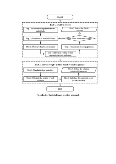
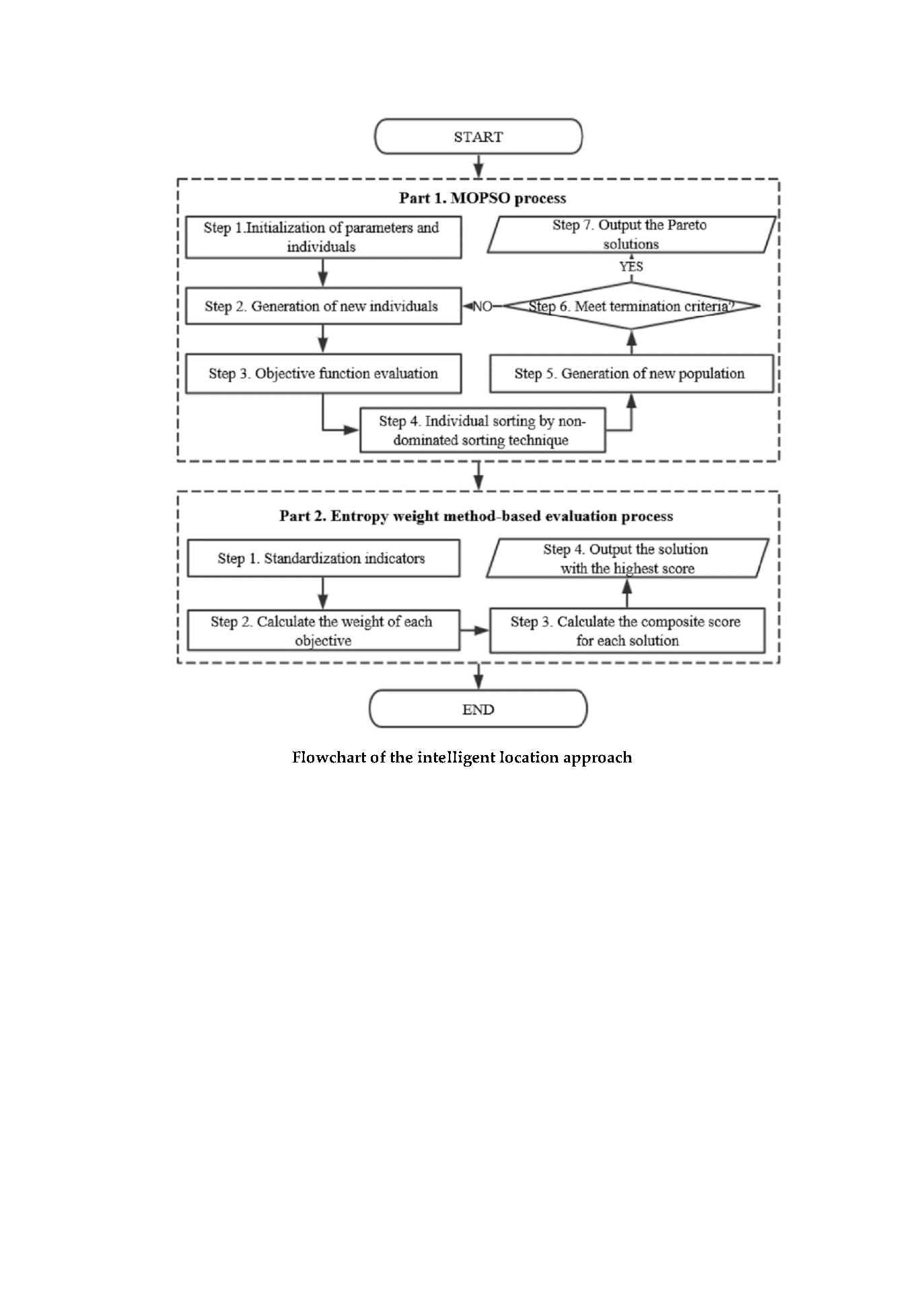
Since the three objectives to be optimized are conflicting, a single optimal solution cannot be found and a multi-objective optimization is needed to find Pareto optimal solutions. Thus, this research proposes an intelligent multi-objective location approach to solve the investigated multi-objective CS location problem based on massive GPS data. This intelligent approach can be divided into two parts: an improved multi-objective particle swarm optimization (MOPSO) process and an entropy weight method-based evaluation process. In the first part, we construct an improved MOPSO process by integrating the discrete particle swarm optimization (PSO) algorithm and the non-dominated sorting technique to produce the Pareto optimal solutions to the investigated problem. This process provides a very efficient procedure in keeping the elitism optimization process as well as preserving the diversity, which assures a good convergence towards the Pareto-optimal front without losing the solution diversity. After obtaining the Pareto optimal solutions, in the second part, we evaluate these solutions and select the one with the highest comprehensive scores based on the entropy weight method [32], which determines the objective weight according to the variability of objective indicators obtained by Pareto optimal solutions’ objective function values and avoids the subjectivity of determining objectives’ weights. The flowchart of this approach is shown in Figure 1.

4.1. Improved MOPSO Process

The improved MOPSO process is employed to generate the Pareto optimal solutions to the investigated problem. The main procedures involved of Part 1 in Figure 1 are described as follows.

4.1.1. Initialization of Parameters and Individuals

Initialization of parameters and individuals are implemented first. The parameters utilized in the optimization process that are initialized include: the population size $N$ = 150, the maximal number of iterations $g_{\max }=80$ and the current iteration count $g=1$. Each individual has a position string and a velocity string. The position string is represented as $\left[y_1,y_2,\dots ,y_I\right]$ to reveals the location plan whereas the velocity string is expressed as $\left[v_1,v_2,\dots ,v_I\right]$ to reflect the moving velocity of the individual, where $I$ is equal to the number of candidate stations. $v_i$ is limited in $\left[-10,10\right]$. The position string and velocity string of each individual are initialized randomly in step 1.

4.1.2. Generation of New Individuals

For each iteration $g$, the $n\mathrm{th}$ individual’s best position $Pbes{t}_n$ in its previous optimization process and the best position $Gbest$ of the population $P_{g-1}$ should be found for updating individuals’ speeds and positions in $P_g$. If the $n\mathrm{th}$ individual’s positions obtained during all previous iterations in its optimization process are non-dominating, then we randomly select one as $Pbes{t}_n$. The best position $Gbest$ of the population $P_{g-1}$ is acquired through non-dominated sorting technique introduced in Section 4.1.4. Then, the speed and position of each bit for all individuals are updated according to the formulas (17)–(19), where $w$ is weight of inertia and equal to 0.8, $c_1,c_2$ are learning factors and $c_1=c_2=2$, the random numbers $r_1=0.6$ and $r_2=0.3$. $rand\left(\right)$ represents a random number uniformly distributed between [0, 1].

$$v_i=w{v}_i+c_1{r}_1\left(Pbes{t}_i-y_i\right)+c_2{r}_2\left(Gbest-y_i\right),\forall i$$

(17)

$$s\left(v_i\right)=\frac{1}{1+\exp \left(-v_i\right)},\forall i$$

(18)

$$y_i=\{\begin{array}{l}1,\mathrm{if}rand\left(\right)\le s\left(v_i\right)\\ 0,\mathrm{otherwise}\end{array},\forall i$$

(19)

Through the process above, new individuals produced and they form the offspring population $Q_g$.

4.1.3. Objective Function Evaluation

Given candidate individual $y$ and trips data extracted from massive GPS trajectory data as inputs, then individual’s objective function values are calculated according to the method below. The value of objective function (1) is the summation of values of elements in the individual. The value of objective function (2) is calculated by formula (2) described in Section 3.2. For any trip, the driver decides whether the PHEV needs to be recharged. If the conditions in constraint (8) are satisfied, the vehicle goes to the CS and is fully recharged; otherwise, the driver starts the next trip without recharging. If there are multiple CSs that meet the conditions, the driver selects the nearest one. The remaining electricity of a trip is related to its previous trips’ electricity consumption and calculated by formulas (4)–(6). During this process, information about charging behaviors such as $t_{jk}$, the index $i$ of this CS, $E_{jk}$ and $C_{ijk}$ are recorded if the $j\mathrm{th}$ vehicle goes to charge after the $k\mathrm{th}$ trip. The value of objective function (2) is calculated when completing all trips of all vehicles successively. Then, based on the charging information obtained when calculating function (2), according to the arrival time of a vehicle and the departure time of the preceding vehicles calculated by formula (7), the total number of vehicles $q_{t_{jk}}^i$ in the $i\mathrm{th}$ CS at that time can be obtained by formulas (12) and (13). In each CS, vehicles queue to recharge by their arrival time, the congestion situation and the waiting time are computed by formula (14). After finishing all trips of all vehicles, objective function (3) is thus solved. The fitness of the $n\mathrm{th}$ individual is represented as $\left\{f_1^n,f_2^n,f_3^n\right\}$ because each individual has three objective values. The lower the three values, the better the fitness.

4.1.4. Individual Sorting by Non-Dominated Sorting Technique

The non-dominated sorting technique proposed in the non-dominated sorting genetic algorithm (NSGA-II) is adopted in sorting candidate individuals, which contains two procedures: fast-non-dominated sorting and calculation of crowding distance. Suppose the parent population is $P_g$, the offspring population $Q_g$ is updated from $P_g$ adopting the method described in Section 4.1.2, and the combined population is $R_g=P_g\cup Q_g$ (size = 2N). $R_g$ is divided into different non-domination levels (F1, F2, etc.) by performing fast-non-dominated sorting procedure. Individuals in the same level do not dominate one another. The higher the non-domination level of the individual, the better the fitness.

Crowding distance calculation procedure is put forward to compare fitness among individuals at the same nondomination level to ensure the results are more evenly distributed in the objective functions space and maintain population diversity. The crowding distance of the $n\mathrm{th}$ individual is the distance between two individuals adjacent to $n$ in the objective functions space. Detailed calculation process can refer to [33].

4.1.5. Generation of Populations

For the initial population $P_1$, the individuals in it are generated randomly based on the representation described in Section 4.1.1. $Pbes{t}_n$ is initialized to the $n\mathrm{th}$ individual itself and $Gbest$ is initialized to a random individual.

For the population $P_{g+1},g\in \left[1,g_{\max }\right]$, the candidate population $S_g$ is constructed by selecting individuals of different nondomination levels layer by layer starting from $F_1$ until $\left|S_g\right|\ge N$. Assume that the last level included is the $F_l$. Individuals in $F_1,F_2,\dots ,F_{l-1}$ have been selected for $P_{g+1}$, then individuals in $F_l$ are picked by prioritizing them with large crowding distances until $\left|P_{g+1}\right|=N$. The new population $P_{g+1}$ are produced. $Gbest$ of population $P_{g+1}$ is the individual with the largest crowding distance in $F_1$ accordingly.

Repeat the above process and increment the iteration count until $g=g_{\max }$. The Pareto optimal solutions are gained eventually.

4.2. Entropy Weight Method-Based Evaluation Process

The entropy weight method-based evaluation process is applied to select the optimal one from the Pareto optimal solutions acquired in Part 1 of the intelligent approach, which is illustrated in Part 2 of Figure 1. Detailed steps are as follows.

4.2.1. Standardization

Suppose there are $n_{opt}$ Pareto optimal location solutions. Indicator $f_{nm}$ is the value of the $m\mathrm{th}$ objective of the $n\mathrm{th}$ Pareto optimal solution. First, $f_{nm}$ needs to be normalized as $f_{nm}^{\prime }$. If the objective function is a positive indicator, its standardization process is in accordance with formula (20); otherwise, it uses formula (21). Due to the three objectives in this research are negative indicators, their standardization applies formula (21).

$$f_{nm}^{\prime }=\frac{f_{nm}-\min \left\{f_{1m},\dots ,f_{n_{opt}m}\right\}}{\max \left\{f_{1m},\dots ,f_{n_{opt}m}\right\}-\min \left\{f_{1m},\dots ,f_{n_{opt}m}\right\}},\forall n\in [1,n_{opt}],m\in [1,2,3]$$

(20)

$$f_{nm}^{\prime }=\frac{\max \left\{f_{1m},\dots ,f_{n_{opt}m}\right\}-f_{nm}}{\max \left\{f_{1m},\dots ,f_{n_{opt}m}\right\}-\min \left\{f_{1m},\dots ,f_{n_{opt}m}\right\}},\forall n\in [1,n_{opt}],m\in [1,2,3]$$

(21)

Then, the proportion of $f_{nm}^{\prime }$ in each objective is calculated by formula (22).

$$p_{nm}=\frac{f_{nm}^{\prime }}{{\displaystyle \sum _{n=1}^{n_{opt}}{f}_{nm}^{\prime }}},\forall n\in [1,n_{opt}],m\in [1,2,3]$$

(22)

4.2.2. Calculation of Objectives’ Weights and Solutions’ Composite Scores

Calculation of each objective’s weight depends on the entropy $e_m$ of each objective and the information entropy redundancy $d_m$ that formulated in Equations (23) and (24). $e_m$ represents the information entropy provided by the $m\mathrm{th}$ objective. The smaller the value of $e_m$, the more information the $m\mathrm{th}$ objective provides in the evaluation process.

$$e_m=-\frac{1}{\ln \left(n_{opt}\right)}{\displaystyle \sum _{n=1}^{n_{opt}}{p}_{nm}\ln (p_{nm})},\forall n\in [1,n_{opt}],m\in [1,2,3]$$

(23)

$$d_m=1-e_m,\forall m\in \left[1,2,3\right]$$

(24)

Then, the weight $w_m$ of each objective is calculated according to formula (25). The smaller the value of $e_m$, the greater the value of $w_m$. Finally, each location solution among the Pareto optimal solutions has a composite score calculated by formula (26) and the location solution with the highest score is the optimal solution to the investigated problem.

$$w_m=\frac{d_m}{{\displaystyle \sum _{m=1}^3{d}_m}},\forall m\in [1,2,3]$$

(25)

$$s_n={\displaystyle \sum _{m=1}^3{w}_m{p}_{nm}},\forall n\in \left[1,n_{opt}\right],m\in \left[1,2,3\right]$$

(26)

5. Numerical Experiments and Discussions

5.1. Data Collection and Processing

To obtain the travel trips of floating vehicles, this research collects and uses the GPS trajectory data of taxis in Chengdu, China. The GPS-enabled device installed in each taxi collects the vehicle’s positions in latitude and longitude, and travel speed in a real-time manner (roughly once per several seconds). One-month data, from 0:00 on 1 June 2015, to 23:59 on 30 June 2015, are collected. These data consist of more than 2 billion original data records, and can reflect the real-time operation statuses of more than 10,000 taxis per day.

The raw trajectory data should be processed to obtain the trips data of each taxi to simulate travel and recharge patterns of PHEVs. In the process procedure, if the parking time of the taxi is not less than 30 min, we think this parking event is the boundary between trips. Parking events with less than 30 min of parking time between any two consecutive trips are neglected and these trips are consolidated to a large trip. Thus, trips data with parking time of not less than 30 min are generated directly from the raw taxi GPS trajectory data. Then, trips data were cleaned by deleting invalid trips caused by data recording or transmission errors and irrational trips with too long (>350 km) or too short (<1 km) distances. Finally, we get the dataset of over 700,000 valid trips in total that stored by vehicle ID and each vehicle’s trips are numbered sequentially by time. The number of vehicles is 10,500, and the time span is 30 days. The data fields of trip records are described in

Table 2. Data fields of trip records.

Data Fields	Description
Vehicle ID	Unique vehicle number.
Trip Number	Unique trip number of a vehicle.
Parking Position	Parking location of a vehicle, expressed in latitude and longitude.
Travel Distance	Length of the current trip, expressed in kilometers.
End Time	End time of current trip.

.

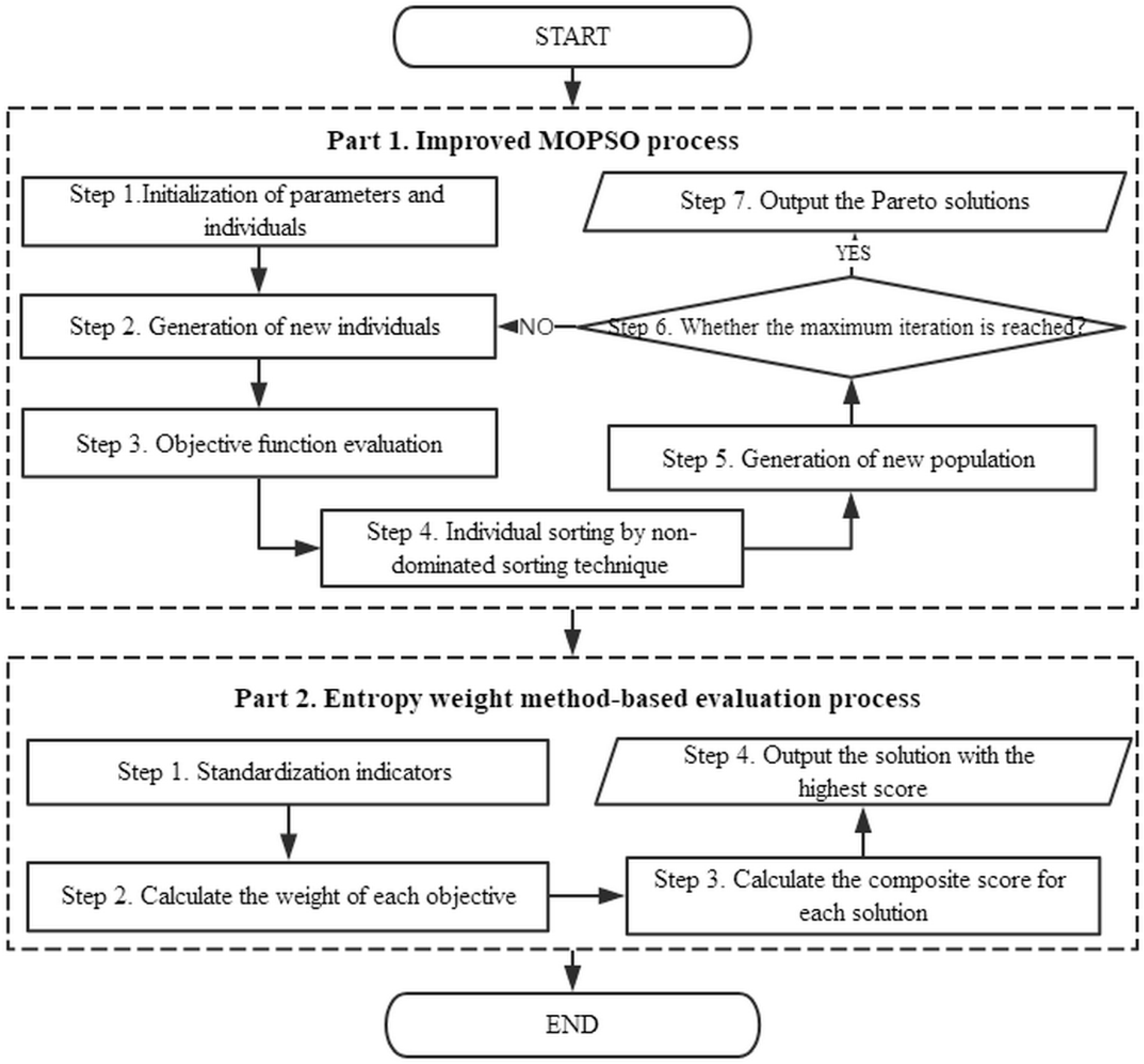
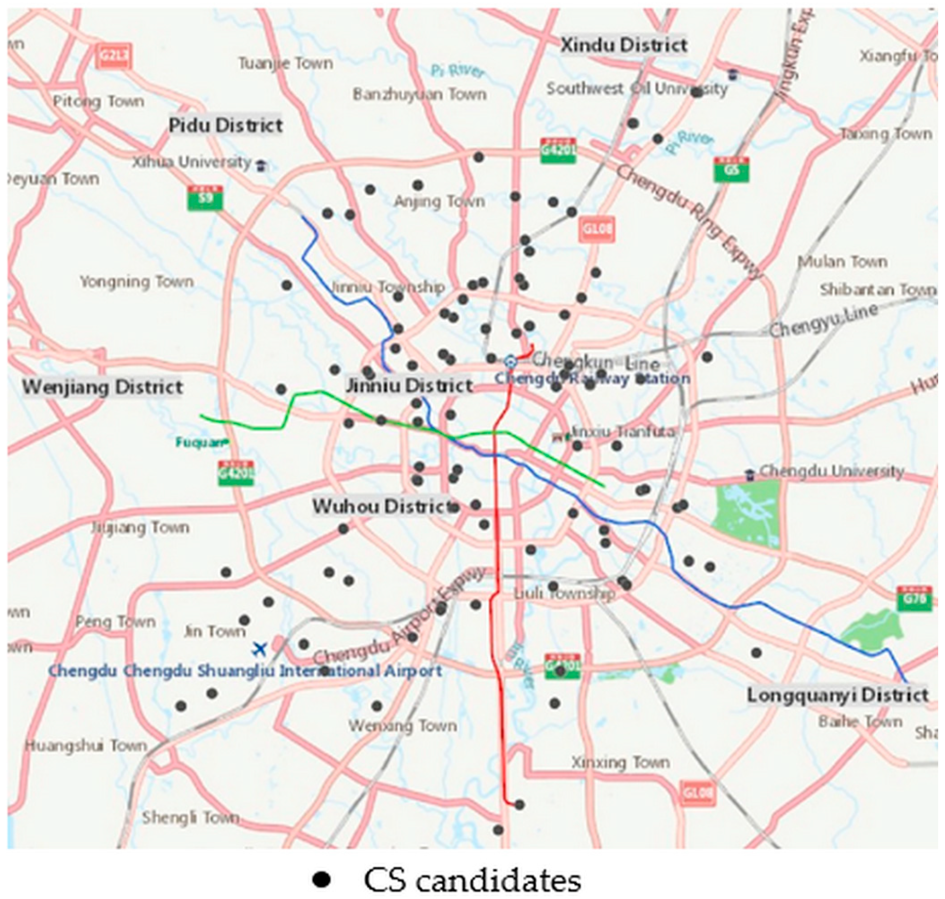
We suppose the end location of the current trip is the start location of the next trip. If there are CSs within a given service radius around the parking position and the remaining capacity is less than $c{E}_j$, drivers will go to charge. Thus, charging demands and charging behaviors are obtained based on travel trips and the deployment of CSs. As for CS candidates, due to the construction of CSs will occupy valuable land resources, especially in the first and second-tier cities, there is no sufficient land to construct them. So, this study selected some existing gasoline stations as candidate sites for CSs. There are more than 300 gasoline stations in Chengdu currently. The top 100 sites from existing gasoline stations were selected, based on the number of parking events occurring around each station because they cover 99% of parking points. Figure 2 shows the distribution of CSs candidates.

Trip-related parameters required for the mathematical model are $d_{jk}$, $d_{ijk}$ and $t_{jk}$. $d_{jk}$ denotes the travel distance described in Table 2. $d_{ijk}$ is the distance from the parking position of the $j\mathrm{th}$ vehicle’s the $k\mathrm{th}$ trip to the $i\mathrm{th}$ CS candidate’s location. $t_{jk}$ represents the time of the $j\mathrm{th}$ vehicle arrives at CS after the $k\mathrm{th}$ trip, but in numerical experiments, $t_{jk}$ is the end time described in Table 2 for simplifying calculations.

Given the location solution $y$ and travel trips of floating vehicles, the values of objective functions can be calculated by the method described in Section 4.1.3.

5.2. Results and Discussions

This section presents the experimental results and discusses the performances of different solutions. The solutions’ performances are evaluated by three indicators corresponding to the three objective functions presented in Section 3.2, including the number of CSs, daily average CO₂ emissions reduction (daily ACER, unit: tons per day) and average waiting time (AWT, unit: hours per trip). The number of CSs and AWT are the values of objective functions (1) and (3). Daily ACER is the CO₂ emissions reduction generated by PHEVs in the case area compared to using gasoline in all trips, which is calculated by formula (27).

$$\mathrm{Daily}\mathrm{ACER}=\frac{({\displaystyle \sum _{j=1}^J\sum _{k=1}^{K_j}{d}_{jk}+\sum _{i=1}^I\sum _{j=1}^J\sum _{k=1}^{K_j}2Z_{ijk}{d}_{ijk}})\gamma -f_2(y_i,D_{ijk})}{30}$$

(27)

5.2.1. Parameter Setting and Charging Station Location Solutions

Parameters listed in Section 3.1 other than trip-related parameters ($d_{jk}$, $d_{ijk}$, $t_{jk}$) need to be set in the proposal approach and experiments.

Some of them are set according to the literature, including $W_a=0.22\mathrm{kWh}/\mathrm{km}$ [16], $\lambda =0.47\mathrm{kg}/\mathrm{kwh}$ [34], ${\gamma }^{\prime }=0.22\mathrm{kg}/\mathrm{km}$ [35]. Some of them are set based on the information provided by Alternative Fuels Data Center (AFDC) of U.S. Department of Energy [36], including $W_b=0.17\mathrm{L}/\mathrm{km}$, $t_0$ = 15 min, $\beta$ = 14 kWh/h, the PHEVs’ fuel consumption per 100 km is 10 L and $\gamma =2.24\mathrm{kg}/\mathrm{L}$, a PHEV can travel nearly 100 miles on electricity alone and $E_j=35\mathrm{kWh}$ is converted based on this information and $W_a$. We set $c=30\%$, $r=2\mathrm{km}$, $s=20$ and $I=100$ according to the realistic requirements of the case city. $M$ is a sufficiently large number and we set $M$ = 100,000.

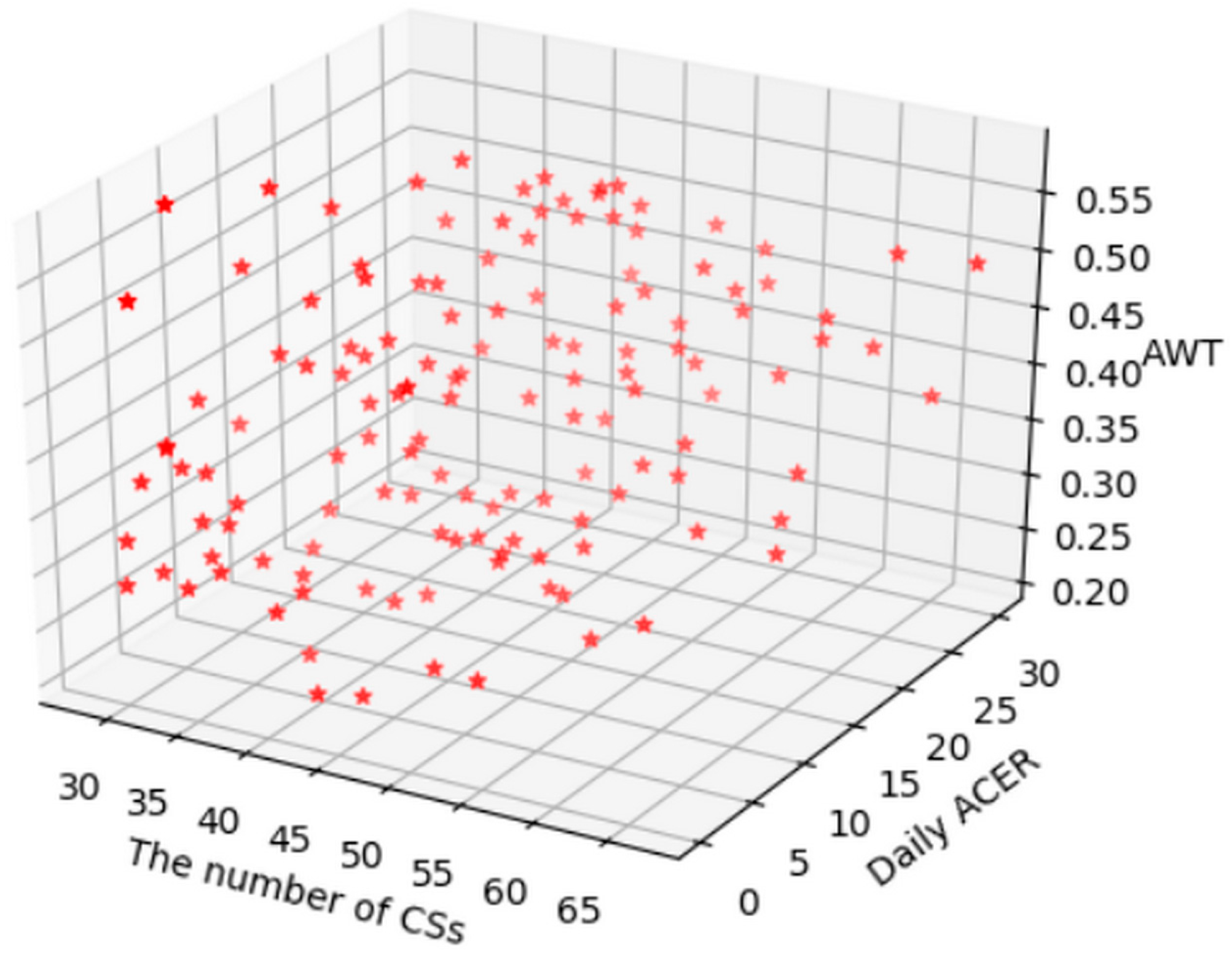
A total of 137 Pareto optimal solutions are obtained by the improved MOPSO process, which is shown in Figure 3.

The descriptive statistics of the objective values generated by these 137 Pareto optimal solutions are described in

Table 3. Descriptive statistics of the Pareto optimal solutions.

Indicators	Min	Median	Mean	Max	Mode	Standard Deviation
The number of CSs	28	42	43	67	40	8.87
Daily ACER (t/d)	0.22	15.65	16.14	30.36	-	7.66
AWT (h/trip)	0.21	0.39	0.39	0.58	-	0.10

. The number of CSs varies from 28 to 67. Daily ACER varies from 0.22 to 30.36 tons per day and the average value is 16.14. AWT varies from 0.21 to 0.58 h and it has the most concentrated distribution.

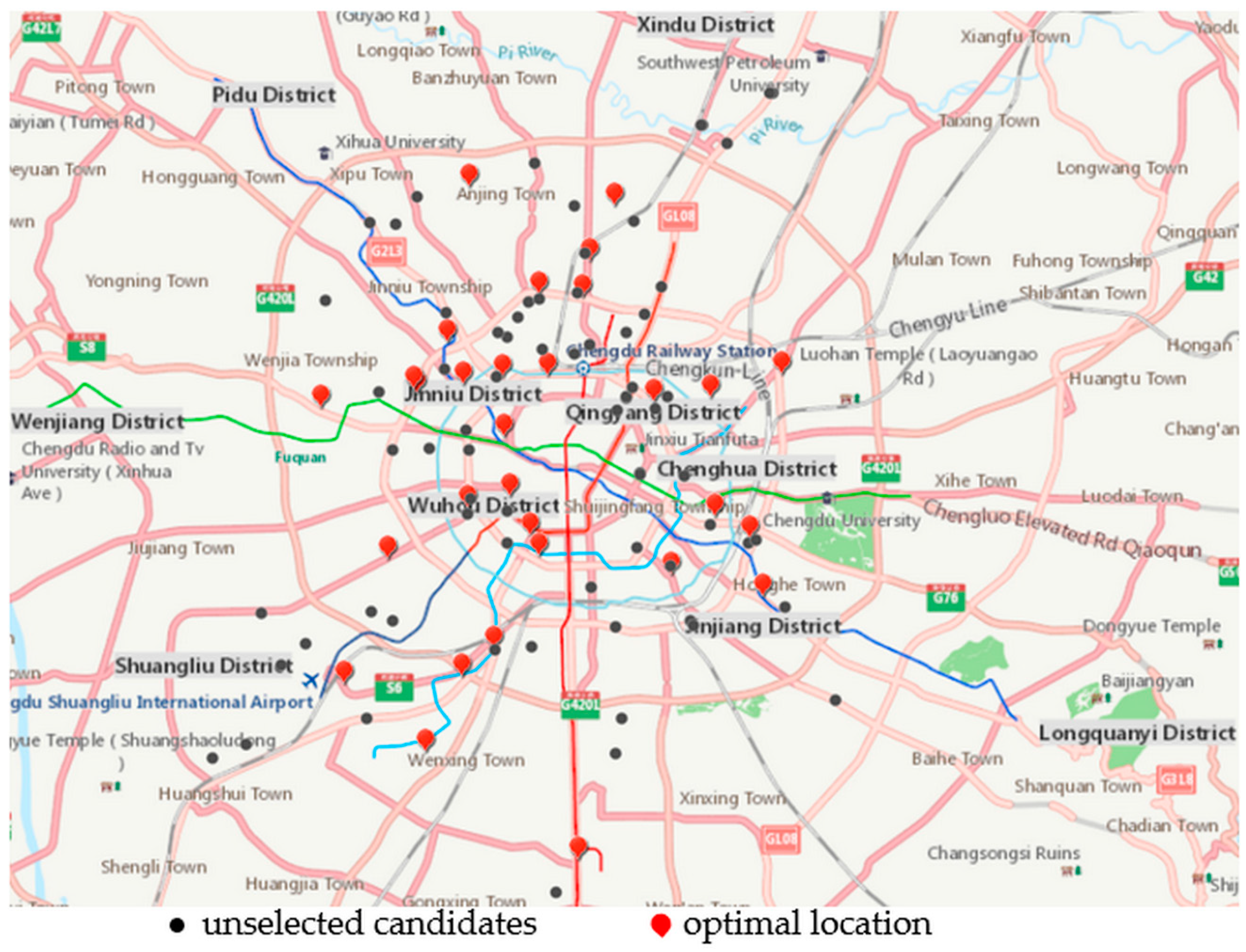
Afterwards, the final optimal solution is selected by the entropy weight method-based evaluation process introduced in Section 4.2. Figure 4 shows the deployment of this solution, in which red points represent locations selected to install CSs and the black points represent the candidate sites not being selected.

Table 4. The performance of optimal location.

Solution	Number of CSs	Daily ACER(t/d)	AWT(h/trip)
Optimal location	30	10.39	0.37

reveals the performance of this location solution, which leads to a total of 30 CSs, 10.39 tons of daily ACER that require at least 10 hectares of forests to absorb within one day [37] and 0.37 h (22.2 min) of AWT for trips that need to be recharged.

To verify the reliability of the results obtained by our model, the effects of different parameters on location results and the performance comparison of single-objective and multi-objective models are presented in Section 5.2.2 and Section 5.2.3.

5.2.2. Effects of Different Parameters on Location Results

Table 5. Comparison of location performances generated by different parameters.

Different Parameters		The Number of CSs	Daily ACER (t/d)	AWT (h/trip)
Charging threshold	$c=10\%$	31	3.31	0.23
	$c=30\%$	30	10.39	0.37
	$c=50\%$	29	22.36	0.65
The number of chargers in each CS	$s=10$	29	8.74	1.72
	$s=20$	30	10.39	0.37
	$s=30$	30	16.94	0.29
Service radius of CSs	$r=1$	52	0.51	0.04
	$r=2$	30	10.39	0.37
	$r=3$	26	29.74	1.76

shows the location performances generated by different settings of parameters $c$, $s$ and $r$.

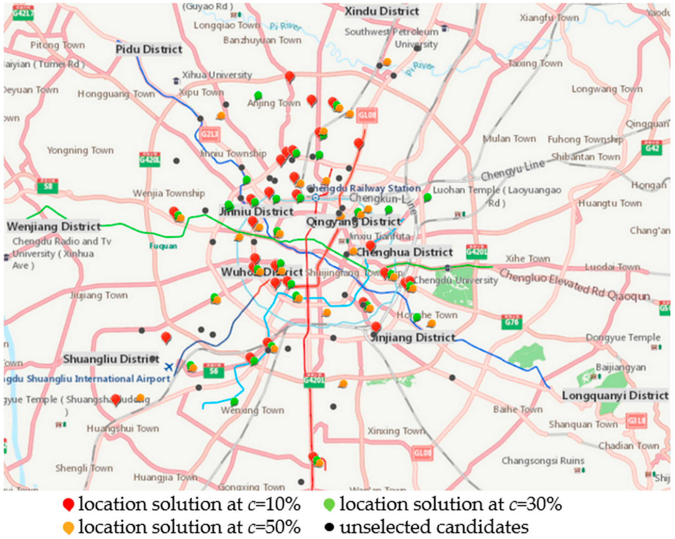
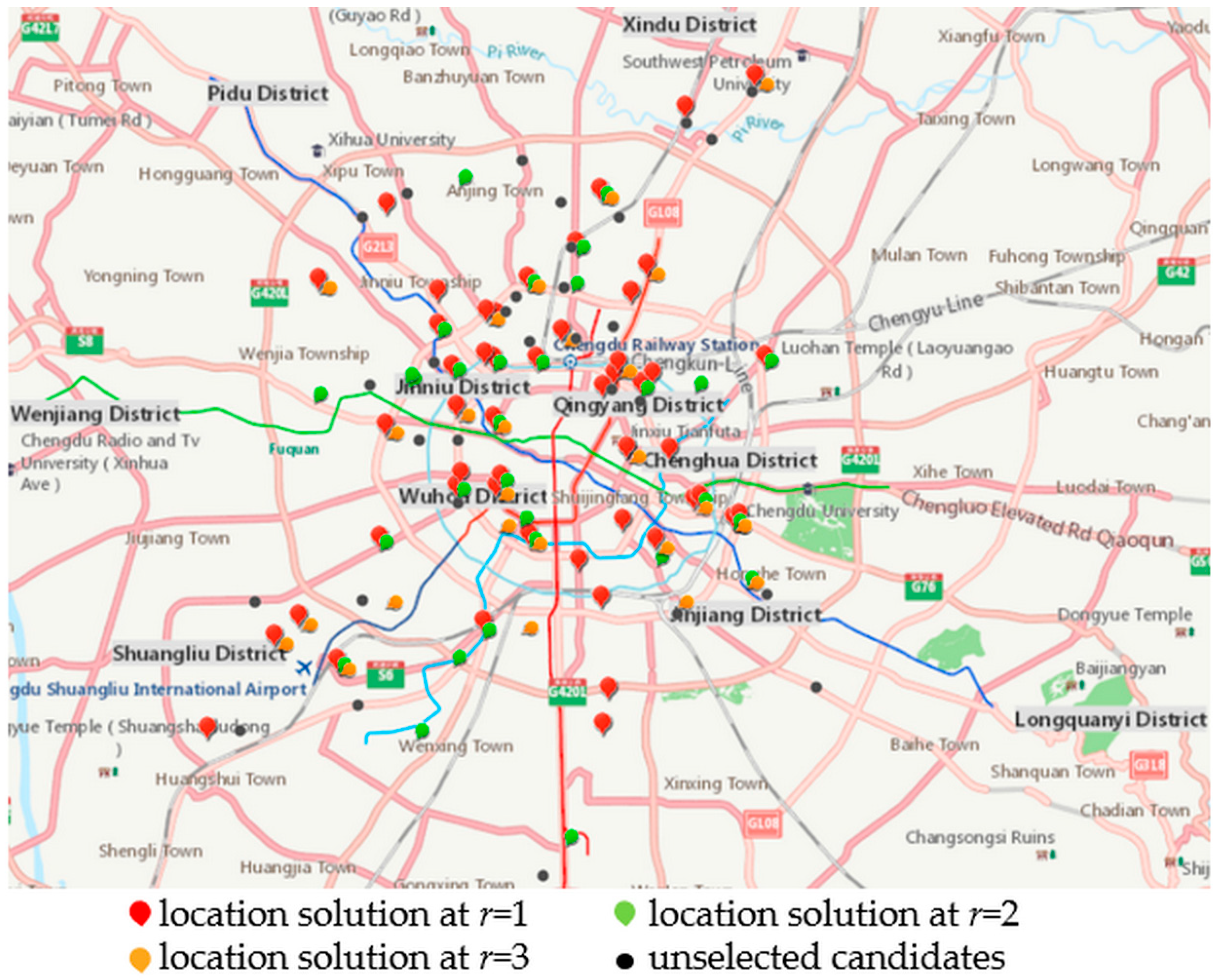
As seen in this table, the charging threshold $c$ has relatively few effects on the number of CSs, but affect significantly the other two indicators. Drivers’ charging behaviors tend to be conservative with the increases of $c$ and they are even more reluctant to withstand the inconvenience caused by the exhaustion of electricity. The number of trips that need to be recharged also increases. Therefore, with the increases of $c$, the possibility of completing the trip by gasoline decreases and the values of daily ACER and AWT increase. Thus, questionnaires can be utilized to investigate the charging attitudes of drivers in Chengdu and $c$ can be set according to their charging behavioral preferences. The CS placements at different $c$ are illustrated in Figure 5. The location solutions at $c=10\%$, $c=30\%$ and $c=50\%$ are represented by red, green and yellow points respectively. Unselected candidate stations are represented by black points. When drivers’ charging preferences cannot be judged by decision makers, $c$ can be set as 30%.

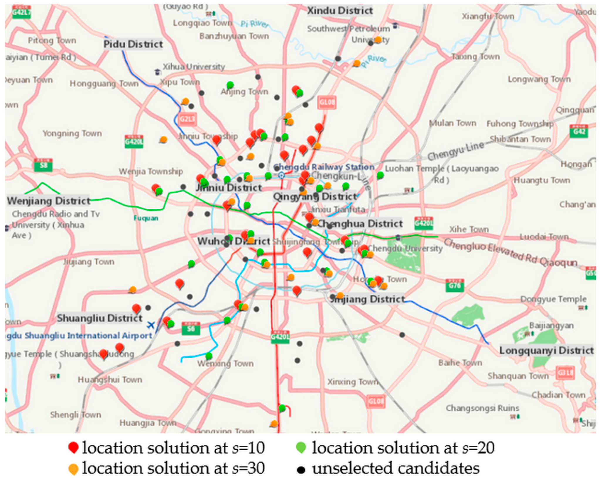
Same as $c$, the number of chargers $s$ at each CS has few effects on the number of CSs but has significant effects on the other indicators. With the increase of $s$ under the case of a similar number of CSs, the number of vehicles that are allowed to charge at the same time evidently increases and the city’s overall charging service capacity improves. Thus, daily ACER increases and AWT decreases. Under the same conditions, the performance of the solution becomes better as $s$ increases but it is limited by land resources in reality. Figure 6 shows the CSs locations of different $s$. The location at $s=10,20\mathrm{and}30$ are consisted by red, green and yellow points, black points represent the remaining unselected candidate stations.

Service radius $r$ of CSs has significant influence on all indicators. With the increases of $r$, the number of CSs decreases, daily ACER and AWT increase. As $r$ increases, the service range of a CS expands, thus the charging demands that cannot be satisfied because of the service radius originally are satisfied and trips required to complete using gasoline are reduced, but the number of vehicles to be recharged in the CS increases and the queue time increases when $s$ unchanged. An increase in $r$ will result in a sparse distribution of CSs, which affects drivers’ charging behaviors negatively. So, $r$ preferably does not exceed 2 km in reality. The location solutions at different $r$ are illustrated in Figure 7, in which the location at $r=1,2\mathrm{and}3$ are represented by red, green and yellow points. Unselected candidate stations are represented by black points.

5.2.3. Performance Comparison of Single-Objective and Multi-Objective Models

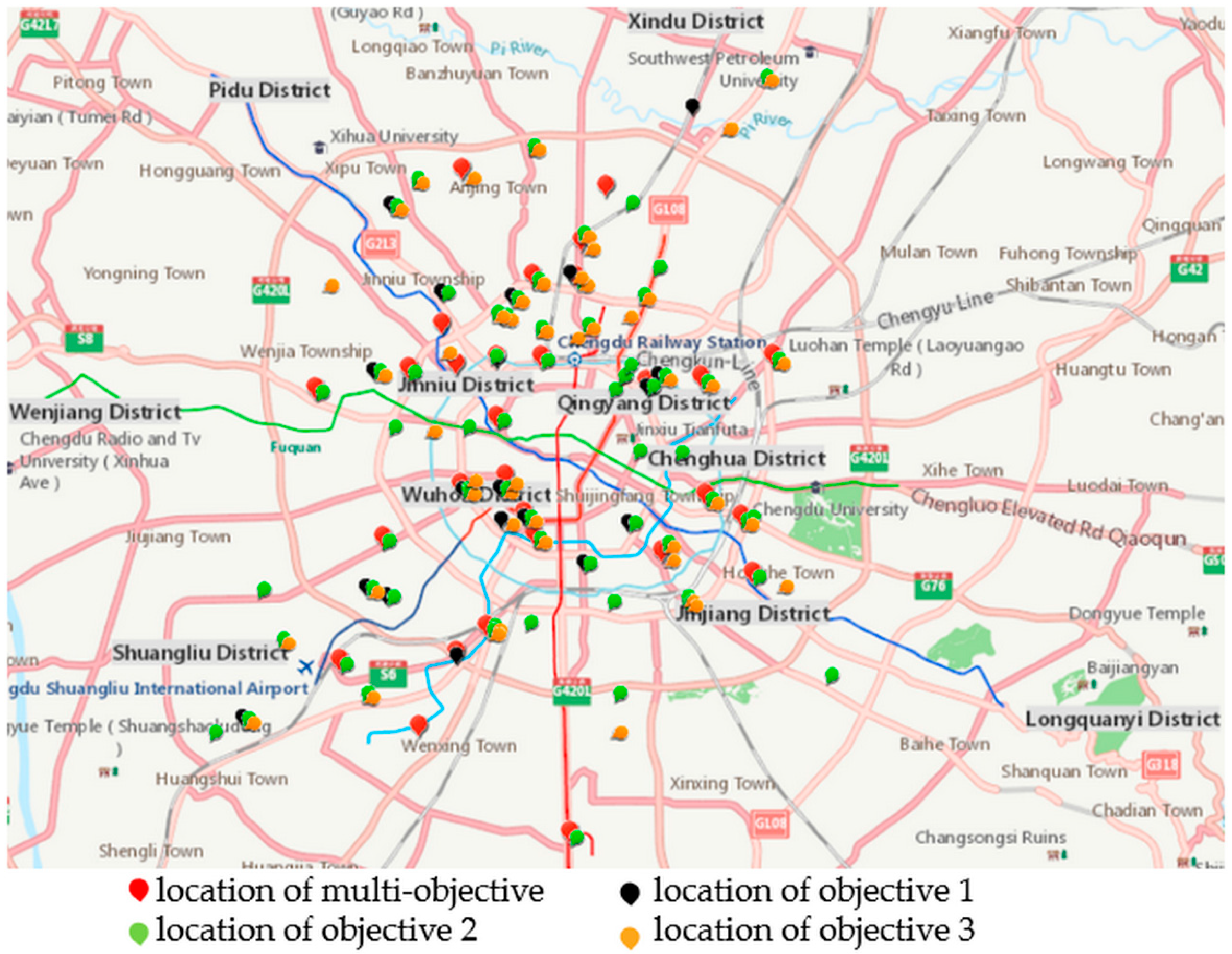
This section discusses the performance differences generated by single-objective and multi-objective CS location models, to address the necessity of considering multiple objectives in CS location problems. The comparison results are shown in

Table 6. Performance comparison of different models.

Different Models	The Number of CSs	Daily ACER (t/d)	AWT (h/trip)
Three objectives	30	10.39	0.37
Objective 1	20	0.67	0.47
Objective 2	66	30.82	0.42
Objective 3	47	4.98	0.19

, in which the first row shows the results generated by the model with the consideration of three objectives, the second to the fourth rows show the results generated by the models with objectiv1 to objective 3 respectively.

Table 6 shows that each single-objective model can generate the optimal value of its corresponding objective function, but the performances of other two indicators are not so good. The locations of objective 1 and objective 2 have the maximal and minimal number of CSs respectively. But their values of AWT are almost equal. The solution caused by objective 3 has the best performance in terms of AWT but the performances of other indicators are not obviously superior. In general, the performance of the three objectives model is more reliable and practical, the values of its indicators are slightly lower than the value of the corresponding single-objective model and higher than the values of other two models. Consequently, applying three-objectives model is the most reliable choice when planner is unable to determine the weights of different objectives. The locations of CSs generated by different models are illustrated in Figure 8, in which the location of multi-objective model is represented by red points, and the locations of objectives 1, 2 and 3 are represented by black, green and yellow points.

6. Conclusions

This paper presented a multi-objective model for public charging station location problem considering the triple bottom line principle under the trend of sustainable development. The mathematical model has been established with three sustainable objectives, including minimizing the number of CSs, minimizing the total CO₂ emissions, and minimizing the average waiting time of trips that need to be recharged, which are especially beneficial for local governments to achieve sustainable development goals.

An intelligent multi-objective location approach is developed to tackle the investigated problem. In this approach, an improved MOPSO process, combining a discrete PSO algorithm with a non-dominated sorting technique, is proposed to seek a set of Pareto optimal solutions, and an entropy weight method-based evaluation process is put forward to pick out the final preferred solution from the set of Pareto optimal solutions. The efficiency of the proposed multi-objective model has been validated by employing a large number of real trips data of floating vehicles. Experimental comparisons were conducted to examine the impacts of three parameters (charging threshold, the number of chargers and service radius of CSs) on location results and the necessity of the proposed multi-objective model.

This research assumes that all CSs have the same capacity. Our further research will consider the location problem of CSs with different capacities. Comparing the performance of the improved MOPSO process proposed in this paper with other existing multi-objective evolutionary optimization algorithms is another future direction worthy to do.

References

- Guo, Z.X.; Zhang, D.Q.; Liu, H.T.; He, Z.G.; Shi, L.Y. Green transportation scheduling with pickup time and transport mode selections using a novel multi-objective memetic optimization approach. Transp. Res. Part D Transp. Environ. 2018, 60, 137–152. [Google Scholar] [CrossRef]
- Bjerkan, K.Y.; Norbech, T.E.; Nordtomme, M.E. Incentives for promoting Battery Electric Vehicle (BEV) adoption in Norway. Transp. Res. Part D Transp. Environ. 2016, 43, 169–180. [Google Scholar] [CrossRef]
- Yuan, C.W.; Wu, D.Y.; Liu, H.C. Using Grey Relational Analysis to Evaluate Energy Consumption, CO2 Emissions and Growth Patterns in China’s Provincial Transportation Sectors. Int. J. Environ. Res. Public Health 2017, 14, 1536. [Google Scholar] [CrossRef] [PubMed]
- He, Z.; Chen, P.; Liu, H.; Guo, Z. Performance measurement system and strategies for developing low-carbon logistics: A case study in China. J. Clean. Prod. 2017, 156, 395–405. [Google Scholar] [CrossRef]
- Shahrina, N.; Imran, R.; Vasant, P.; Noor, M.A. An Overview of Electric Vehicle Technology a Vision towards Sustainable Transportation; IGI Global: Hershey, PA, USA, 2017; pp. 198–220. [Google Scholar]
- Plotz, P.; Funke, S.A.; Jochem, P. Empirical Fuel Consumption and CO2 Emissions of Plug-In Hybrid Electric Vehicles. J. Ind. Ecol. 2018, 22, 773–784. [Google Scholar] [CrossRef]
- AFDC Electric Vehicle Benefits and Considerations. Available online: https://www.afdc.energy.gov/fuels/electricity_benefits.html (accessed on 16 September 2018).
- Tamayao, M.A.M.; Michalek, J.J.; Hendrickson, C.; Azevedo, I.M.L. Regional Variability and Uncertainty of Electric Vehicle Life Cycle CO2 Emissions across the United States. Environ. Sci. Technol. 2015, 49, 8844–8855. [Google Scholar] [CrossRef] [PubMed]
- Efthymiou, D.; Chrysostomou, K.; Morfoulaki, M.; Aifantopoulou, G. Electric vehicles charging infrastructure location: A genetic algorithm approach. Eur. Transp. Res. Rev. 2017, 9, 27. [Google Scholar] [CrossRef]
- Wang, C.J.; Liu, Q.; Guo, Z. Green Project Planning with Realistic Multi-Objective Consideration in Developing Sustainable Port. Sustainability 2018, 10, 2385. [Google Scholar] [CrossRef]
- Guo, Z.X.; Liu, H.T.; Zhang, D.Q.; Yang, J. Green Supplier Evaluation and Selection in Apparel Manufacturing Using a Fuzzy Multi-Criteria Decision-Making Approach. Sustainability 2017, 9, 650. [Google Scholar]
- Bhattacharya, U.; Rao, J.R.; Tiwari, R.N. Fuzzy multi-criteria facility location problem. Fuzzy Sets Syst. 1992, 51, 277–287. [Google Scholar] [CrossRef]
- Vancamp, D.J.; Carter, M.W.; Vannelli, A. A Nonlinear Optimization Approach for Solving Facility Layout Problems. Eur. J. Oper. Res. 1992, 57, 174–189. [Google Scholar] [CrossRef]
- Snyder, L.V. Facility location under uncertainty: A review. IIE Trans. 2006, 38, 547–564. [Google Scholar] [CrossRef]
- Dong, J.; Liu, C.Z.; Lin, Z.H. Charging infrastructure planning for promoting battery electric vehicles: An activity-based approach using multiday travel data. Transp. Res. Part C Emerg. Technol. 2014, 38, 44–55. [Google Scholar] [CrossRef]
- Shahraki, N.; Cai, H.; Turkay, M.; Xu, M. Optimal locations of electric public charging stations using real world vehicle travel patterns. Transp. Res. Part D Transp. Environ. 2015, 41, 165–176. [Google Scholar] [CrossRef] [Green Version]
- He, F.; Yin, Y.; Zhou, J. Deploying public charging stations for electric vehicles on urban road networks. Transp. Res. Part C Emerg. Technol. 2015, 60, 227–240. [Google Scholar] [CrossRef]
- Li, S.; Huang, Y.; Mason, S.J. A multi-period optimization model for the deployment of public electric vehicle charging stations on network. Transp. Res. Part C Emerg. Technol. 2016, 65, 128–143. [Google Scholar] [CrossRef]
- Yang, J.; Dong, J.; Hu, L. A data-driven optimization-based approach for siting and sizing of electric taxi charging stations. Transp. Res. Part C Emerg. Technol. 2017, 77, 462–477. [Google Scholar] [CrossRef]
- Tu, W.; Li, Q.; Fang, Z.; Shaw, S.-L.; Zhou, B.; Chang, X. Optimizing the locations of electric taxi charging stations: A spatial–temporal demand coverage approach. Transp. Res. Part C Emerg. Technol. 2016, 65, 172–189. [Google Scholar] [CrossRef] [Green Version]
- He, J.; Yang, H.; Tang, T.Q.; Huang, H.J. An optimal charging station location model with the consideration of electric vehicle’s driving range. Transp. Res. Part C Emerg. Technol. 2018, 86, 641–654. [Google Scholar] [CrossRef]
- Wang, Y.W.; Wang, C.R. Locating passenger vehicle refueling stations. Transp. Res. E 2010, 46, 791–801. [Google Scholar] [CrossRef]
- Yao, W.F.; Zhao, J.H.; Wen, F.S.; Dong, Z.Y.; Xue, Y.S.; Xu, Y.; Meng, K. A Multi-Objective Collaborative Planning Strategy for Integrated Power Distribution and Electric Vehicle Charging Systems. IEEE Trans. Power Syst. 2014, 29, 1811–1821. [Google Scholar] [CrossRef]
- Shinde, P.; Swarup, K.S. A Multiobjective Approach for Optimal Allocation of Charging Station to Electric Vehicles. In Proceedings of the IEEE Annual InIndia Conference, Chennai, India, 16–18 December 2016. [Google Scholar]
- Zhang, S.; Zhu, J.; Wang, B.; Wang, C. Multi-objective Optimization Charging Strategy for Plug-in Electric Vehicles Based on Dynamic Time-of-use Price. Power Syst. Prot. Control 2017, 1, 1–7. [Google Scholar]
- Junhong, L.; Zheyong, Q.; Jiachen, Y.; Chen, G. Urban charging station location model based on multi-objective programming. J. Phys. 2018, 1053, 012028. [Google Scholar]
- Wang, G.; Xu, Z.; Wen, F.; Wong, K.P. Traffic-constrained multi objective Planning of Electric-Vehicle Charging Stations. Trans. Power Deliv. 2013, 28, 2363–2372. [Google Scholar] [CrossRef]
- Zhang, A.P.; Kang, J.E.; Kwon, C. Incorporating demand dynamics in multi-period capacitated fast-charging location planning for electric vehicles. Transp. Res. B 2017, 103, 5–29. [Google Scholar] [CrossRef]
- Spieker, H.; Hagg, A.; Gaier, A.; Meilinger, S.; Asteroth, A. Multi-stage evolution of single- and multi-objective MCLP. Soft Comput. 2017, 21, 4859–4872. [Google Scholar] [CrossRef]
- Xu, M.; Meng, Q.; Liu, K.; Yamamoto, T. Joint charging mode and location choice model for battery electric vehicle users. Transp. Res. B 2017, 103, 68–86. [Google Scholar] [CrossRef]
- Luo, X.; Dong, L.; Dou, Y.; Zhang, N.; Ren, J.Z.; Li, Y.; Sun, L.; Yao, S.Y. Analysis on spatial-temporal features of taxis’ emissions from big data informed travel patterns: A case of Shanghai, China. J. Clean. Prod. 2017, 142, 926–935. [Google Scholar] [CrossRef]
- Wen, L.C.; Zhang, X.F.; Zhu, L.M. Method of ameliorative multi-objective synthetic evaluation based on entropy weight and its application. In Proceedings of the China Control and Decision Conference, Guilin, China, 17–19 June 2009; pp. 1593–1596. [Google Scholar]
- Deb, K.; Pratap, A.; Agarwal, S.; Meyarivan, T. A fast and elitist multiobjective genetic algorithm: NSGA-II. IEEE Trans. Evol. Comput. 2002, 6, 182–197. [Google Scholar] [CrossRef] [Green Version]
- Cai, W.; Wang, C.; Wang, K.; Zhang, Y.; Chen, J. Scenario analysis on CO2 emissions reduction potential in China’s electricity sector. Energy Policy 2007, 35, 6445–6456. [Google Scholar] [CrossRef]
- Huo, H.; Zhang, Q.; Wang, M.Q.; Streets, D.G.; He, K. Environmental Implication of Electric Vehicles in China. Environ. Sci. Technol. 2010, 44, 4856–4861. [Google Scholar] [CrossRef] [PubMed]
- AFDC Alternative Fuels Data Center. Available online: https://www.afdc.energy.gov/ (accessed on 10 January 2018).
- Sicirec Forest and Carbon Capture. Available online: http://www.sicirec.org/definitions/carbon-capture (accessed on 23 June 2018).
Figure 1.
Flowchart of the proposed location approach.
Figure 2.
Distribution of charging station (CS) candidates in Chengdu.
Figure 3.
Pareto-optimal solutions in three-dimensional space.
Figure 4.
Optimal location of CSs.
Figure 5.
The deployments generated by different .
Figure 6.
Figure 7.
Figure 8.
The locations of single-objective and multi-objective models.