Minimization of Logistics Cost and Carbon Emissions Based on Quantum Particle Swarm Optimization

Abstract

This paper aims to simultaneously minimize logistics costs and carbon emissions. For this purpose, a mathematical model for a three-echelon supply chain network is created considering the relevant constraints such as capacity, production cost, transport cost, carbon emissions, and time window, which will be solved by the proposed quantum-particle swarm optimization algorithm. The three-echelon supply chain, consisting of suppliers, distribution centers, and retailers, is established based on the number and location of suppliers, the transport method from suppliers to distribution centers, and the quantity of products to be transported from suppliers to distribution centers and from these centers to retailers. Then, a quantum-particle swarm optimization is described as its performance is validated with different benchmark functions. The scenario analysis validates the model and evaluates its performance to balance the economic benefit and environmental effect.

1. Introduction

The operations in supply chain and logistics are vital tools for businesses to remain competitive in today’s important economic activities. Transportation activities are significant sources of air pollution and greenhouse gas emissions, with the former known to have harmful effects on human health and the latter being responsible for global warming. These issues have raised concerns on reducing the amount of emissions worldwide [1].

As today, the success measures for the companies are considered to be lower costs, lower emissions, shorter production time, shorter lead time, less stock, larger product range, more reliable delivery time, better customer services, higher quality, and providing the efficient coordination between demand, supply, and production; however, the trade-off between cost investment and service levels may change over time. Some leading companies are now proactively implementing “green” initiatives. They are also trying to enhance their supply chain management capability to tackle environmental concerns by focusing more on selecting appropriate facility locations and technologies. We are motivated to study a green supply chain network design problem where an initial investment on environmental protection equipment or techniques should be determined in the design phase. This investment can influence the environmental indicators in the operations phase. Therefore, a trade-off exists between the initial investment and its long-term benefit to environment. With such a concern, decisions regarding facility location and capacity allocation have to be integrated with the decisions regarding environmental investment.

In recent years, there have been many studies solving the optimization problems of supply chain and logistics that are related to design and operation. This research proposes an integrated supply model of first-mile/last-mile delivery [2]. The author describes a real-time scheduling optimization model focusing on the energy efficiency of the operation, and introduces a mathematical model of last-mile delivery problems including scheduling and assignment problems [3]. Varamath proposed modeling and optimization a three-echelon supply chain network using the particle swarm optimization to address the demand uncertainty and constraints posed by every echelon in the supply chain design operations [4]. The measurement of supply chain and logistics solutions is performed allowing the quantification of availability, flexibility, efficiency, and plasticity indicators [5]. Studies show that unmanned aerial vehicles have the potential effectiveness to reduce CO₂ emissions compared to conventional transportation solutions [6]. Researchers have considered three critical environmental issues, namely the energy used in production processes, greenhouse gas (GHG) emissions from production, and transportation activities, and then presented two models (classical and Vendor Managed Inventory coordination) for a two-level closed-loop supply chain [7]. Facing the competitive global market, manufacturers are increasingly dependent on the supply chain network. As one of the strategies of the supply chain, just-in-time greatly reduces the inventory in the workflow through frequent production, which enhances the production efficiency of the enterprise [8]. However, frequent small-scale production requires better responsiveness to transport demands, leading to severe environmental pollution and high transport cost. Based on the just-in-time system [9], Hashem proposed a multi-criterion decision model to optimize the production, quality, price, cost, equipment, and technology of products, and verified that, with this model, both operation and delivery met consumer demand and export quality standard [10]. A just-in-time decision system was put forward that improves the sales, design, and production of the products of the company [11]. To ensure delivery punctuality, Reference [12] Pedro developed a multi-objective mathematical model based on the three-level distribution network, but the modeling process failed to consider the environmental impact. In recent years, the concept of greenness has been introduced to supply chain management to reflect the environmental impact on the management process [12]. The logistics directly bear on the sources of environmental pollution such as greenhouse gas emissions. Despite the growing awareness of green logistics, the environmental constraints are seldom adopted for actual logistics operations. The multi-target fuzzy technique is the most desirable tool to build up a green supply chain network. In general, the multi-target fuzzy models have two conflicting goals, namely, minimal cost and minimal environmental impact. TakingtheCO₂ equivalent as the indicator of the environmental impact of logistics operations, an optimized closed-loop supply chain network was present, which integrated the forward and reverse propagations. Since the classic production and distribution models often pursued minimal cost, it is necessary to create a new combinatory optimization model based on the objectives and constraints of green logistics [13].

In light of the above, this paper aims to minimize the logistics cost and carbon emissions simultaneously. For this purpose, a mathematical model for a three-echelon supply chain network was created considering the relevant constraints such as capacity, production cost, transport cost, carbon emissions, and time window, which are to be solved by the quantum-particle swarm optimization algorithm. The three-echelon supply chain, consisting of suppliers, distribution centers, and retailers, was established based on the number and location of suppliers, the transport method from suppliers to distribution centers, and the quantity of products to be transported from suppliers to distribution centers and then to retailers. Then, the proposed model was applied to a real case of logistics distribution. The results show that the supplier will opt for vehicles with low carbon emissions with the increase in the replenishment time, distances between members of the supply chain, the rate of carbon tax, and the number of retailers.

2. Problem Definition and Modeling

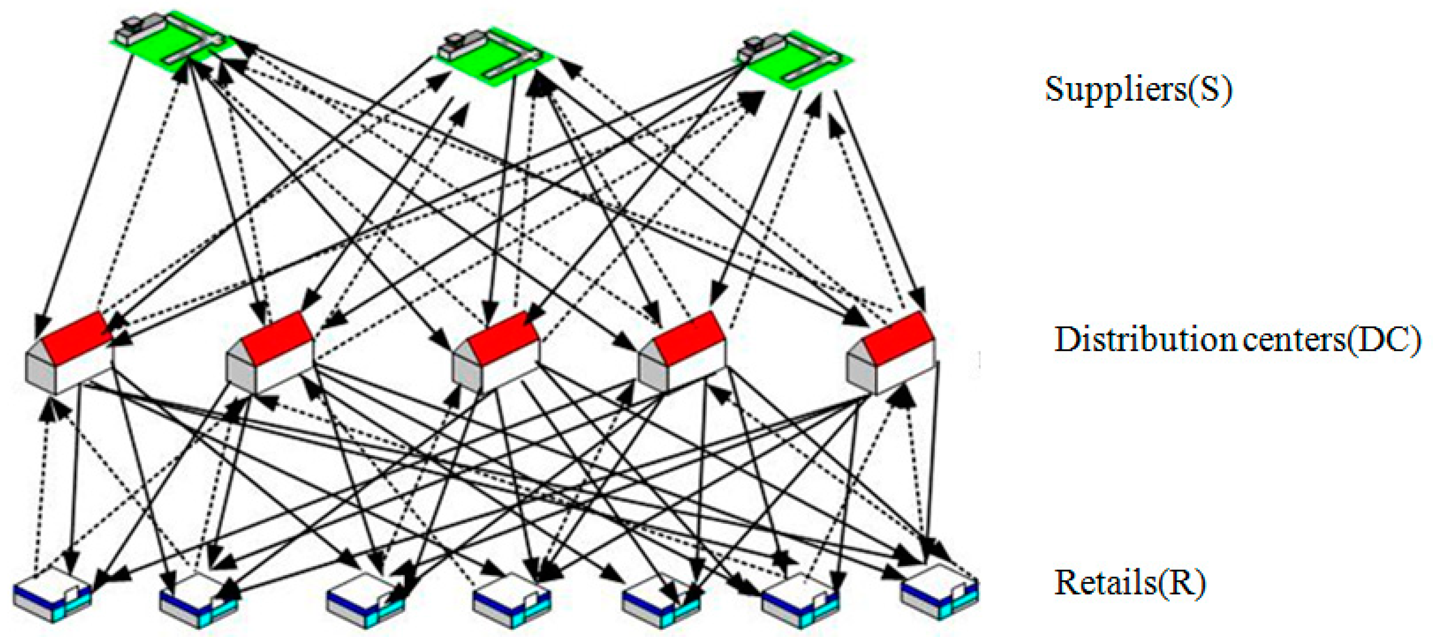
As shown in Figure 1, the three-echelon supply chain network involves suppliers (S), distribution centers (DC), and retailers (R). Let S = 1, 2, …, n be the set of suppliers, j = 1, 2, …, n be the set of distribution centers, and I = 1,2, …, n be the set of retailers. The suppliers, which differ in capacity, need to distribute products to the retailers through the distribution centers. Both environmental and economic factors should be taken into account before making scientific decisions on the route, order quantity, locations, and number of distribution centers of the delivery process [14]. The following hypotheses were put forward:

(1)

The location and capacity of each supplier is fixed. Suitable distribution centers should be selected from multiple potential distribution centers, and the demand for the suitable ones obeys random distribution.

(2)

The carbon emissions in the supply chain network originate from the routes between the suppliers, distribution centers, and retailers (S–DC–R), the site of distribution centers and the inventory of retailers.

(3)

The carbon emissions are measured by the amount of CO₂ release.

(4)

The demand for distribution centers and retailers should be met by the same vehicle; only one vehicle is allowed on each distribution route; all of the vehicles share the same maximum load capacity; each vehicle should return to the distribution center after completing the distribution task.

(5)

Each retailer can be supplied by multiple distribution centers.

(6)

Each distribution center can be supplied by multiple suppliers.

Parameters are as follows:

$S$	represents a collection of factories
$J$	represents the collection of distribution lefts
$I$	represents the set of distributors
$V$	collection of transport vehicles
$u_i$	annual demand of distributor I
$Q_j$	order quantity of the distribution left j each time
$N_i$	distributor I order quantity every time
$w_j$	distribution left j unit product inventory holding cost
$\alpha$	the probability of being out of stock, $1-\alpha$ being the corresponding service level
$Z_{\alpha }$	safety inventory coefficient
$L$	advance order
$u_j$	average demand in the distributor’s j cycle
${\sigma }_j$	the standard deviation in the distributor’s j cycle
$d_{sj}$	$s\in S,j\in J$, the transport distance of factory s to DCj
$d_{ei}$	$\forall \mathrm{e}\in (\mathrm{I}\cup \mathrm{J}),\mathrm{i}\in \mathrm{I}$, the transport distance of node e to node I
${\mathrm{c}}_{sj}$	unit transportation cost of factory s to DCj
$h_{ji}$	unit distribution cost of DCj distribution unit products to Ri
$g_j$	the fixed cost of establishing a potential distribution left
$C_{\max }$	supply chain carbon emission quota
$\theta$	carbon emission limit penalty factor

Decision variables:

$x_{sj}$	represents the number of products shipped from factory s to the potential distribution center
$y_{ji}$	represents the number of products delivered to distributor I by the potential distribution center
$\theta$	represents the carbon emission limit penalty factor

Decision variables:

$$U_j^n{}_{}\{\begin{array}{l}{1}_{}^{}\mathrm{if}\mathrm{DC}j\mathrm{is}\mathrm{open}\\ 0_{}^{}\mathrm{if}\mathrm{otherwise}\end{array}j\in J$$

$$R_{ji}^{}\{\begin{array}{l}{1}_{}^{}\mathrm{if}Ri\mathrm{is}\mathrm{open}\\ 0_{}^{}\mathrm{if}\mathrm{otherwise}\end{array}i\in I$$

$$q_{eiv}^{}{\{\begin{array}{l}{1}_{}^{}{}_{}^{}\mathrm{if}\mathrm{vehicle}v\mathrm{from}\mathrm{node}e\mathrm{to}\mathrm{node}i\\ 0_{}^{}{}_{}^{}\mathrm{if}\mathrm{otherwise}\end{array}}_{}^{}\forall e\in (I\cup J),i\in I$$

(1) Calculate the cost of location–route–inventory [10,11].

The fixed construction cost of distribution center location:

$$M_{DC}={\displaystyle \sum _{j\in J}^{}{\displaystyle \sum _{n\in N_j}^{}{f}_{{}_j}^n}{U}_j^n}$$

(1)

where $f_{{}_j}^n$ is the location cost of distribution center with capacity n.

Transportation cost:

$$M_R={\displaystyle \sum _{s\in S}^{}{\displaystyle \sum _{j\in J}^{}{c}_{sj}}{x}_{sj}{d}_{sj}}+{\displaystyle \sum _{v\in V}{\displaystyle \sum _{e\in (I\cup J)}^{}{\displaystyle \sum _{i\in I}^{}{h}_{ei}}{y}_{ei}{d}_{ei}}}{q}_{eiv}$$

(2)

Inventory costs:

$$M_s={\displaystyle \sum _{n=1}^N{w}_j({\displaystyle \sum _{i=1}^I\frac{y_{ji}}{{\displaystyle \sum _{\mathrm{j}=1}^J{x}_{ji}}}}}{u}_j{Z}_{ji}+z_{\alpha }\sqrt{{\displaystyle \sum _{i=1}^{I}L}\frac{x_{ji}}{{\displaystyle \sum _{j=1}^J{x}_{ji}}}{\sigma }_i^2{Z}_{ji}})$$

(3)

(2) Calculate the cost of carbon emission.

Facility location carbon emissions:

$${\mathrm{CE}}_{\mathrm{F}}={\displaystyle \sum _{m=1}^2{\lambda }_m}{E}_m$$

(4)

${\lambda }_m$ is the coefficient of carbon emissions, m is the total energy consumption, $E_m$ is the process of building a facility for carbon emissions, affected by facility location scale and facilities nature, and $E_m$ is the energy such as water, electricity, coal, and gas within the facility maintenance.

Transportation carbon emissions:

$$CE(x_{ij})=c_0{e}_{0}p(x_{ij})d_{ij}$$

(5)

where $c_0$ is the unit carbon emission cost, $e_0$ is the CO₂ emission coefficient, $p(x_{ij})$ is the unit distance fuel consumption, and $d_{ij}$ is the distance from node i to node j. When c₀ = 0, the cost of carbon emissions is zero, which means that the cost of carbon emissions is not considered.

Inventory carbon emissions:

$$CE={\displaystyle \sum _m^2{\displaystyle \sum _{j=1}^{}{U}_j^m{\lambda }_m}{E}_m}+({\displaystyle \sum _{j=1}{c}_0{e}_{0}p(x_{sj})d_{sj}}+{\displaystyle \sum _{j=1}{\displaystyle \sum _{i=1}^I{c}_0{e}_{0}p(x_{ei})q_{eiv}{d}_{ei}}})+(\epsilon {\displaystyle \sum _{j\in J}(\frac{Q_j}{2}+z_{\alpha }\sqrt{l{t}_j{\displaystyle \sum _{i\in I}{\sigma }_i^2{R}_{ij}^{}}}))}$$

(6)

where $\epsilon$ is the comprehensive emission factor of each energy consumption.

Since

Object 1: Minimize the cost of the location–route–inventory.

$$\min M={\displaystyle \sum _{j\in J}^{}{\displaystyle \sum _{n\in N_j}^{}{f}_{{}_j}^n}{U}_j^n}+{\displaystyle \sum _{s\in S}^{}{\displaystyle \sum _{j\in J}^{}{c}_{sj}}{x}_{sj}{d}_{sj}}+{\displaystyle \sum _{v\in V}{\displaystyle \sum _{e\in (I\cup J)}^{}{\displaystyle \sum _{i\in I}^{}{h}_{ei}}{y}_{ei}{d}_{ei}}}{q}_{eiv}+w_j{z}_{\alpha }\sqrt{l{t}_j{\displaystyle \sum _{i\in I}{\sigma }_i^2{R}_{ji}^{}}})+{\displaystyle \sum _{j\in J}(O_j{\displaystyle \sum _{i\in I}{u}_i{R}_{ji}}/Q_j+h_j{Q}_j/2)}$$

(7)

Object 2: Minimize the cost of carbon emissions.

$$\min CE={\displaystyle \sum _m^2{\displaystyle \sum _{j=1}^{}{U}_j^m{\lambda }_m}{E}_m}+({\displaystyle \sum _{j=1}{c}_0{e}_{0}p(x_{sj})d_{sj}}+{\displaystyle \sum _{j=1}{\displaystyle \sum _{i=1}^I{c}_0{e}_{0}p(x_{ei})q_{eiv}{d}_{ei}}})+(\epsilon {\displaystyle \sum _{j\in J}(\frac{Q_j}{2}+z_{\alpha }\sqrt{l{t}_j{\displaystyle \sum _{i\in I}{\sigma }_i^2{R}_{ij}^{}}}))}$$

(8)

s.t.

$$Q_j+z_{\alpha }\sqrt{l{t}_j{\displaystyle \sum _{i\in I}{\sigma }_i^2{R}_{ij}^{}}}\le N_j$$

(9)

$${\displaystyle \sum _{i\in I}^{}{u}_i}{\displaystyle \sum _{i\in I}^{}{q}_e{}_{iv}}\le VC$$

(10)

$${\displaystyle \sum _{v\in V}^{}{\displaystyle \sum _{e\in (I\cup J)}^{}{q}_e{}_{iv}}}=1$$

(11)

$${\displaystyle \sum _{v\in V}^{}{\displaystyle \sum _{e\in (I\cup J)}^{}{q}_e{}_{iv}}}\le 1$$

(12)

$${\displaystyle \sum _{e\in (I\cup J)}^{}{q}_e{}_{iv}}-{\displaystyle \sum _{e\in (I\cup J)}^{}{q}_{ie}{}_v}=0$$

(13)

$${\displaystyle \sum _{k\in K}^{}{x}_{ki}}\ge {\displaystyle \sum _{i\in I}^{}{y}_{ij}}$$

(14)

$${\displaystyle \sum _{j\in J}^{}{y}_{ij}}=u_i$$

(15)

$$U_j^n=\left\{0,1\right\},j\in J$$

(16)

$$R_{ji}^{}=\left\{0,1\right\},i\in I,j\in J$$

(17)

$$q_{eiv}=\left\{0,1\right\},\forall e\in (I\cup J),i\in I$$

(18)

Equation (9) indicates the DC power constraints, in which N_j is the known parameter, and indicates DC_j capacity. Equation (10) is the vehicle capacity constraints, in which VC indicates the biggest capacity vehicle for a given parameter. Equation (11) guarantees that R_i is one and only one car for its service. Equation (12) guarantees every car at most in the service of a DC. Equation (13) shows that the vehicle can’t stay on a node. Equation (14) ensures that the number of products transported to the Retailer is greater than the amount of products shipped from the DC. Equation (15) guarantees the DC_i needs are met, and Equations (16)–(18) ensure that the decision variables are non-negative.

3. Materials and Methods

Inspired by quantum mechanics [15] and the trajectory analysis of particle swarm optimization [16,17], in order to enhance the global searching ability, we combine the quantum-inspired evolutionary algorithm (QEA) and particle swarm optimization (PSO), and propose a new quantum-behaved particle swarm optimization (QPSO). In QPSO, to enhance the global searching ability, the mean individual best-known position of the population, denoted as mbest, is introduced, such that particle x_i can be updated according to the following equations:

$$attrato{r}_{i,d}=\phi \cdot pbes{t}_{i,d}+(1-\phi )gbes{t}_d,d=1,2,\dots ,D$$

(19)

$$mbest(t)=(\frac{1}{N}{\displaystyle \sum _{i=1}^{N}pbes{t}_i(t)})$$

(20)

$$x_{i,d}=attracto{r}_{i,d}\pm (\alpha \cdot \left|mbes{t}_{i,d}(t)-x_{i,d}(t)\right|)\cdot ln(\raisebox{1ex}{$1$}\!\left/ \!\raisebox{-1ex}{$u$}\right.)$$

(21)

where pbest_i and gbest are the individual and global best-known positions for particle x_i, respectively, while the attractor is the local attractor of particle x_i based on the pbest_i and gbest. d = 1, 2, …, D. D is the dimension of the search space. N is the population size. ϕ is a random number within [0, 1]; α is the contraction-expansion coefficient. The value of α is either a positive constant or a linearly decreasing positive number. The latter is beneficial to the robustness of the algorithm. When the QPSO is applied to real-world problems, detailed description of the contraction–expansion coefficient and its impact on particles’ behavior from theoretical and experimental perspectives are provided [18]. It is shown that the upper bound of the contraction–expansion coefficient is 1.781 approximately.

The useful information contained in the individual and global best-known positions of particles is often overlooked. For a local attractor obtained by traditional means, the fitness is greater than its individual and global best-known positions. By contrast, some elements of the attractor become worse than those in the two positions. Thus, some elements may move in the wrong directions, leading to deterioration in the next generation. Below is a simple example for the unwanted phenomena.

Let $f(x)=X_1^2+X_2^2+X_3^2$ be a three-dimensional (3D) sphere function, whose minimum solution is [0, 0, 0]. For particle x_i, the current individual best-known position is pbesti = [0, 4, 8], and its global best-known position is gbest = [8, 0, 2]. Traditionally, the local attractor of this particle is obtained by Equation (21). For simplicity, the parameter ϕ was set to 0.5, turning the equation into:

$$attrato{r}_{i,d}=0.5\cdot pbes{t}_{i,d}+0.5\cdot gbes{t}_d,d=1,2,\dots ,D$$

(22)

Now, it is necessary to find an efficient way to combine the good information in pbest_i and gbest. By the method of exhaustion, two-dimensional (2D) tests must be conducted to find the best combination, which is very difficult and unrealistic in high dimensions. This calls for a strategy to identify the suitable combination with fewer tests. Fortunately, the orthogonal test meets the above requirements. Hence, this paper designs an orthogonal operator that combines the good information in pbest_i and gbest.

Another problem relates to how to increase the population diversity of the evolutionary algorithm and prevent premature convergence. The premature convergence means that the algorithm has converged at a position other than the global optimum. In this case, the current particle position of a particle will be the same as the pbest_i and gbest. Furthermore, a collaborative learning strategy was adopted, in order to prevent QPSO falling into the local optimum trap. In this strategy, the mean value of Gaussian distribution is pbest_i. The standard deviation of Gaussian distribution is the distance between current pbest_i and mean personal best position mbest. The mutation of pbest_i is shown in Equation (23):

$$np=N(pbes{t}_i,mbest-pbes{t}_i)$$

(23)

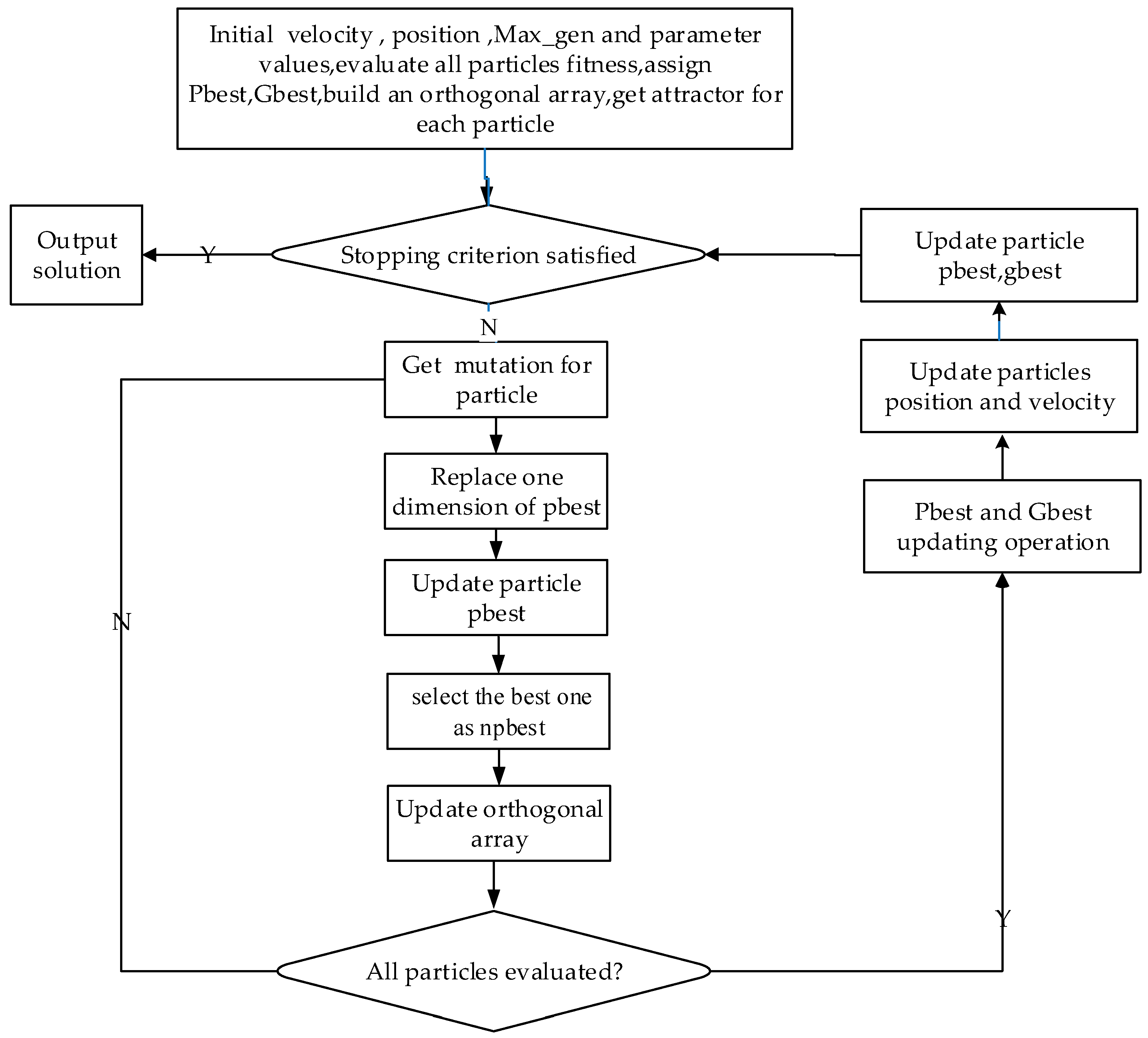
The detailed procedure of QPSO is shown in Algorithm 1. The framework of the proposed QPSO lies in the strategy to construct local attractors for particles. In QPSO, a particle uses the collaborative learning strategy to acquire a local attractor only if its local best position pbest_i has been held. The procedure of QPSO is shown in Algorithm 1. The flowchart of QPSO is shown in Figure 2.

Algorithm 1. Procedure of QPSO

1: Initialize (a) P(t) = (p1, p2, …, pn); % Pt is particle population, each particle in Pt is randomly initialized within the range of the searching space (b) Fit(Pt) = FitnessCalculation(Pt); % Calculate the fitness values of Pt (c) pbest(t) = P(t); % The personal best population is initialized as Pt (d) gbest(t) = FindBest(Pbest(t)); % gbest is the best individual in pbesti (e) For each particle pi, let stayi = 0; % stayi represents the number of generations for which particle pi has stays 2: Get attractori for each individual pi (a) If stayi ≤ G, then get attractori according to Equation (22); (b) stayi > G then %collaborative learning strategy ①: For pbesti, get k mutation individuals by Equation (23). ②: For each dimension j of pbesti, do (i) Replace the jth dimension of pbestj with that of the k individuals obtained in Step 1, respectively. Then, k new individuals (npbest1, npbest2, …, npbest(k)) are obtained. (ii) Get the fitness values of (npbest1, npbest2, …, npbest(t)) and select the best one as npbest. (iii) Take the jth dimension of best(t), pbest(t, as that of the attractori. 3: Update (a) Update P(t+1) according to (20) and (21); (b) Fit(t + 1) = Fitness Calculation(Pt + 1); % Calculate the fitness values of Pt+1; (c) If Fit(P(t)) is better than Fit(Pbest(t)), then Pbest(t+1) = P(t + 1) and stayi = 0. Otherwise, pbest(t + 1) = pbest(t)and stayi = stayi + 1; (d) gbest(t + 1) = FindBest(pbest(t + 1); % gbest(t + 1) is the best individual in Pbest(t + 1) 4: If the stop condition is satisfied, then output gbest. Otherwise, go to Step 2.

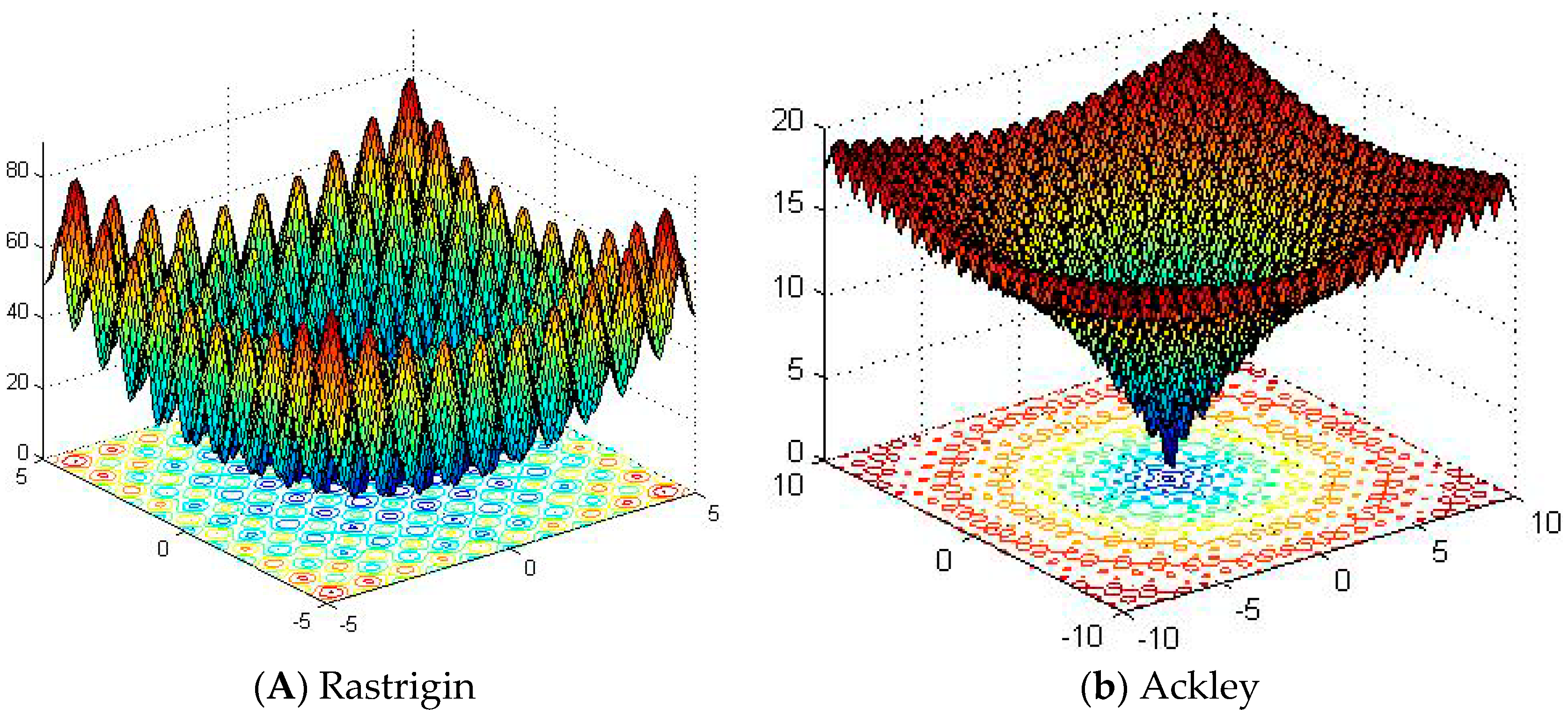
QE [19] and PSO [20,21,22,23] are two state-of-the-art algorithms. We choose two benchmarking functions to compare the results obtained by QE, PSO and QPSO; the results are representative and helpful to make the comparisons more comprehensive and convincing.

$$\begin{array}{l}R\mathrm{a}striginf(x)={\displaystyle {\sum }_{i=1}^n[x_i^2-10\cos (2\pi x_i)+10]}\\ f(x_i^{*})=0_{}x\in [-5.12,5.12]\\ Ackleyf(x)=-20\exp (-0.2\sqrt{\frac{1}{n}{\displaystyle {\sum }_{i=1}^n{x}_i^2}})-\exp (\frac{1}{n}{\displaystyle {\sum }_{i=1}^n\cos (2\pi x_i)})+20+\exp (1)\\ f(x_i^{*})=0_{}x\in [-32,32]\end{array}$$

The spatial characteristics of the test function are shown in Figure 3.

As can be seen from the test data in

Table 1. Function optimization test results. PSO: particle swarm optimization, QEA: quantum-inspired evolutionary algorithm.

Function		Best	Mean	Worst	STD	Gen(Mean)	Success
Restrigin	QEA	0	7.56 × 10−2	9.93 × 10−10	2.45 × 10−1	932	6
	PSO	0	1.08 × 10−11	2.01 × 10−10	4.02 × 10−11	845	27
	QPSO	0	0	0	0	46	32
Ackley	QEA	0	4.69 × 10−6	7.63 × 10−6	2.52 × 10−6	878	6
	PSO	0	0	0	0	742	37
	QPSO	0	0	0	0	34	30

, the optimal solution was found in all 30 independent runs of QPSO. The power is 100%. Compared with QEA and PSO, it has the ability to search for more accurate optimal value and find the optimal value. The number of iterations is much smaller than QEA and PSO.

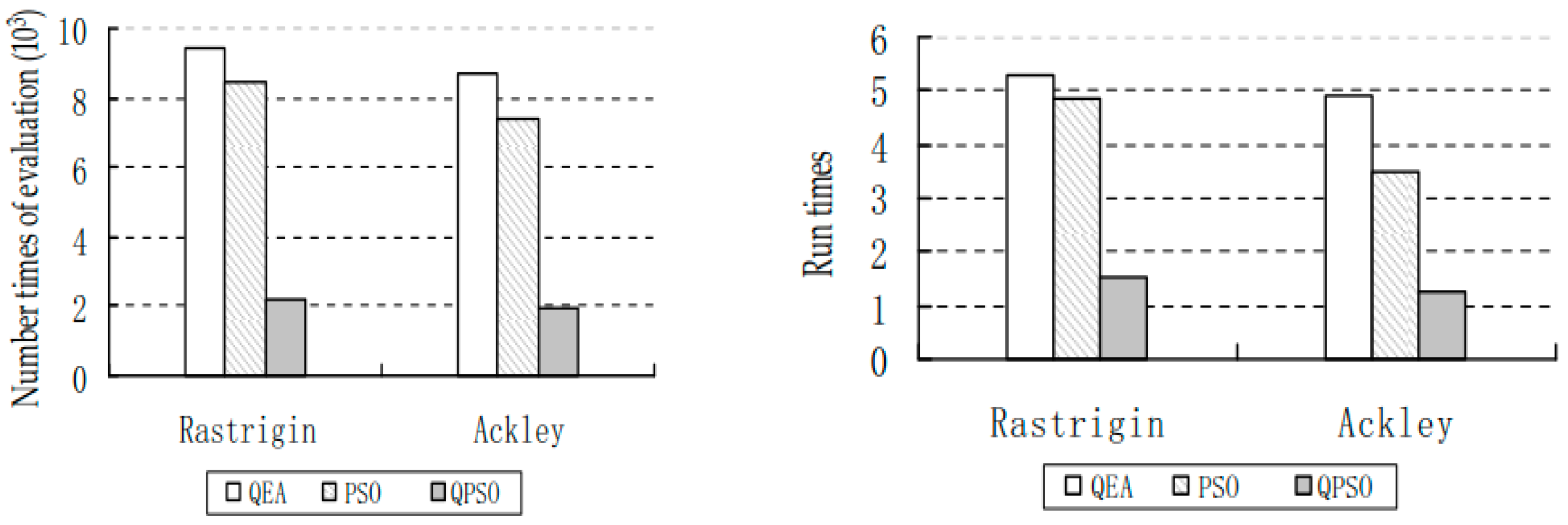
Figure 4 shows the average evaluation times and running time of three algorithms from 30 runs to the optimal solution. It can be seen that the number of times that QPSO finds the optimal solution is about 200 times, which is about four times less than QEA and PSO. However, the total running time decreased a lot. It can be seen that the time complexity of QPSO is significantly lower than that of QEA and PSO. Since the collaborative learning strategy prevents QPSO from falling into the local optimum trap, this adopted operator can control and achieve the balance between exploitation and exploration.

4. Case Study

The case study targets a large cold chain logistics enterprise in China. The enterprise runs many breading and processing facilities in southeastern China; it manages 13 large cold warehouses, with a total storage of 85,000 tons, and owns over 140 freezer cars. The distribution network of the enterprise covers most of the provinces and regions in China. As a comprehensive food processor, this enterprise engages in pig breeding, slaughtering, and processing, cold meat processing, and the manufacturing of meat products (e.g., canned food). The enterprise has set up a logistics subsidiary to integrate pig breeding, slaughtering, and processing, cold meat processing, and the manufacturing of meat products, aiming to improve the service levels, shorten the delivery times, and ensure product quality. Both economic and environmental factors were considered in the creation of a secondary supply chain network between the plants, distribution centers, and retailers.

Table 2. The maximum production capacity within the S cycle of the processing plant.

Manufacturer	Fuzhou	Zhuzhou	Chizhou
Maximum capacity (ton)	450	380	360

and

Table 3. Basic parameters of R.

R	Quantity Demanded (Unit: ton)	Service Level (%)	Demand Variance (Unit: ton)
Nanping	105	95%	14
Zhangzhou	118	95%	17
Taizhou	67	95%	11
Suzhou	87	95%	15
Hangzhou	98	95%	12
Taizhou	82	95%	14
Nanchang	120	95%	15
Pingxiang	86	95%	15
Fuyang	73	95%	13
Yichang	95	95%	12

present the maximum capacity per cycle (15 days) of the three food processing plants of the enterprises, assuming that the demand of each local retailer obeys normal distribution.

Table 4. Data of the distribution centers (DCs).

Potential Distribution Center (DC)	Maximum Storage Capacity (Unit: ton)	Construction Cost (Unit: yuan)	Unit Product Storage Cost (Unit: yuan/ton)
Zhuzhou	585	78,000	270
Sanming	590	79,000	240
Quzhou	520	76,000	270
Hefei	450	75,000	300
Nanjing	550	82,000	250
Fuzhou	640	811,000	210

presents the data of the distribution centers.

Table 5. The distance from the factory to the potential distribution center.

Factory	Zhuzhou	Sanming	Quzhou	Hefei	Nanjing	Fuzhou
Fuzhou	488	68	314	622	606	50
Zhuzhou	68	224	343	440	518	230
Chizhou	314	480	322	185	258	460

records the distribution of the demand per cycle of the 10 retailers.

Table 6. Factory to potential DC unit distance transportation costs.

	Zhuzhou	Sanming	Quzhou	Hefei	Nanjing	Fuzhou
Fuzhou	3.8	3.1	3.2	3.2	3.3	2.9
Zhuzhou	3.2	3.1	3.1	3.3	3.2	3.1
Chizhou	3.3	3.2	3.2	3.1	3.1	3.2

lists the data related to the regional distribution centers. For simplicity, the construction cost of each distribution center was calculated by the 24 cycles of each year. Table 3 and Table 4 respectively display the plant-distribution center distance, and the transport cost per unit of product. During the transport, the carbon emissions varied significantly with the congestion degree, road flatness, land slope, and fuel consumption. Therefore, the carbon emissions correlation coefficient which Hao employed for further analysis [24].

Table 7. Distance between potential distribution center and distributor.

	Retailer	Zhuzhou	Sanming	Quzhou	Hefei	Nanjing	Fuzhou
Distributor
Nanping		358	167	371	664	668	129
Zhangzhou		403	205	549	813	833	247
Taizhou		709	851	507	281	173	773
Suzhou		459	658	321	259	114	593
Hangzhou		451	497	149	325	244	446
Taizhou		411	361	158	537	486	291
Nanchang		91	318	373	376	485	325
Pingxiang		151	279	505	573	665	321
Fuyang		566	751	479	123	163	705
Yicheng		429	581	281	121	93	521

show the distribution center–retailer distance, and the transport distance per unit of product.

Table 8. DC to retailer (R) unit product unit distance transportation fee.

	Retailer	Zhuzhou	Sanming	Quzhou	Hefei	Nanjing	Fuzhou
Distributor
Nanping		3.8	3.1	3.2	3.4	3.3	3.1
Zhangzhou		3.3	3.2	3.3	3.3	3.4	3.2
Taizhou		3.5	3.2	3.2	3.2	3.3	3.2
Suzhou		3.2	3.2	3.3	3.2	3.2	3.2
Hangzhou		3.4	3.2	3.2	3.2	3.2	3.3
Taizhou		3.5	3.2	3.1	3.3	3.2	3.3
Nanchang		3.1	3.3	3.3	3.2	3.1	3.1
Pingxiang		3.1	3.1	3.4	3.4	3.3	3.2
Nanping		3.3	3.2	3.3	3.2	3.3	3.2
Zhangzhou		3.3	3.3	3.3	3.1	3.2	3.2

,

Table 9. The product unit of the factory to DC in carbon emissions.

	Retailer	Zhuzhou	Sanming	Quzhou	Hefei	Nanjing	Fuzhou
Factory
Fuzhou		0.11	0.08	0.09	0.09	0.08	0.09
Zhuzhou		0.05	0.11	0.08	0.08	0.05	0.11
Chizhou		0.08	0.09	0.05	0.08	0.05	0.11

and

Table 10. Carbon emissions of the DC to R unit product unit distance.

	Retailer	Zhuzhou	Sanming	Quzhou	Hefei	Nanjing	Fuzhou
Distributor
Nanping		0.12	0.12	0.1	0.12	0.08	0.12
Zhangzhou		0.12	0.12	0.1	0.12	0.08	0.12
Taizhou		0.08	0.08	0.06	0.08	0.06	0.08
Suzhou		0.08	0.1	0.08	0.12	0.06	0.08
Hangzhou		0.06	0.08	0.06	0.08	0.06	0.08
Taizhou		0.06	0.08	0.06	0.08	0.08	0.08
Nanchang		0.06	0.12	0.08	0.06	0.08	0.12
Pingxiang		0.06	0.12	0.08	0.08	0.12	0.12
Fuyang		0.08	0.08	0.08	0.12	0.06	0.08
Yicheng		0.08	0.08	0.08	0.08	0.06	0.07

respectively present the relationship between carbon emissions and the energy consumption per unit of product and the unit of distance for the plant–distribution center and distribution center–retailer.

Table 11. DC fixed carbon emissions and variable unit storage carbon emissions.

Potential Distribution Center	Fixed Carbon Emission (Unit: kg)	Unit Storage Carbon Emission (Unit: kg/ton)
Zhuzhou	790	0.46
Sanming	780	0.43
Quzhou	750	0.48
Hefei	740	0.51
Nanjing	790	0.49
Fuzh	810	0.39

gives the fixed carbon emissions of the distribution centers and the variable carbon emissions of the plants and retailers.

In this case, each retailer can be supplied by multiple distribution centers, and each center can be supplied by multiple plants. Then, the proposed model was applied to simulate this case on Matlab 7.1. The simulation parameters are as follows: the carbon emissions limit = 10,000 kg, the carbon penalty coefficient = 10, the service level = 95%, the inventory safety coefficient = 1.65, and the pre-order period = 6d. The simulated results (e.g., the optimal total cost, the economic cost, the carbon emissions, and the carbon emissions penalty) are presented in

Table 12. Distribution center to distributor.

Open DC	Distribution Center Responsible for Distributor Production	Supply (Unit: ton)	Base–DC–R Path
Fuzhou	Nanping distributor	161	Fuzhou–Nanping–Zhangzhou–Fuzhou–Taizhou
	Zhangzhou distributor	114
	Taizhou distributor	107
Nanjing	Taizhou distributor	95	Chizhou–Nanjing–Taizhou–Suzhou–Hangzhou–Wuhu
	Suzhou distributor	149
	Hangzhou distributor	165
	Fuyang distributor	96
	yicheng Distributor	49
Zhuzhou	Nanchang distributor	102	Zhuzhou–Pingxiang–Nanchang
	Pingxiang distributor	85

and

Table 13. Cost and carbon emissions calculations.

Total Cost (yuan)	Economic Cost (yuan)	Carbon Emission (kg)	Exceeds Carbon Emissions	Carbon Penalty Cost (yuan)	Carbon Cost Ratio
1,417,264.5	1,407,330.2	29,885.4	19,885.4	19,885.4	12.3%

below.

The calculation shows in Table 12 reveals that the distribution of the whole supply chain relies on the regional distribution centers of Fuzhou, Nanjing and Huzhou. As shown in Table 13, the total cost, the economic cost, the carbon emissions, and the excess carbon emissions were respectively 1,417,264.5 yuan, 1,407,330.2 yuan, 29,885.4 kg, and 19,885.4 kg. Hence, the carbon emissions penalty accounts for 12.3% of the total cost.

Table 14. Transportation of the plant to the selected distribution center.

The Factory	The Factory Supplies the Selected Distribution Center	Supply (Unit: ton)
Fuzhou	Fuzhou distribution center	392
Chizhou	Nanjing distribution center	554
Zhuzhou	Zhuzhou distribution center	187

shows the quantity of products delivered from each distribution center to each retailer. It can be seen that the Fuzhou distribution center delivers products to Nanping, Zhangzhou, and Taizhou, with the inventory safety coefficient of 195.7 tons; the Nanjing distribution center delivers products to Taizhou, Suzhou, Hangzhou, Fuyang, and Yichang, with the inventory safety coefficient of 243.9 tons, the Zhuzhou distribution center delivers products to Nanchang and Pingxiang, with the inventory safety coefficient of 195.7 tons.

According to the

Table 15. The location scheme and total cost change under different carbon penalty coefficients.

Carbon Penalty Coefficient	10	20	30	40
Optimal site selection scheme.	Fuzhou, Nanjing, Zhuzhou	Nanjing, Fuzhou	Nanjing, Fuzhou	Zhuzhou, Quzhou
Total supply chain cost (yuan)	1,656,184.2	1,757,690.5	1,921,039.5	2,095,279.4
Economic cost (yuan)	1,457,330.2	1,470,336.5	1,470,337.5	1,501,223.4
Carbon emission (kg)	29,885.4	24,367.7	25,023.4	26,451.4
Exceeding the carbon emission limit.	19,885.4	14,367.7	15,023.4	14,851.4
Carbon emission cost (yuan)	198,854	287,354	450,702	594,056
Proportion of carbon cost (%)	12.0	16.3	23.5	28.4

, when the carbon emissions limit was 10,000 kg and the carbon emissions penalty coefficient was 10, the optimal distribution plan involves three distribution centers: Fuzhou, Nanjing, and Zhuzhou. When the carbon emissions limit was 10,000 kg and the carbon emissions penalty coefficient was 20, the optimal distribution plan involves two distribution centers: Nanjing and Fuzhou. Comparing the two optimal plans, the two-center plan reduced the total cost by 101,506.3 yuan, increased the economic cost by 13,006.3 yuan and lowered carbon emissions by 5517.7 kg from the level of the three-center plan. In addition, when the carbon emissions limit was 10,000 kg and the carbon emissions penalty coefficient was 30, the optimal distribution plan involves two distribution centers: Nanjing and Nanping. When the carbon emissions limit was 10,000 kg and the carbon emissions penalty coefficient was 40, the optimal distribution plan involves two distribution centers, they are Fuzhou and Hefei. Comparing the two optimal plans, the second plan increased the total cost by 174,239.9 yuan, reduced the economic cost by 30,885.9 yuan, and reduced the carbon emissions by 172 kg from the level of the first plan. Summing up, the whole supply chain will emit less CO₂ by increasing the carbon emissions penalty.

Furthermore, according to the

Table 16. Site selection scheme and total cost change under different carbon limits.

Carbon Quotas (kg)	30,000	25,000	20,000
Optimal site selection scheme.	Fuzhou, Nanjing, Zhuzhou	Nanjing, Fuzhou	Nanjing, Fuzhou
Total supply chain cost (yuan)	1,457,330.2	1,470,336.5	1,511,472.5
Economic cost (yuan)	1,457,330.2	1,470,336.5	1,470,337.5
Carbon emission (kg)	29,885.4	24,367.7	24,113.5
Exceeding the carbon emission limit.	0	0	4113.5
Carbon emission cost (yuan)	0	0	41,135

, when the carbon emissions limit was 30,000 kg and the carbon emissions penalty coefficient was 10, the optimal distribution plan involves three distribution centers: Fuzhou, Nanjing, and Zhuzhou. In this case, the carbon emissions (29,885.4 kg) was below the carbon emissions limit, indicating that the carbon emissions penalty was zero. When the carbon emissions limit was adjusted to 25,000 kg, the optimal plan involved two distribution centers: Nanjing and Fuzhou. In this case, the carbon emissions (24,367.7 kg) was still below the carbon emissions limit, and thus the carbon emissions penalty remained zero. Meanwhile, the carbon emissions dropped to 5517.7 kg. When the carbon emissions limit was lowered to 20,000 kg, the optimal plan still involved two distribution centers: Nanjing and Fuzhou. However, the carbon emissions (241,135.5 kg) exceeded the limit, leading to a penalty of 41,135 yuan. Therefore, the reduction of carbon emissions limit can pressurize the enterprise to cut down the carbon emissions of the supply chain through low-carbon design.

Overall, the total cost of the supply chain increased with the reduction of the carbon emissions limit and the growth in the carbon emissions penalty coefficient. These laws will help enterprises optimize the design of supply chain network, making it possible to strike a balance between economic benefit and environmental effect.

5. Conclusions

It is common in the logistics and supply chain that the objectives of decreasing logistic costs, carbon emissions, and increasing energy efficiency are targeted at the multi-level of the supply chain’s members. This work has developed a methodology based on heuristic optimization to minimize the logistics costs and carbon emissions based on relevant constraints, which aims to improve enterprise’s interests.

The described model represents an integrated optimization problem including the assignment of open tasks to scheduled routes, the scheduling of open tasks, and there scheduling of existing delivery routes. The optimization problem, which is described by an objective function representing the minimization of the logistic costs and carbon emissions and constraints, including loading capacity limits and time frames, is a hard problem. For the solution of this problem, a quantum-particle swarm optimization-based heuristic was developed. The developed heuristic is an improved version of the quantum-inspired evolutionary algorithm and basic particle swarm optimization; its increased performance is validated with benchmarking functions.

The integrated optimization model of the real-time scheduling of a multi-echelon logistics problem is solved with these heuristics. As the scenarios showed, cooperation makes it possible to increase the energy efficiency through the minimization of carbon emissions under different constraints. In the case of package delivery service providers, the time frame and the loading capacity of the package delivery trucks are important constraints; as the mentioned scenarios show, they are influencing their reliability, availability, flexibility, and economic footprints.

The described model framework and the optimization approach make it possible to support managerial decisions; not only the operation strategy of the running trucks, but also the cooperation strategy of different package delivery service providers are influenced by the results of the above described contribution. Some recommendations for possible future studies are as follows: it would be helpful to develop approaches that are beyond analyzing scheduling and assignment possibilities and also consider other areas of interest, such as human resource strategies, delivery truck sizing, out sourcing possibilities, or the rate of carbon tax.

References

- Yang, C.S.; Lu, C.S.; Xu, J.; Marlow, P.B. Evaluating green supply chain management capability, environmental performance, and competitiveness in container shipping context. J. East. Asia Soc. Transp. Stud. 2013, 10, 2274–2293. [Google Scholar]
- Bányai, T.; Illés, B.; Bányai, Á. Smart scheduling: An integrated first mile and last mile supply approach. Complexity 2018. [Google Scholar] [CrossRef]
- Bányai, T.; Sciubba, E. Real-Time Decision Making in First Mile and Last Mile Logistics: How Smart Scheduling Affects Energy Efficiency of Hyperconnected Supply Chain Solutions. Energies 2018, 11, 1833. [Google Scholar] [CrossRef]
- Kadadevaramath, R.S.; Chen, J.C.H.; LathaShankar, B.; Rameshkumar, K. Application of particle swarm intelligence algorithms in supply chain network architecture optimization. Expert Syst. Appl. 2012, 39, 10160–10176. [Google Scholar] [CrossRef]
- Tamás, P. Innovative business model for realization of sustainable supply chain at the outsourcing examination of logistics services. Sustainability 2018, 10, 210. [Google Scholar] [CrossRef]
- Figliozzi, M.A. Lifecycle modeling and assessment of unmanned aerial vehicles (Drones) CO2 emissions. Transp. Res. Part D Transp. Environ. 2017, 57, 251–261. [Google Scholar] [CrossRef]
- Bazan, E.; Jaber, M.Y.; Zanoni, S. Carbon emissions and energy effects on a two-level manufacturer-retailer closed-loop supply chain model with remanufacturing subject to different coordination mechanisms. Int. J. Prod. Econ. 2016, 183, 394–408. [Google Scholar] [CrossRef]
- Tobias, S.; Sachin, B.M.; Benton, W.C.; Craig, R.C.; Thomas, Y.C.; Paul, D.L. Research opportunities in purchasing and supply management. Int. J. Prod. Res. 2012, 50, 4556–4579. [Google Scholar] [Green Version]
- Liou, J.J.H.; Tamošaitienė, J.; Zavadskas, E.K.; Tzeng, G.-h. New hybrid COPRAS-G MADM Model for improving and selecting suppliers in green supply chain management. Int. J. Prod. Res. 2016, 54, 114–134. [Google Scholar] [CrossRef]
- Al-E-Hashem, S.M.J.M.; Baboli, A.; Sazvar, Z. A stochastic aggregate production planning model in a green supply chain: Considering flexible lead times, nonlinear purchase and shortage cost functions. Eur. J. Oper. Res. 2013, 230, 26–41. [Google Scholar] [CrossRef]
- Fleischmann, B.; Meyr, H.; Wagner, M. Supply Chain Management and Advanced Planning, 4th ed.; Springer: Berlin, Germany, 2010; pp. 81–106. [Google Scholar]
- Amorim, P.; Almada-Lobo, B.; Barbosa-Póvoa, A.P.F.D.; Grossmann, I.E. Combining supplier selection and production-distribution planning in food supply chains. Comput. Aided Chem. Eng. 2014, 33, 409–414. [Google Scholar]
- Goha, M.; Limb, J.Y.S.; Mengc, F. A stochastic model for risk management in global supply chain networks. Eur. J. Oper. Res. 2007, 182, 164–173. [Google Scholar] [CrossRef]
- Sarkis, J. Policy insights from a green supply chain optimization model. Int. J. Prod. Res. 2015, 53, 6522–6533. [Google Scholar]
- Hedayati, M.; Firouzeh, Z.H.; Nekoei, H.K. Hybrid quantum particle swarm optimization to calculate wideband green’s functions for microstrip structures. IET Microw. Antennas Propag. 2016, 10, 264–270. [Google Scholar] [CrossRef]
- Wu, D.; Zheng, J. A dynamic multistage hybrid swarm intelligence optimization algorithm for function optimization. Discret. Dyn. Nat. Soc. 2012, 2012, 1951–1965. [Google Scholar] [CrossRef]
- Wu, D.Q.; Dong, M.; Li, H.Y. Vehicle routing problem with time windows using multi-objective co-evolutionary approach. Int. J. Simul. Model. 2016, 15, 742–753. [Google Scholar] [CrossRef]
- Sun, J.; Fang, W.; Wu, X.; Palade, V.; Xu, W. Quantum-behaved particle swarm optimization: Analysis of individual particle behavior and parameter selection. Evol. Comput. 2012, 20, 349–393. [Google Scholar] [CrossRef] [PubMed]
- Gao, H.; Zhang, R. Real-coded Quantum Evolutionary Algorithm for Global Numerical Optimization with Continuous Variables. Chin. J. Electron. 2011, 20, 499–503. [Google Scholar]
- Khan, S.U.; Yang, S.; Wang, L.; Liu, L. A modified particle swarm optimization algorithm for global optimizations of inverse problems. IEEE Trans. Magn. 2016, 52, 1–4. [Google Scholar] [CrossRef]
- Deng, W.; Zhao, H.; Zou, L.; Li, G.; Yang, X.; Wu, D. A novel collaborative optimization algorithm in solving complex optimization problems. Soft Comput. 2017, 21, 4387–4398. [Google Scholar] [CrossRef]
- Huang, J.; Shuai, Y.; Liu, Q.; Zhou, H.; He, Z. Synergy Degree Evaluation Based on Synergetics for Sustainable Logistics Enterprises. Sustainability 2018, 10. [Google Scholar] [CrossRef]
- Wang, D.F.; Dong, Q.L.; Peng, Z.M.; Khan, S.A.R.; Tarasov, A. The Green Logistics Impact on International Trade: Evidence from Developed and Developing Countries. Sustainability 2018, 10. [Google Scholar] [CrossRef]
- Guo, H.; Li, C.; Zhang, Y.; Zhang, C.; Lu, M. A Location-Inventory Problem in a Closed-Loop Supply Chain with Secondary Market Consideration. Sustainability 2018, 10, 1891. [Google Scholar] [CrossRef]
Figure 1.
The three-echelon supply chain network.
Figure 2.
The flowchart of QPSO.
Figure 3.
Two benchmarking functions.
Figure 4.
The result of two benchmarking functions.