Robust Day-Ahead Scheduling of Electricity and Natural Gas Systems via a Risk-Averse Adjustable Uncertainty Set Approach


1
School of Electrical Engineering, Xi’an Jiaotong University, Xi’an 710049, China
2
State Grid Zhejiang Electric Power Co., LTD., Hang Zhou 310007, China
*
Author to whom correspondence should be addressed.
Sustainability 2018, 10(11), 3848; https://doi.org/10.3390/su10113848
Submission received: 8 October 2018
/
Revised: 19 October 2018
/
Accepted: 20 October 2018
/
Published: 24 October 2018
(This article belongs to the Collection Power System and Sustainability)
Abstract
:The requirement for energy sustainability drives the development of renewable energy technologies and gas-fired power generation. The increasing installation of gas-fired units significantly intensifies the interdependency between the electricity system and natural gas system. The joint scheduling of electricity and natural gas systems has become an attractive option for improving energy efficiency. This paper proposes a robust day-ahead scheduling model for electricity and natural gas system, which minimizes the total cost including fuel cost, spinning reserve cost and cost of operational risk while ensuring the feasibility for all scenarios within the uncertainty set. Different from the conventional robust optimization with predefined uncertainty set, a new approach with risk-averse adjustable uncertainty set is proposed in this paper to mitigate the conservatism. Furthermore, the Wasserstein–Moment metric is applied to construct ambiguity sets for computing operational risk. The proposed scheduling model is solved by the column-and-constraint generation method. The effectiveness of the proposed approach is tested on a 6-bus test system and a 118-bus system.
1. Introduction
The climate change and global warming concerns coupled with high oil prices and government support are driving increasing integration of variable renewable energies into the power system [1]. Renewable energies have many advantages including reducing environmental pollution, bringing economic benefits, improving energy efficiency, and enhancing life quality [2].
The ongoing shale gas revolution is expected to slash nature gas prices and attract investment into gas-fired power generation. Take California’s generation mix as an example, natural gas provided approximately 53 percent of total installed capacity which is the largest source of energy to meet the load [3]. The increasing installation of gas-fired units significantly intensifies the interdependency between the electricity system and natural gas system. On one hand, gas-fired units can offer flexible dispatch and quick ramping capability [4]. On the other hand, the gas outages or gas shortage damage the reliability of power system as gas-fired units go off-line [5].
The joint scheduling of electricity and natural gas infrastructures has become an attractive option for improving the energy efficiency of the whole system [6]. In recent years, there have been many works dedicated to the joint optimal scheduling of the integrated energy system. Some studies are summarized as follows:
(1) Gas Flow Modeling: In order to ensure the computational tractability, the Weymouth equation is widely adopted to describe the relationship between gas flow and gas pressure under the steady-state assumption. Liu et al. propose a security-based methodology for the solution of short-term SCUC with considering the impact of the natural gas transmission system by using natural gas transmission subproblem to check the feasibility as well as the security [7]. In reference [8], authors develop a novel gas flow model such that line pack, i.e., the stored gas in the pipeline, is taken into account. That paper contributes with an extended incremental method that linearizes the nonlinear term in the Weymouth equation. However, such method introduces a large number of additional variables/constraints, posing a high computational burden to the solver. In paper [9], the Weymouth equation is convexified via a second order cone relaxation method, but the exactness of the relaxation cannot be guaranteed. In references [10,11], natural gas transmission is simplified by linear constraints, making the complex gas transmission problem tractable.
(2) Uncertainty Modeling: The increasing integration of variable renewable energy (VRE) into the power system brings uncertainties to the operation, which may result in load shedding, grid instability and potentially, cascading outages. In the scope of this paper, the VREs’ power output is the only source of uncertainties. How to manage the VREs’ uncertainties is a hot issue in the research field of joint scheduling. Alabdulwahab et al. build a scenario-based stochastic scheduling model for the electricity and natural gas systems [12]. A decomposition method is designed to check the feasibility of gas transmission problem in all the scenarios. In reference [13], the operation of a GB integrated gas and electricity network considering the wind power uncertainty is investigated using three operational methods: deterministic, two-stage stochastic programming, and multistage stochastic programming. Based on the interval optimization, Bai et al. propose a joint scheduling model with considering an optimal demand response strategy [14]. With resorting to the robust optimization method, He et al. propose a robust co-optimization scheduling model to study the coordinated optimal operation of the integrated energy systems [15]. That paper is tackled via an alternating direction method of multipliers (ADMM) by iteratively solving a power system subproblem. In this way, the privacy of data is protected.
In the existing literature focusing on joint scheduling, stochastic programming and robust optimization are two popular tools for addressing uncertainties. Stochastic programming assumes that the distribution governing the uncertainty data is known or can be estimated in advance. In contrast, robust optimization assumes that the probabilistic information is not available, and only the upper and lower bounds of uncertainty variables are determined [16]. Therefore, robust optimization may lead to an over-conservative decision. Recently, a novel optimization tool, named ’distributionally robust optimization’, is proposed to bridge the gap between stochastic programming and robust optimization. It constructs an ambiguity set containing the possible distributions of random variables. Then, it optimizes the expected cost under the worst-case distribution within the ambiguity set. In references [17,18], authors establish the moment-based ambiguity set where the moment information of possible distributions is consistent with that of the empirical distribution. A statistical distance-based metric– Wasserstein metric is employed in paper [19,20,21] to construct the ambiguity set.
This paper proposes a robust day-ahead scheduling model for electricity and natural gas system, which minimizes the total cost including fuel cost, spinning reserve cost and cost of operational risk while ensuring the feasibility for all scenarios within the uncertainty set. The proposed model is a two-stage robust optimization model. The base-case plan (base-case power output of units and preserved spinning reserve capacity) and the parameters of adjustable uncertainty set are determined in the first stage, while carrying out redispatch in the second stage after the realizations of uncertainties are revealed. Follow the study in [10], a simplification model is utilized to model the gas transmission with considering the line pack. The proposed model adopts an adjustable uncertainty set approach proposed in [22]. However, to hedge against the ambiguity of distribution, this paper proposes a risk-averse adjustable uncertainty set approach that computes the operational risk under the worst-case distribution by a distributionally robust method. Different from our previous work [23], this paper builds the ambiguity set via a Wasserstein–Moment metric [24,25]. Comparative studies are carried out to compute operational risk among the Wasserstein–Moment metric, Wasserstein metric, and Moment metric. In addition, this paper aims to coordinate different energy infrastructures but not the power system modeled in [23]. Our study has the following major contributions:
(1) We co-optimize energy and reserve for day-ahead scheduling in electricity and natural gas system. The gas transmission problem is simplified for achieving computational tractability.
(2) A risk-averse adjustable uncertainty set approach is proposed to mitigate the conservatism of robust optimization. To overcome distribution ambiguity, we construct the ambiguity set using a Wasserstein–Moment metric. Then, operational risk is the expected value under the worst-case distribution within such ambiguity set.
2. Methodology
The flowchart of the proposed method is shown in Figure 1. First, we collect the historical data of forecasting errors. Then, based on the Wasserstein–Moment Metric, DRO models are constructed to compute the operational risk. By tuning the bounds of adjustable uncertainty set, we can form the operational risk curve for each VRE plant. Secondly, we build the robust day-ahead scheduling model for electricity and natural gas systems using the risk-averse adjustable uncertainty set approach. Such a model can be solved via the column-and-constraint generation method.
2.1. Risk-Averse Adjustable Uncertainty Set Approach
As the forecasting system has been an effective tool to predict the power output of VRE plant j, the forecasting error is the random variable which is denoted as . Suppose that we have a historical dataset for with sample size N, i.e., . Let and represent the sample mean and the sample standard deviation of , respectively. We can construct an adjustable uncertainty set :
where is a variable used to tune the scope of . According to the definition of robust optimization, for all the scenarios within the , the redispatch feasibility should be ensured. In other words, any scenario falling outside the may cause the operational loss ([22,23]). In statistical decision theory, the risk function is defined as the expected value of a given loss function as a function of the decisions in the face of uncertainty. Following such definition, when fixing the decision as , the operational risk is defined as an expected value of the operational loss under the empirical distribution , shown as follow:
where and are the wind power curtailment price and load shedding price, respectively. Nonetheless, it may result in a suboptimal solution, in particular in the case when limited historical data are available. To solve this problem, we construct an ambiguity set to contain the possible distribution with calculating the operational risk under the worst-case distribution in such ambiguity set. The corresponding operational risk is:
This paper introduces a Wasserstein–Moment metric ([24,25]) to construct an ambiguity set where represents the empirical distribution formed by .
where is the function to compute the Wasserstein distance between two distributions; denotes the set containing all the possible distributions of ; is a parameter to control conservatism, which can be obtained by the cross-validation method [17]. In this paper, the parameter is chosen as follow [20]:
where S represents the diameter of the support of random variable; the parameter is set as 0.9, implying that the ambiguity set is able to cover the true distribution with the probability of . According to Theorem 1, the operational risk w.r.t. can be obtained by solving a semi-definite linear program.
Theorem 1.
Suppose that random variable has a convex support where and are column vectors. The worst expectation of operational risk (3) is equivalent to:
The proof can be derived from a lemma provided in the appendix of our prior work [25]. If we parameterize the adjustable variable as a linear interpolation of a sequence of fixed values, , ,...,. Accordingly, by using Theorem 1, we obtain a sequence of possible operational risk, , ,.... Despite the fact that is a nonlinear function of , it can be approximated by the piecewise linear function shown as follows:
where and are auxiliary continuous variable and binary variable w.r.t. the mth interval of piecewise linear curve. Constraint (15) ensures that there will be at most one index m where we have . Any given point can be uniquely represented by (12), as a linear combination of two consecutive breakpoints weighted by the associated variables . The nonlinear function is then approximated by the model as convex combination of the function values evaluated at the breakpoints weighted by the associated variables . Hereinafter, for simplicity, model (12)–(15) is written to the general formulation:
Through (16), we can plot an operational risk curve which describes the as the function of . Obviously, increasing enlarges the scope of the adjustable uncertainty set, resulting in a lower operational risk. That is, is a non-increasing function of .
2.2. Robust Day-Ahead Scheduling Model for Electricity and Natural Gas System
The proposed model aims to minimize the total cost including fuel cost, spinning reserve cost and cost of operational risk while satisfying the operating constraints. Since the operational risk is explicitly added in the objective function, the decision-maker achieves the optimal decision by making a tradeoff between economics and reliability. Denote to represent the set of gas-fired units. Let be the set of non-gas thermal units. represents the set of VRE plant. denotes the set of gas wells. The objective function is written as below:
where is the fuel cost of unit i at time t; is the gas price for gas well k; and are the downward spinning reserve and upward spinning reserve, respectively; and are the spinning reserve price; is the operational risk w.r.t. VRE plant j at time t, which is calculated as discussed in Section 2.
2.2.1. First-Stage Constraints
In the first stage, the decision-maker optimizes the decision related to the base-case dispatch plan. The constraints are given as follows:
(1) Fuel cost of non-gas thermal unit i at time t.
The fuel cost curve is approximated by the piecewise linear function.
where and are the slope and intercept of the s-th segment; is the base-case power output of unit i; is the binary variable representing the state of unit i.
(2) Power balance constraints.
where is the forecasted power output of VRE plant j; is the forecasted power of load at bus b; is the set of buses.
(3) Power output limits:
where and are the lower limit and upper limit of power output of unit i, respectively.
(4) Spinning reserve limits:
where and are the lower limit and the upper limit of spinning reserve of unit i, respectively.
(5) Transmission line capacity contraints
where , , and are the power transfer distribution factors from unit i, VRE plant j, and load at bus b to line l, respectively. and are capacity limits of line l.
(6) Gas consumption of gas-fired units.
For gas-fired unit i, its gas consumption depends on power output . In order to develop the piecewise linear approximation of such functional relationship, let us divide the axis over the range of function to -1 segments using m = 1,2,... breakpoints , ,... . Each mth interval is associated with a continuous variable and a binary variable .
where and denote the slope and intercept of the m-th segment. Constraint (26) ensures that only one binary variable can take the value 1, and thus only one segment is active. Constraint (24) and (25) enforce that is equal to if mth segment is active, otherwise .
(7) Gas nodal balance constraint.
where is the gas load at node ; represents the set of pipelines connected with gas node ; denotes the set of gas-fired units plugged at node ; is the set of gas well at node ; is the gas flow injecting into node from pipeline . We note that is positive when gas flow runs from pipeline to , otherwise it is a negative value.
(8) Line pack temporal constraints.
Line pack refers to the quantity of natural gas stored in the pipeline. Line pack can be used to smooth the real-time gas demand variation and maintain gas pressure stability.
where denotes the origin node of pipeline ; denotes the destination node of pipeline ; is the linepack of pipeline at time t.
(9) Line pack/gas supply/outgoing gas flow limits constraints.
where the upper bound and lower bound of a variable is written with an overline and an underline.
(10) Initial line pack constraints.
Constraints (32) enforce the initial line pack is equal to the final line pack to facilitate the daily operation.
(11) Constraints associated with operational risk, i.e., constraints (16).
2.2.2. Second-Stage Constraints
After VREs’ power outputs are realized, system operators carry out corrective actions e.g., redispatching and load shedding. According to the definition of robust optimization, any scenario within the adjustable uncertainty set will not violate the operating constraints.
(1) Real-time released spinning reserve.
The real-time adjustment of generators should be within its spinning reserve preserved in the first stage.
where and are the upward corrective power and downward corrective power, respectively.
(2) Real-time power balance.
where () represents the adjustable uncertainty set w.r.t. VRE plant j at time t.
(3) Real-time transmission line capacity.
(4) Real-time gas consumption of gas-fired unit i
For gas-fired unit i, the real-time gas consumption is assumed to be a linear function of the real-time power output at the active segment ().
where M is a sufficient large constant; is the real-time gas consumption. We mention that decision are obtained in the first stage. It can be seen from constraint (36) that for the active segment (), we have
while constraint (36) is relaxed for other inactive segments.
In the second stage, there are constraints associated with the real-time operating of the gas system, which is similar to the constraints shown in (27)–(32). For simplicity, we do not present them here.
The proposed joint scheduling model is written into the compact form:
where is the vector of variables in the first stage; is the vector of variables in the second stage; is the feasible region formed by the constraints in the first stage; is the vector of the operational risks ; is the vector of random variables; is the vector of the parameters ; and are vectors of sample means and sample standard deviations ; is the union of uncertainty sets ; ’∘’ denotes the Hadamard product. Matrices , and , and represent the parameters in the second-stage constraints. Constraints (40) correspond to the second-stage constraints.
2.3. Solution Methodology
The proposed joint scheduling model can be solved by column and constraints generation algorithm (C&CG) which has been proved to be an efficient solution methodology for two-stage robust optimization model [26]. Next, we briefly discuss the solution methodology. Interested readers can refer to our previous work [23] for detailed information.
Given the fixed first-stage decision , the C&CG subproblem aims to identify the worse-case scenario by solving the following model:
where is a vector of relaxation variables. With introducing the uncertainty budget and to mitigate the conservatism of robust optimization, the above model is reformulated to the following model by dual theory:
where binary column vectors and are indicators of the bounds of ; is the vector of dual variables; is the spatial budget; is the temporal budget. When the subproblem is solved in the kth iteration, denoting the optimal solution of and as and , respectively, a set of extra variables , and additional constraints are generated as shown in (21) and added to the master problem.
Suppose that K iterations have been proceeded, the C&CG master problem is given as follows:
The above iterative process will continue until the optimal value of subproblem is 0, which means that all the scenarios within the adjustable uncertainty set are feasible.
3. Numerical Results
Numerical tests on the integrated energy system including a 6-bus power system and a 6-node natural gas system is carried out as an illustrative example. A larger system containing an IEEE 118-bus power system and a 10-node natural gas system are used to verify the computational efficiency of the proposed method. The semi-definite linear programs are solved with MOSEK, and mixed integer linear programming models are solved with GUROBI. All the tests are performed on a PC, which has 8GB memory and i7-4790 CPU.
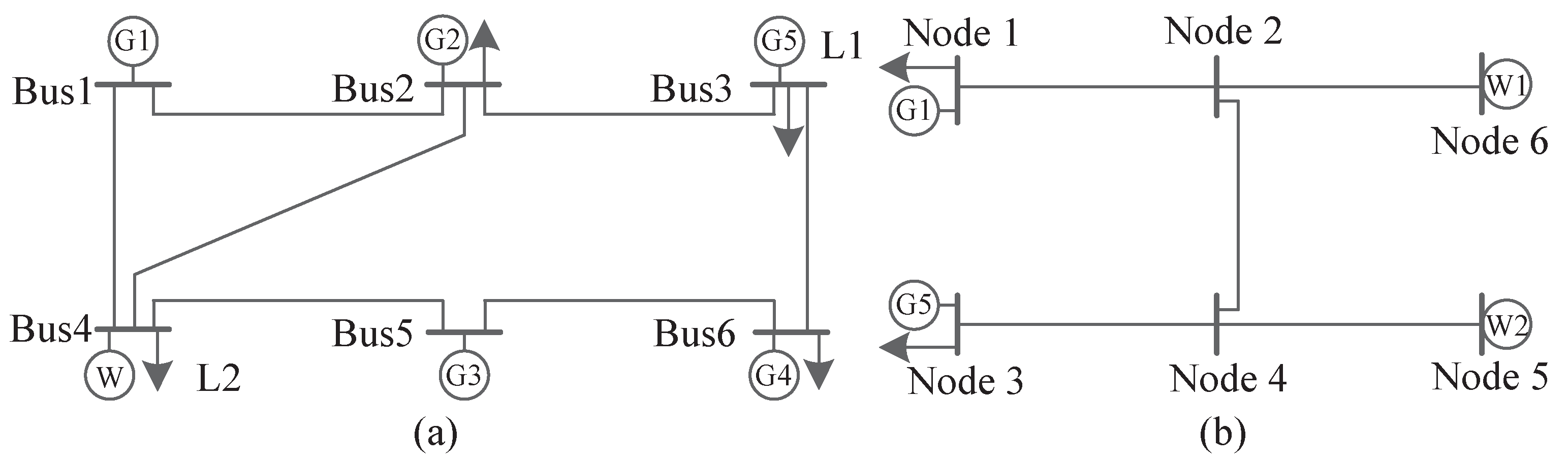
3.1. Six-Bus Power System with a 6-Node Natural Gas System
We use the test system in [15] with a trivial modification. The topologies are shown in Figure 2. The 6-bus power system includes non-gas thermal units G2–G4, gas-fired units G1 and G5, a wind farm connecting to bus 4, seven transmission lines, and three loads. Fuel price of G2–G4 is 5 $/MBtu. The 6-node gas system comprises two gas wells, five pipelines, and four gas loads. The wind power curtailment prices and load shedding prices are assumed to vary with time periods, which are plotted in Figure 3. The total power loads and total gas loads are also illustrated in Figure 3. Data for this integrated energy system are provided in [27]. Budget and are set as 1 and 24, respectively.
A wind farm is connected to the power system at bus 4 with a capacity of 240 MW. The forecasted power output is plotted in Figure 4. Following the setting in [22], the forecasting error of wind generation is assumed to follow a Gaussian distribution where the mean value is 0 and the standard deviation is:
where is the forecasted power output of VRE plant j. We make the assumption on the ’true’ distribution to sample data for constructing ambiguity sets. In this way, instead of the ’true’ distribution, the sampled data are available for the decision-making and thus the proposed approach essentially does not rely on the specified distributions.
The simulation procedure is given as follows: (1) Sample N = 5000 data from the assumed ’true’ Gaussian distribution for constructing ambiguity sets; (2) The typical points on the operational risk curve are determined by solving (6)–(11); (3) Build the optimization model and solve it; (4) By keeping the base-case plan fixed, calculate the expected total cost under the ’true’ distribution to test the out-of-sample performance of the decision.
In order to investigate the conservatism of Wasserstein–Moment-metric (WM-metric), we introduce moment-metric (M-metric) [17] and Wasserstein-metric (W-metric) [23]. All tests are based on the same sample set for fair comparison. Monte Carlo Simulation (MCS) with samples is employed to provide the benchmark for comparison. Then, based on several metrics, the operational risk curves at hour 1 and hour 24 are plotted in the Figure 5.
From Figure 5, it can be seen that WM-metric is the most aggressive one among the studied metrics. The reason is that both of statistical distance and moment information are taken into account, reducing the ambiguity of random variables. In general, the more probabilistic information is used to construct the ambiguity set, the worst-case distribution will be less conservative.
Based on the above operational risk curves, the following four cases are used to investigate the performance of WM-metric in making dispatch decision:
Case 1: Conventional two-stage robust optimization model where the parameters of predefined uncertainty sets are selected as in [28] (95% confidence intervals are adopted);
Case 2: Proposed scheduling model with WM-metric;
Case 3: Proposed scheduling model with W-metric;
Case 4: Proposed scheduling model with M-metric;
The unit commitment decision is illustrated in Figure 6. It is observed that Cases 2–4 result in the same decision while Case 1 commits more unit in hour 1, 2, 3 and 23. It indicates that the conventional two-stage robust model with unadjustable uncertainty set leads to a more conservative decision compared with the proposed model. Cases 2–4 yield different spinning reserve solutions. Figure 7 shows the total upward spinning reserve for each hour. Case 2 preserves significantly less spinning reserve than other cases due to its less conservative estimation of operational risk. The downward spinning reserve in these cases is not shown here because we come to similar conclusions.
The results of costs are shown in Table 1. We compare two types of total costs. The first type is the estimated total cost which is the sum of the production cost (fuel cost and spinning reserve cost) and operational risk cost. Actually, the first type cost is the objective value of (17). By fixing the base-case dispatch plan, we solve the re-dispatch problem with samples generated from the assumed distribution, and record the expected risk cost including load shedding cost and wind power curtailment cost. The second type total cost, named simulated total cost, is equal to the sum of the production cost and expected risk cost.
From Table 1, it can be seen that Case 2 achieves the lowest production cost as well as the total cost. The reason is that the spinning reserve scheduled in Case 2 is less than that in other cases as shown in Figure 7. Compared with other cases, the production cost is reduced in Case 2 at the price of increasing the risk cost. However, Case 2 compromises reliability due to the lowest total cost. It is suggested that using WM-metric is able to mitigate the conservatism of the risk-averse adjustable uncertainty set approach so that Case 2 makes the best tradeoff between economics and reliability among all the cases.
Next, we investigate the effect of gas shortage on the unit commitment. We assume that some contingencies restrict the capacity of the pipeline directed from node 1 to node 2 so that gas supply cannot satisfy the demand of the gas-fired unit at node 1. As a result, this gas-fired unit cannot be committed but replaced by costly non-gas thermal units. Under such assumption, the unit commitment decision is presented in Figure 8 . Cases 2–4 lead to the same feasible decision while Case 1 is not feasible, implying that the adjustable uncertainty set approach can be a promising alternative method in particular cases when the conventional robust methods cannot provide a feasible solution.
Table 2 summarizes the costs for each case. Case 2 also achieves the lowest total cost as in Table 1. From the comparison between Table 1 and Table 2, we can find that the total costs are greatly increased because of the shutdown of cost-efficient unit 1. It indicates that the gas shortage severely reduces the operation efficiency of the integrated enery system.
3.2. IEEE 118-Bus Power System with a 10-Node Natural Gas System
We use this system to test the computational performance of the proposed method. The modified IEEE-118 bus power system consists of 46 non-gas thermal units, eight gas-fired units, six wind farms, 186 branches, and 91 loads. We simplify the gas system in [15] by reducing storage facilities and compressors. The modified gas system includes ten gas nodes, three gas wells, ten pipelines, and 12 gas loads. Six wind farms are connected to the system at buses 12, 17, 49, 59, 80, and 92 with a capacity of 200 MW for each bus. Uncertainty budget is set as 3 to reduce conservatism, which means that there are at most three wind farms simultaneously experience fluctuations. The four cases studied in the previous subsection are carried out, the results are listed in Table 3. Like the results in the 6-bus test system, the scheduling model with WM-metric is less conservative than other models and achieves a better balance between reliability and economics.
We obtain the operational risk curves in the preparation stage. These problems are highly parallelizable among different time periods and wind farms, and therefore, we can speed up the computation via solving these problems in a parallel manner. Owing to the parallel manner, time costs are listed in Table 4. For all the cases, the time costs spent on solving scheduling models are comparable. Nonetheless, Case 2 spends more time forming operational risk curves than other cases because it is inefficient to tackle semi-definite programming constraints.
4. Conclusions
This paper proposes a robust day-ahead scheduling model for electricity and natural gas systems, which minimizes the total cost including fuel cost, spinning reserve cost and cost of operational risk while ensuring the feasibility for all scenarios within the uncertainty set. From the numerical results, we conclude that:
- (1)
- The proposed scheduling model can coordinate different energy infrastructures to improve the energy efficiency of the electricity and natural gas system. The gas shortage has a significant adverse impact on the economic efficiency.
- (2)
- The risk-averse adjustable uncertainty set approach can be a promising alternative method in particular cases when the conventional robust methods cannot provide a feasible solution.
- (3)
- Compared with the other two metrics, WM-metric helps to reduce the conservatism of risk-averse adjustable uncertainty set approach.
- (4)
- The proposed scheduling model can be solved efficiently via the C&CG algorithm.
The proposed method can be used by the system operator to execute day-ahead joint scheduling (or market clearing) of the electricity and natural gas systems. The performance of the proposed method highly depends on the data quality because available data are used to construct ambiguity sets for computing operational risk. In this regard, the data cleaning and the outliers detection method can be utilized to improve data quality. The proposed method does not specify the type of VRE plant, but deals with the random forecasting error. Therefore, it also can be applied to the system that includes other renewable units such as solar PV and biomass units, etc.
Author Contributions
Methodology, L.Y.; Writing—original draft, L.Y.; Project administration, X.W.; Supervision, X.W.; Software, T.Q.; Writing – review & editing, S.Q. and C.Z.
Funding
This research was funded by State Grid Science & Technology Project: Research on Morphologies and Pathways of Future Power Systems.
Conflicts of Interest
The authors declare no conflict of interest.
References
- Kung, C.C.; McCarl, B.A. Sustainable Energy Development under Climate Change. Sustainability 2018, 10, 3269. [Google Scholar] [CrossRef]
- Ntanos, S.; Kyriakopoulos, G.; Chalikias, M.; Arabatzis, G.; Skordoulis, M.; Galatsidas, S.; Drosos, D. A Social Assessment of the Usage of Renewable Energy Sources and Its Contribution to Life Quality: The Case of an Attica Urban Area in Greece. Sustainability 2018, 10, 1414. [Google Scholar] [CrossRef]
- Daneshi, H. Overview of Renewable Energy Portfolio in CAISO—Operational and Market Challenges. In Proceedings of the 2018 IEEE PES General Meeting (PESGM), Portland, OR, USA, 5–9 August 2018. [Google Scholar]
- Zhang, X.; Che, L.; Shahidehpour, M.; Alabdulwahab, A.; Abusorrah, A. Electricity-Natural Gas Operation Planning With Hourly Demand Response for Deployment of Flexible Ramp. IEEE Trans. Sustain. Energy 2016, 7, 996–1004. [Google Scholar] [CrossRef]
- Fedora, P.A. Reliability review of North American gas/electric system interdependency. In Proceedings of the 37th Annual Hawaii International Conference on System Sciences, Big Island, HI, USA, 5–8 January 2004; pp. 1–10. [Google Scholar]
- Ye, J.; Yuan, R. Integrated Natural Gas, Heat, and Power Dispatch Considering Wind Power and Power-to-Gas. Sustainability 2018, 9, 602. [Google Scholar] [CrossRef]
- Liu, C.; Shahidehpour, M.; Fu, Y.; Li, Z. Security-constrained unit commitment with natural gas transmission constraints. IEEE Trans. Power Syst. 2009, 24, 1523–1536. [Google Scholar]
- Correa-Posada, C.M.; Sánchez-Martín, P. Integrated Power and Natural Gas Model for Energy Adequacy in Short-Term Operation. IEEE Trans. Power Syst. 2017, 30, 3347–3355. [Google Scholar] [CrossRef]
- Correa-Posada, C.M.; Sánchez-Martín, P. Robust Constrained Operation of Integrated Electricity-Natural Gas System Considering Distributed Natural Gas Storage. IEEE Trans. Sustain. Energy 2018, 9, 1061–1071. [Google Scholar]
- Liu, C.; Lee, C.; Shahidehpour, M. Look Ahead Robust Scheduling of Wind-Thermal System With Considering Natural Gas Congestion. IEEE Trans. Power Syst. 2015, 30, 544–545. [Google Scholar] [CrossRef]
- Zhao, B.; Conejo, A.J.; Sioshansi, R. Unit Commitment Under Gas-Supply Uncertainty and Gas-Price Variability. IEEE Trans. Power Syst. 2017, 32, 2394–2405. [Google Scholar] [CrossRef]
- Alabdulwahab, A.; Abusorrah, A.; Zhang, X.; Shahidehpour, M. Coordination of Interdependent Natural Gas and Electricity Infrastructures for Firming the Variability of Wind Energy in Stochastic Day-Ahead Scheduling. IEEE Trans. Sustain. Energy 2015, 6, 606–615. [Google Scholar] [CrossRef]
- Alabdulwahab, A.; Abusorrah, A.; Zhang, X.; Shahidehpour, M. Operating Strategies for a GB Integrated Gas and Electricity Network Considering the Uncertainty in Wind Power Forecasts. IEEE Trans. Sustain. Energy 2013, 5, 128–138. [Google Scholar]
- Bai, L.; Li, F.; Cui, H.; Jiang, T.; Sun, H.; Zhu, J. Interval optimization based operating strategy for gas-electricity integrated energy systems considering demand response and wind uncertainty. Appl. Energy 2016, 167, 270–279. [Google Scholar] [CrossRef] [Green Version]
- He, C.; Wu, L.; Liu, T.; Shahidehpour, M. Robust co-optimization scheduling of electricity and natural gas systems via ADMM. IEEE Trans. Sustain. Energy 2017, 8, 658–670. [Google Scholar] [CrossRef]
- Bertsimas, D.; Litvinov, E.; Sun, X.A.; Zhao, J.; Zheng, T. Adaptive Robust Optimization for the Security Constrained Unit Commitment Problem. IEEE Trans. Power Syst. 2013, 28, 52–63. [Google Scholar] [CrossRef] [Green Version]
- Delage, E.; Ye, Y. Distributionally Robust Optimization Under Moment Uncertainty with Application to Data-Driven Problems. Oper. Res. 2010, 58, 595–612. [Google Scholar] [CrossRef] [Green Version]
- Wei, W.; Liu, F.; Mei, S. Distributionally Robust Co-Optimization of Energy and Reserve Dispatch. IEEE Trans. Sustain. Energy 2016, 7, 289–300. [Google Scholar] [CrossRef]
- Mohajerin Esfahani, P.; Kuhn, D. Data-driven distributionally robust optimization using the Wasserstein metric: Performance guarantees and tractable reformulations. Math. Program. 2018, 171, 1–52. [Google Scholar] [CrossRef]
- Zhao, C.; Guan, Y. Data-driven risk-averse stochastic optimization with Wasserstein metric. Oper. Res. Lett. 2018, 46, 262–267. [Google Scholar] [CrossRef]
- Duan, C.; Fang, W.; Jiang, L.; Yao, L.; Liu, J. Distributionally robust chance-constrained approximate ac-opf with wasserstein metric. IEEE Trans. Power Syst. 2018, 33, 4924–4936. [Google Scholar] [CrossRef]
- Wang, C.; Liu, F.; Wang, J.; Wei, W.; Mei, S. Risk-Based Admissibility Assessment of Wind Generation Integrated into a Bulk Power System. IEEE Trans. Sustain. Energy 2016, 7, 325–336. [Google Scholar] [CrossRef]
- Yao, L.; Wang, X.; Duan, C.; Guo, J.; Wu, X.; Zhang, Y. Data-driven distributionally robust reserve and energy scheduling over Wasserstein balls. IET Gener. Transm. Distrib. 2018, 12, 178–189. [Google Scholar] [CrossRef]
- Gao, R.; Kleywegt, A.J. Distributionally robust stochastic optimization with dependence structure. arXiv, 2017; arXiv:1701.04200. [Google Scholar]
- Yao, L.; Wang, X.; Duan, C.; Wu, X.; Zhang, W. Risk-based Distributionally Robust Energy and Reserve Dispatch with Wasserstein–Moment Metric. In Proceedings of the 2018 IEEE PES General Meeting (PESGM), Portland, OR, USA, 5–9 August 2018. [Google Scholar]
- Zeng, B.; Zhao, L. Solving two-stage robust optimization problems using a column-and-constraint generation method. Oper. Res. Lett. 2013, 41, 457–461. [Google Scholar] [CrossRef]
- 6-Bus Power System with a 6-Node Natural Gas System. Available online: https://docs.google.com/spreadsheets/d/1PL9pnwLO1hdkDmZFkTLIVNCA4P_5vgOqxXh24Y\xJEHk/edit?usp=sharing (accessed on 28 September 2018).
- Guan, Y.; Wang, J. Uncertainty Sets for Robust Unit Commitment. IEEE Trans. Power Syst. 2014, 291, 1439–1440. [Google Scholar] [CrossRef]
Figure 1.
Flowchart of the proposed method.

Figure 2.
(a) 6-bus power system; (b) 6-node natural gas system.

Figure 3.
(a) Load shedding prices/wind power curtailment prices; (b) Power loads/Gas loads.

Figure 4.
Forecasted wind power output.

Figure 5.
Operational risk curves: (a) t = 1; (b) t = 24.

Figure 6.
Unit commitment decision for Cases 1–4.

Figure 7.
Upward spinning reserve for Cases 1–4.

Figure 8.
Unit commitment decision for gas shortage example.


Table 1.
Results of costs (k$).
| Case | Production Cost | Estimated Total Cost | Simulated Total Cost | ||
|---|---|---|---|---|---|
| Operational Risk Cost | Total Cost | Expected Loss Cost | Total Cost | ||
| Case 1 | 589.7 | \ | 589.7 | 0.2 | 589.9 |
| Case 2 | 581.0 | 6.6 | 587.6 | 2.5 | 583.5 |
| Case 3 | 589.3 | 1.5 | 590.8 | 0.3 | 589.6 |
| Case 4 | 588.4 | 2.3 | 590.7 | 0.5 | 588.9 |
Table 2.
Results of costs for gas shortage example (k$).
| Case | Production Cost | Estimated Total Cost | Simulated Total Cost | ||
|---|---|---|---|---|---|
| Operational Risk Cost | Total Cost | Expected Loss Cost | Total Cost | ||
| Case 1 (infeasible) | \ | \ | \ | \ | \ |
| Case 2 | 891.0 | 13.1 | 904.1 | 8.1 | 899.1 |
| Case 3 | 889.9 | 20.4 | 910.3 | 9.2 | 899.1 |
| Case 4 | 892.9 | 17.9 | 910.8 | 6.7 | 899.6 |
Table 3.
Results of costs in a larger system (k$).
| Case | Production Cost | Estimated Total Cost | Simulated Total Cost | ||
|---|---|---|---|---|---|
| Operational Risk Cost | Total Cost | Expected Loss Cost | Total Cost | ||
| Case 1 | 10,262.4 | \ | 10,262.4 | 1.1 | 10,263.5 |
| Case 2 | 10,248.1 | 13.1 | 10,261.2 | 5.2 | 10,253.3 |
| Case 3 | 10,254.5 | 9.9 | 10,264.4 | 3.1 | 10,257.6 |
| Case 4 | 10,257.2 | 7.4 | 10,264.6 | 2.8 | 10,260.0 |
Table 4.
Computational efficiency.
| Case | Time of Preparation (s) | Time of C & CG (s) |
|---|---|---|
| Case 1 | \ | 91.2 |
| Case 2 | 921 | 125.1 |
| Case 3 | 54 | 114.4 |
| Case 4 | 10.9 | 102.9 |
© 2018 by the authors. Licensee MDPI, Basel, Switzerland. This article is an open access article distributed under the terms and conditions of the Creative Commons Attribution (CC BY) license (http://creativecommons.org/licenses/by/4.0/).
Share and Cite
MDPI and ACS Style
Yao, L.; Wang, X.; Qian, T.; Qi, S.; Zhu, C. Robust Day-Ahead Scheduling of Electricity and Natural Gas Systems via a Risk-Averse Adjustable Uncertainty Set Approach. Sustainability 2018, 10, 3848. https://doi.org/10.3390/su10113848
AMA Style
Yao L, Wang X, Qian T, Qi S, Zhu C. Robust Day-Ahead Scheduling of Electricity and Natural Gas Systems via a Risk-Averse Adjustable Uncertainty Set Approach. Sustainability. 2018; 10(11):3848. https://doi.org/10.3390/su10113848
Chicago/Turabian StyleYao, Li, Xiuli Wang, Tao Qian, Shixiong Qi, and Chengzhi Zhu. 2018. "Robust Day-Ahead Scheduling of Electricity and Natural Gas Systems via a Risk-Averse Adjustable Uncertainty Set Approach" Sustainability 10, no. 11: 3848. https://doi.org/10.3390/su10113848
Note that from the first issue of 2016, this journal uses article numbers instead of page numbers. See further details here.