The Effect of Observation Scale on Urban Growth Simulation Using Particle Swarm Optimization-Based CA Models

Abstract
:1. Introduction
2. Study Area and Data
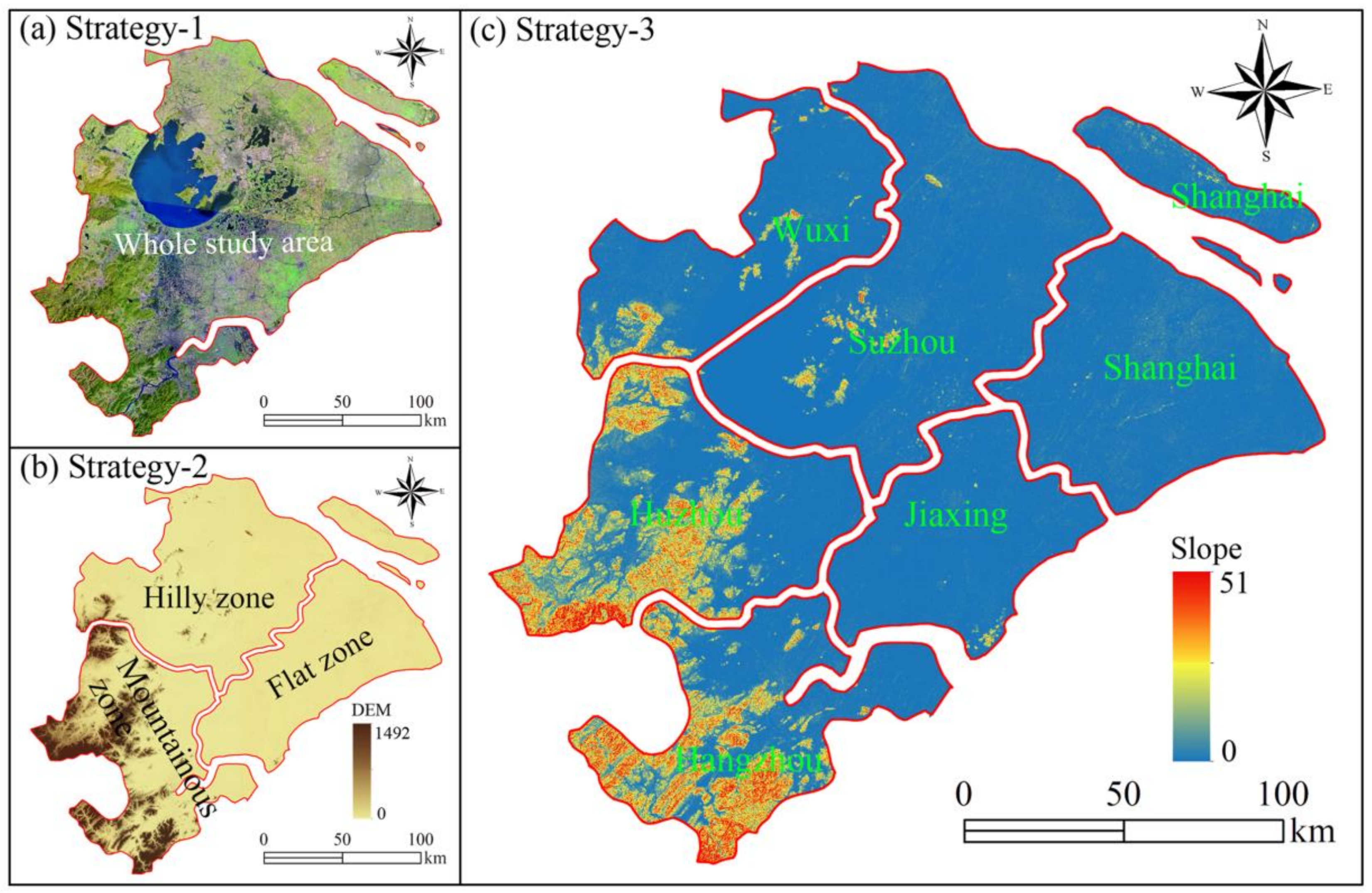
2.1. The Study Area: UA-Shanghai
2.2. Raw Data and Spatial Variables
3. PSO-CA Modeling
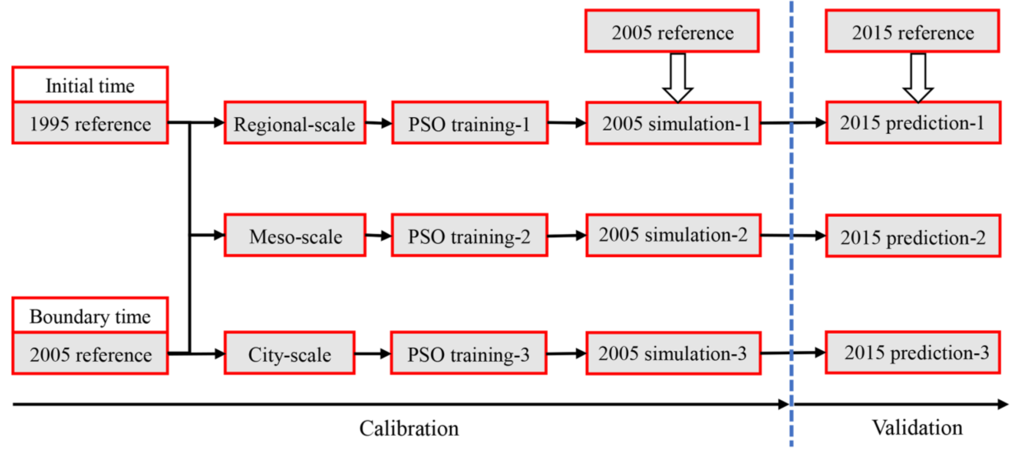
3.1. Workflow
3.2. The PSO-CA Model
3.3. Validation Methods
4. Results
4.1. Transition Rules and Land Transition Probability Maps
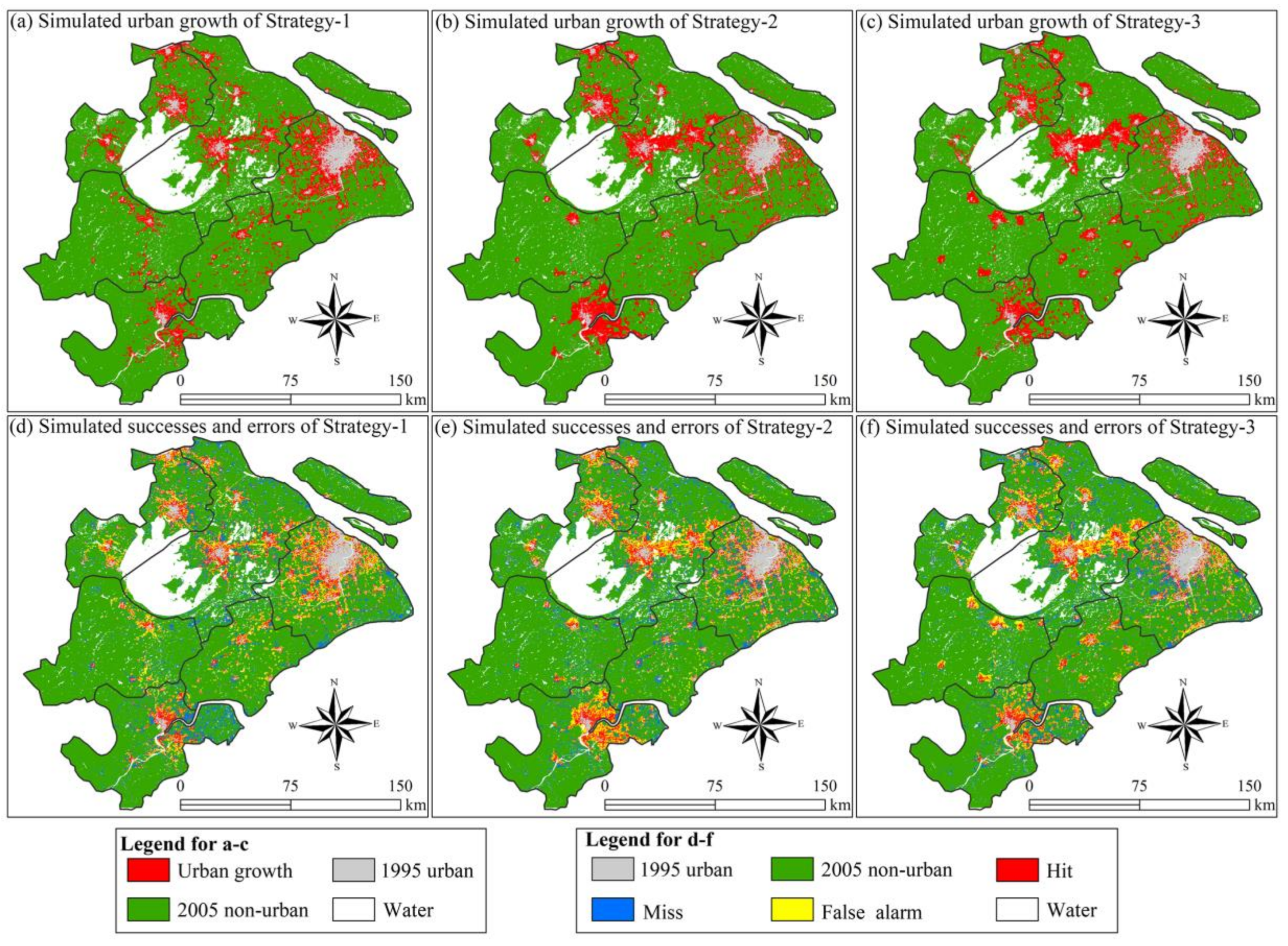
4.2. The Simulation and Prediction Results
4.3. Relationship between Simulation Accuracy and Urban Growth Rate
4.4. Discussion
5. Conclusions
Author Contributions
Funding
Acknowledgments
Conflicts of Interest
References
- Ebrahimipour, A.; Saadat, M.; Farshchin, A. Prediction of urban growth through cellular automata-markov chain. Bull. Soc. R. Sci. Liège 2016, 85, 824–839. [Google Scholar]
- Sakieh, Y.; Amiri, B.J.; Danekar, A.; Feghhi, J.; Dezhkam, S. Simulating urban expansion and scenario prediction using a cellular automata urban growth model, sleuth, through a case study of Karaj city, Iran. J. Hous. Built Environ. 2015, 30, 591–611. [Google Scholar] [CrossRef]
- Bozkaya, A.G.; Balcik, F.B.; Goksel, C.; Esbah, H. Forecasting land-cover growth using remotely sensed data: A case study of the Igneada protection area in Turkey. Environ. Monit. Assess. 2015, 187, 59. [Google Scholar] [CrossRef] [PubMed]
- Hamad, R.; Balzter, H.; Kolo, K. Predicting land use/land cover changes using a ca-markov model under two different scenarios. Sustainability 2018, 10, 3421. [Google Scholar] [CrossRef]
- Wang, R.; Derdouri, A.; Murayama, Y. Spatiotemporal simulation of future land use/cover change scenarios in the Tokyo metropolitan area. Sustainability 2018, 10, 2056. [Google Scholar] [CrossRef]
- Liu, X.; Liang, X.; Li, X.; Xu, X.; Ou, J.; Chen, Y.; Li, S.; Wang, S.; Pei, F. A future land use simulation model (flus) for simulating multiple land use scenarios by coupling human and natural effects. Landsc. Urban Plan. 2017, 168, 94–116. [Google Scholar] [CrossRef]
- Osman, T.; Divigalpitiya, P.; Arima, T. Driving factors of urban sprawl in giza governorate of the greater cairo metropolitan region using a logistic regression model. Int. J. Urban Sci. 2016, 20, 206–225. [Google Scholar] [CrossRef]
- Kamusoko, C.; Aniya, M.; Adi, B.; Manjoro, M. Rural sustainability under threat in zimbabwe–simulation of future land use/cover changes in the bindura district based on the markov-cellular automata model. Appl. Geogr. 2009, 29, 435–447. [Google Scholar] [CrossRef]
- Chakraborti, S.; Das, D.N.; Mondal, B.; Shafizadeh-Moghadam, H.; Feng, Y. A neural network and landscape metrics to propose a flexible urban growth boundary: A case study. Ecol. Indic. 2018, 93, 952–965. [Google Scholar] [CrossRef]
- Pan, Y.; Roth, A.; Yu, Z.; Doluschitz, R. The impact of variation in scale on the behavior of a cellular automata used for land use change modeling. Comput. Environ. Urban Syst. 2010, 34, 400–408. [Google Scholar] [CrossRef]
- Ménard, A.; Marceau, D.J. Exploration of spatial scale sensitivity in geographic cellular automata. Environ. Plan. B Plan. Des. 2005, 32, 693–714. [Google Scholar] [CrossRef]
- Lau, K.H.; Kam, B.H. A cellular automata model for urban land-use simulation. Environ. Plan. B Plan. Des. 2005, 32, 247–263. [Google Scholar] [CrossRef]
- Cheng, J.; Masser, I. Understanding spatial and temporal processes of urban growth: Cellular automata modelling. Environ. Plan. B Plan. Des. 2004, 31, 167–194. [Google Scholar] [CrossRef]
- Jantz, C.A.; Goetz, S.J. Analysis of scale dependencies in an urban land-use-change model. Int. J. Geogr. Inf. Sci. 2005, 19, 217–241. [Google Scholar] [CrossRef]
- Lin, Y.P.; Chu, H.J.; Wu, C.F.; Verburg, P.H. Predictive ability of logistic regression, auto-logistic regression and neural network models in empirical land-use change modeling-a case study. Int. J. Geogr. Inf. Sci. 2011, 25, 65–87. [Google Scholar] [CrossRef] [Green Version]
- Feng, Y.; Liu, Y.; Tong, X.; Liu, M.; Deng, S. Modeling dynamic urban growth using cellular automata and particle swarm optimization rules. Landsc. Urban Plan. 2011, 102, 188–196. [Google Scholar] [CrossRef]
- Berling-Wolff, S.; Wu, J. Modeling urban landscape dynamics: A case study in phoenix, USA. Urban Ecosyst. 2004, 7, 215–240. [Google Scholar] [CrossRef]
- Kocabas, V.; Dragicevic, S. Assessing cellular automata model behaviour using a sensitivity analysis approach. Comput. Environ. Urban Syst. 2006, 30, 921–953. [Google Scholar] [CrossRef]
- Wu, H.; Chi, X.; Li, Y.; Sun, Y. Quantifying and analyzing neighborhood configuration characteristics to cellular automata for land use simulation considering data source error. Earth Sci. Inform. 2012, 5, 77–86. [Google Scholar] [CrossRef]
- Liao, J.; Tang, L.; Shao, G.; Su, X.; Chen, D.; Xu, T. Incorporation of extended neighborhood mechanisms and its impact on urban land-use cellular automata simulations. Environ. Model. Softw. 2016, 75, 163–175. [Google Scholar] [CrossRef]
- Liu, X.; Hu, G.; Chen, Y.; Li, X.; Xu, X.; Li, S.; Pei, F.; Wang, S. High-resolution multi-temporal mapping of global urban land using landsat images based on the google earth engine platform. Remote. Sens. Environ. 2018, 209, 227–239. [Google Scholar] [CrossRef]
- Alqurashi, A.F.; Kumar, L.; Al-Ghamdi, K.A. Spatiotemporal modeling of urban growth predictions based on driving force factors in five Saudi Arabian cities. ISPRS Int. J. Geo-Inf. 2016, 5, 139. [Google Scholar] [CrossRef]
- Al-shalabi, M.; Billa, L.; Pradhan, B.; Mansor, S.; Al-Sharif, A.A. Modelling urban growth evolution and land-use changes using gis based cellular automata and sleuth models: The case of sana’a metropolitan city, Yemen. Environ. Earth Sci. 2013, 70, 425–437. [Google Scholar] [CrossRef] [Green Version]
- Arsanjani, J.J.; Helbich, M.; Kainz, W.; Boloorani, A.D. Integration of logistic regression, markov chain and cellular automata models to simulate urban expansion. Int. J. Appl. Earth Obs. Geoinf. 2013, 21, 265–275. [Google Scholar] [CrossRef]
- Feng, Y.; Liu, Y.; Tong, X. Comparison of metaheuristic cellular automata models: A case study of dynamic land use simulation in the Yangtze river delta. Comput. Environ. Urban Syst. 2018, 70, 138–150. [Google Scholar] [CrossRef]
- Fan, F.; Wang, Y.; Wang, Z. Temporal and spatial change detecting (1998–2003) and predicting of land use and land cover in core corridor of Pearl river delta (China) by using tm and etm+ images. Environ. Monit. Assess. 2008, 137, 127. [Google Scholar] [CrossRef] [PubMed]
- Pijanowski, B.C.; Tayyebi, A.; Doucette, J.; Pekin, B.K.; Braun, D.; Plourde, J. A big data urban growth simulation at a national scale: Configuring the GIS and neural network based land transformation model to run in a high performance computing (HPC) environment. Environ. Model. Softw. 2014, 51, 250–268. [Google Scholar] [CrossRef]
- Agarwal, C.; Green, G.M.; Grove, J.M.; Evans, T.P.; Schweik, C.M. A review and assessment of land-use change models: Dynamics of space, time, and human choice. In General Technical Report; U.S. Department of Agriculture, Forest Service, Northeastern Research Station: Newton Square, PA, USA, 2002. [Google Scholar]
- Ke, X.; Qi, L.; Zeng, C. A Partitioned and Asynchronous Cellular Automata Model for Urban Growth Simulation; Taylor & Francis, Inc.: Milton Park, FL, USA, 2016; pp. 637–659. [Google Scholar]
- Rabbani, A.; Aghababaee, H.; Rajabi, M.A. Modeling dynamic urban growth using hybrid cellular automata and particle swarm optimization. J. Appl. Remote Sens. 2012, 6, 3582. [Google Scholar] [CrossRef]
- Yao, F.; Hao, C.; Zhang, J. Simulating urban growth processes by integrating cellular automata model and artificial optimization in Binhai new area of Tianjin, China. Geocarto Int. 2015, 31, 612–627. [Google Scholar] [CrossRef]
- National Development and Reform Commission of China. Urban Agglomeration Development Planning of the Yangtze River Delta; National Development and Reform Commission of China: Beijing, China, 2016. [Google Scholar]
- Li, X.; Zhou, W.; Ouyang, Z. Forty years of urban expansion in Beijing: What is the relative importance of physical, socioeconomic, and neighborhood factors? Appl. Geogr. 2013, 38, 1–10. [Google Scholar] [CrossRef] [Green Version]
- Hu, Y.; Zhang, Y.; Ke, X. Dynamics of tradeoffs between economic benefits and ecosystem services due to urban expansion. Sustainability 2018, 10, 2306. [Google Scholar] [CrossRef]
- Li, X.; Wang, M.; Liu, X.; Chen, Z.; Wei, X.; Che, W. Mcr-modified ca–markov model for the simulation of urban expansion. Sustainability 2018, 10, 3116. [Google Scholar] [CrossRef]
- Mitsova, D.; Shuster, W.; Wang, X. A cellular automata model of land cover change to integrate urban growth with open space conservation. Landsc. Urban Plan. 2011, 99, 141–153. [Google Scholar] [CrossRef]
- Rienow, A.; Goetzke, R. Supporting sleuth–enhancing a cellular automaton with support vector machines for urban growth modeling. Comput. Environ. Urban Syst. 2015, 49, 66–81. [Google Scholar] [CrossRef]
- Han, J.; Hayashi, Y.; Cao, X.; Imura, H. Application of an integrated system dynamics and cellular automata model for urban growth assessment: A case study of Shanghai, China. Landsc. Urban Plan. 2009, 91, 133–141. [Google Scholar] [CrossRef]
- He, C.; Li, J.; Zhang, X.; Liu, Z.; Zhang, D. Will rapid urban expansion in the drylands of northern china continue: A scenario analysis based on the land use scenario dynamics-urban model and the shared socioeconomic pathways. J. Clean. Prod. 2017, 165, 57–69. [Google Scholar] [CrossRef]
- Munshi, T.; Zuidgeest, M.; Brussel, M.; Maarseveen, M.V. Logistic regression and cellular automata-based modelling of retail, commercial and residential development in the city of Ahmedabad, India. Cities 2014, 39, 68–86. [Google Scholar] [CrossRef]
- Liu, Y.; Feng, Y.; Pontius, R.G. Spatially-explicit simulation of urban growth through self-adaptive genetic algorithm and cellular automata modelling. Land 2014, 3, 719–738. [Google Scholar] [CrossRef]
- Dessel, W.V.; Rompaey, A.V.; Szilassi, P. Sensitivity analysis of logistic regression parameterization for land use and land cover probability estimation. Int. J. Geogr. Inf. Sci. 2011, 25, 489–508. [Google Scholar] [CrossRef]
- Engelen, G.; White, R. Validating and calibrating integrated cellular automata based models of land use change. In the Dynamics of Complex Urban Systems; Springer: Berlin, Germany, 2008; pp. 185–211. [Google Scholar]
- Aguilera, F.; Valenzuela, L.M.; Botequilha-Leitão, A. Landscape metrics in the analysis of urban land use patterns: A case study in a Spanish metropolitan area. Landsc. Urban Plan. 2011, 99, 226–238. [Google Scholar] [CrossRef]
- Liu, Y.; Feng, Y. Simulating the impact of economic and environmental strategies on future urban growth scenarios in Ningbo, China. Sustainability 2016, 8, 1045. [Google Scholar] [CrossRef]
- Samat, N. Integrating GIS and ca-markov model in evaluating urban spatial growth. Malays. J. Environ. Manag. 2009, 10, 83–99. [Google Scholar]
- Aljoufie, M.; Zuidgeest, M.; Brussel, M.; Vliet, J.V.; Maarseveen, M.V. A cellular automata-based land use and transport interaction model applied to Jeddah, Saudi Arabia. Landsc. Urban Plan. 2013, 112, 89–99. [Google Scholar] [CrossRef]
- Wu, F. Calibration of stochastic cellular automata: The application to rural-urban land conversions. Int. J. Geogr. Inf. Sci. 2002, 16, 795–818. [Google Scholar] [CrossRef]
- García, A.M.; Santé, I.; Boullón, M.; Crecente, R. Calibration of an urban cellular automaton model by using statistical techniques and a genetic algorithm. Application to a small urban settlement of NW Spain. Int. J. Geogr. Inf. Sci. 2013, 27, 1593–1611. [Google Scholar] [CrossRef]
- Andries, P.E. Fundamentals of Computational Swarm Intelligence; Wiley: Hoboken, NJ, USA, 2006. [Google Scholar]
- Gao, L.; Huang, J.; Li, X. An effective cellular particle swarm optimization for parameters optimization of a multi-pass milling process. Appl. Soft Comput. J. 2012, 12, 3490–3499. [Google Scholar] [CrossRef]
- Clerc, M.; Kennedy, J. The particle swarm—Explosion, stability, and convergence in a multidimensional complex space. IEEE Trans. Evol. Comput. 2002, 6, 58–73. [Google Scholar] [CrossRef]
- Afshar, M.H. Extension of the constrained particle swarm optimization algorithm to optimal operation of multi-reservoirs system. Int. J. Electr. Power Energy Syst. 2013, 51, 71–81. [Google Scholar] [CrossRef]
- Pontius, R.G., Jr.; Millones, M. Death to kappa: Birth of quantity disagreement and allocation disagreement for accuracy assessment. Int. J. Remote Sens. 2011, 32, 4407–4429. [Google Scholar] [CrossRef]
- Pontius, R.G.; Gao, Y.; Giner, N.M.; Kohyama, T.; Osaki, M.; Hirose, K. Design and interpretation of intensity analysis illustrated by land change in central Kalimantan, Indonesia. Land 2013, 2, 351–369. [Google Scholar] [CrossRef]
- Chen, H.; Pontius, R.G. Diagnostic tools to evaluate a spatial land change projection along a gradient of an explanatory variable. Landsc. Ecol. 2010, 25, 1319–1331. [Google Scholar] [CrossRef]
- Pontius, R.G.; Boersma, W.; Castella, J.-C.; Clarke, K.; de Nijs, T.; Dietzel, C.; Duan, Z.; Fotsing, E.; Goldstein, N.; Kok, K. Comparing the input, output, and validation maps for several models of land change. Ann. Reg. Sci. 2008, 42, 11–37. [Google Scholar] [CrossRef]
- Cao, M.; Bennett, S.J.; Shen, Q.; Xu, R. A bat-inspired approach to define transition rules for a cellular automaton model used to simulate urban expansion. Int. J. Geogr. Inf. Sci. 2016, 30, 1–19. [Google Scholar] [CrossRef]
- Shu, B.; Bakker, M.M.; Zhang, H.; Li, Y.; Qin, W.; Carsjens, G.J. Modeling urban expansion by using variable weights logistic cellular automata: A case study of Nanjing, China. Int. J. Geogr. Inf. Sci. 2017, 31, 1314–1333. [Google Scholar] [CrossRef]
- Zhang, Q.; Ban, Y.; Liu, J.; Hu, Y. Simulation and analysis of urban growth scenarios for the greater Shanghai area, China. Comput. Environ. Urban Syst. 2011, 35, 126–139. [Google Scholar] [CrossRef]
- Zhou, Y.; Zhang, F.; Du, Z.; Ye, X.; Liu, R.; Zhou, Y.; Zhang, F.; Du, Z.; Ye, X.; Liu, R. Integrating cellular automata with the deep belief network for simulating urban growth. Sustainability 2017, 9, 1786. [Google Scholar] [CrossRef]
- Zheng, Q.; Yang, X.; Wang, K.; Huang, L.; Shahtahmassebi, A.R.; Gan, M.; Weston, M.V. Delimiting urban growth boundary through combining land suitability evaluation and cellular automata. Sustainability 2017, 9, 2213. [Google Scholar] [CrossRef]
- Santé-Riveira, I.; Boullón-Magán, M.; Crecente-Maseda, R.; Miranda-Barrós, D. Algorithm based on simulated annealing for land-use allocation. Comput. Geosci. 2008, 34, 259–268. [Google Scholar] [CrossRef]
- Shan, J.; Alkheder, S.; Wang, J. Genetic algorithms for the calibration of cellular automata urban growth modeling. Photogramm. Eng. Remote Sens. 2008, 74, 1267–1277. [Google Scholar] [CrossRef]
- Mirbagheri, B.; Alimohammadi, A. Improving urban cellular automata performance by integrating global and geographically weighted logistic regression models. Trans. GIS 2017, 21, 1280–1297. [Google Scholar] [CrossRef]


| Covariate | Abbreviation | Description | Literature Examples |
|---|---|---|---|
| Biophysical factor | Elevation | Effect of terrain conditions on urban growth | [8,24] |
| Socioeconomic factor | PPP | Effect of population (population per pixel) on urban growth | [30,36] |
| GDP | Effect of economy on urban growth | [33,37] | |
| Proximity disturbance | DisBuilt | Distance to the 1995 urban areas | [15,30] |
| DisCenter | Distance to the city centers | [30,38] | |
| DisCounty | Distance to the county centers | [20,39] | |
| DisRoad | Distance to the main roads | [24,40] | |
| DisRailway | Distance to the railway | [29,41] | |
| DisShoreline | Distance to the shoreline | [25,42] |
| Variable | Regional-scale | Meso-scale | City-scale | |||||||
|---|---|---|---|---|---|---|---|---|---|---|
| UA-Shanghai | Shanghai-Jiaxing | Suzhou-Wuxi | Hangzhou-Huzhou | Shanghai | Jiaxing | Suzhou | Wuxi | Hangzhou | Huzhou | |
| Constant | −0.14 | −0.49 | 0.13 | −0.41 | −0.02 | −1.90 | −0.95 | 3.14 | 0.34 | −1.59 |
| DEM | −9.78 | 16.88 | −9.20 | −17.83 | 12.70 | 21.12 | −24.47 | −0.35 | −34.82 | −33.67 |
| PPP | −1.28 | −2.08 | −2.10 | 1.07 | −3.16 | 17.15 | −3.21 | −2.34 | 4.15 | −19.96 |
| GDP | 1.03 | 0.99 | 5.46 | 12.17 | 0.16 | 3.29 | 9.98 | −1.21 | −0.48 | 48.26 |
| DisBuilt | −16.15 | −17.69 | −16.60 | −7.93 | −15.17 | −8.64 | −11.73 | −30.28 | −6.73 | −10.42 |
| DisCenter | −0.13 | 0.56 | −0.16 | 1.25 | 0.24 | 0.20 | 1.15 | −1.84 | −1.17 | 2.40 |
| DisCounty | −1.76 | −2.28 | −1.06 | −0.93 | −1.21 | −2.65 | −1.39 | −1.74 | −1.40 | −0.32 |
| DisRoad | −3.25 | −4.88 | −2.26 | −2.47 | −3.48 | −2.53 | −0.54 | −10.56 | 0.29 | −12.73 |
| DisRailway | −0.71 | −0.31 | −1.45 | 0.16 | −1.22 | 0.37 | −1.23 | −0.07 | 1.15 | 1.65 |
| DisShoreline | −0.08 | −0.24 | −0.83 | −2.55 | −1.78 | 0.17 | 0.33 | −3.69 | −2.01 | −1.07 |
| Region | Overall Accuracy (%) | FOM (%) | ||||
|---|---|---|---|---|---|---|
| Regional-Scale | Meso-Scale | City-Scale | Regional-Scale | Meso-Scale | City-Scale | |
| UA-Shanghai | 86.7 | 86.8 | 86.6 | 31.4 | 31.9 | 31.2 |
| Shanghai-Jiaxing | 85.2 | 85.6 | 86.2 | 33.1 | 29.6 | 31.8 |
| Suzhou-Wuxi | 84.3 | 84.1 | 83.1 | 32.6 | 33.4 | 30.8 |
| Hangzhou-Huzhou | 90.4 | 90.4 | 90.1 | 26.5 | 32.6 | 30.9 |
| Shanghai | 82.8 | 82.8 | 83 | 35.9 | 32.6 | 31.3 |
| Jiaxing | 89.6 | 90.6 | 91.9 | 23.3 | 18.6 | 33.2 |
| Suzhou | 83.9 | 83.3 | 82.9 | 31.1 | 32.6 | 32 |
| Wuxi | 84.9 | 85.4 | 83.3 | 35 | 34.8 | 28.6 |
| Hangzhou | 86.4 | 84.7 | 86 | 29.3 | 36.1 | 34.9 |
| Huzhou | 93.8 | 95.4 | 93.8 | 20.4 | 20 | 21.5 |
| Frequency of most accurate | 3 | 4 | 3 | 3 | 5 | 2 |
| Region | Overall Accuracy (%) | FOM (%) | ||||
|---|---|---|---|---|---|---|
| Regional-Scale | Meso-Scale | City-Scale | Regional-Scale | Meso-Scale | City-Scale | |
| UA-Shanghai | 83.2 | 84.1 | 84.4 | 21.1 | 23.7 | 24.5 |
| Shanghai-Jiaxing | 82.1 | 84 | 85.4 | 23 | 21.5 | 25.8 |
| Suzhou-Wuxi | 80.2 | 80.9 | 80.6 | 22.6 | 26 | 25.3 |
| Hangzhou-Huzhou | 87.1 | 87.1 | 86.7 | 15.9 | 23 | 21.7 |
| Shanghai | 81.7 | 83.1 | 84.2 | 26 | 25.1 | 23.6 |
| Jiaxing | 82.9 | 85.5 | 87.5 | 16.5 | 13 | 30.1 |
| Suzhou | 78.9 | 79.4 | 79.2 | 21.2 | 24.8 | 26.7 |
| Wuxi | 82.2 | 83.4 | 82.8 | 25.2 | 28.4 | 22.5 |
| Hangzhou | 86.6 | 84.6 | 87.3 | 19.8 | 29.8 | 27.2 |
| Huzhou | 87.6 | 89.4 | 86.3 | 11.8 | 11.9 | 16.6 |
| Frequency of most accurate | 0 | 5 | 5 | 1 | 4 | 5 |
| Region | Change Rate for Overall Accuracy (%) | Change Rate for FOM (%) | ||||
|---|---|---|---|---|---|---|
| Regional-Scale | Meso-Scale | City-Scale | Regional-Scale | Meso-Scale | City-Scale | |
| UA-Shanghai | −4 | −3 | −3 | −33 | −26 | −21 |
| Shanghai-Jiaxing | −4 | −2 | −1 | −31 | −27 | −19 |
| Suzhou-Wuxi | −5 | −4 | −3 | −31 | −22 | −18 |
| Hangzhou-Huzhou | −4 | −4 | −4 | −40 | −29 | −30 |
| Shanghai | −1 | 0 | 1 | −28 | −23 | −25 |
| Jiaxing | −7 | −6 | −5 | −29 | −30 | −9 |
| Suzhou | −6 | −5 | −4 | −32 | −24 | −17 |
| Wuxi | −3 | −2 | −1 | −28 | −18 | −21 |
| Hangzhou | 0 | 0 | 2 | −32 | −17 | −22 |
| Huzhou | −7 | −6 | −8 | −42 | −41 | −23 |
| Mean | −4 | −3 | −3 | −33 | −26 | −21 |
© 2018 by the authors. Licensee MDPI, Basel, Switzerland. This article is an open access article distributed under the terms and conditions of the Creative Commons Attribution (CC BY) license (http://creativecommons.org/licenses/by/4.0/).
Share and Cite
Feng, Y.; Wang, J.; Tong, X.; Liu, Y.; Lei, Z.; Gao, C.; Chen, S. The Effect of Observation Scale on Urban Growth Simulation Using Particle Swarm Optimization-Based CA Models. Sustainability 2018, 10, 4002. https://doi.org/10.3390/su10114002
Feng Y, Wang J, Tong X, Liu Y, Lei Z, Gao C, Chen S. The Effect of Observation Scale on Urban Growth Simulation Using Particle Swarm Optimization-Based CA Models. Sustainability. 2018; 10(11):4002. https://doi.org/10.3390/su10114002
Chicago/Turabian StyleFeng, Yongjiu, Jiafeng Wang, Xiaohua Tong, Yang Liu, Zhenkun Lei, Chen Gao, and Shurui Chen. 2018. "The Effect of Observation Scale on Urban Growth Simulation Using Particle Swarm Optimization-Based CA Models" Sustainability 10, no. 11: 4002. https://doi.org/10.3390/su10114002