1. Introduction
The Forest Stewardship Council (FSC) forest certification was developed in the early 1990s to reduce the deforestation and forest degradation caused by unsustainable forest management [
1]. The FSC forest certification assures buyers/consumers that certified forest products have been produced from forests that have been responsibly/sustainably managed in terms of environment, economy and society. Certified forest products are expected to gain better consumer appeal over uncertified products in the market and eventually drive out uncertified products. Through this market mechanism, the deforestation and forest degradation caused by unsustainable forest management will eventually be mitigated.
The FSC forest certification is issued when management entities comply with a set of criteria for ten principles in their forests and managements. Principle 5 stipulates criteria for enhancing benefits from the forests, including ecosystem services. Based on the FSC forest certification, one assumes that ecosystem services are responsibly managed in certified forests. However, FSC forest certification is by no means a system to quantitatively verify positive management impacts or the enhancement of ecosystem services [
1,
2]. Based on these considerations, the FSC has increasingly received demands to reliably certify important forest ecosystem services [
3,
4,
5,
6,
7,
8,
9].
The FSC, therefore, pilot-tested a new system to directly certify the maintenance/enhancement of ecosystem services to promote ecosystem services payments and to further incentivize certificate holders [
1,
2,
5,
10,
11,
12]. The new system is expected to quantitatively demonstrate for businesses and investors that ecosystem services are maintained/enhanced in certified forests [
11]. Ecosystem services include biodiversity conservation, carbon sequestration and storage, watershed services, soil conservation and recreational services [
2,
12,
13]. The FSC suggested generic indicators for each of the five ecosystem services (Annex C, FSC-STD-60-004 V1-0-EN, International Generic Indicators; [
13]). However, practical methodologies to evaluate the impacts of forest management on these ecosystem services are still undergoing improvement. Developing robust methodologies to quantitatively evaluate the impacts of forest management on these ecosystem services is urgently needed to support a reliable ecosystem-services certification system [
2]. Moreover, many management entities, who wish to apply for the ecosystem-services certification (or other payment for ecosystem services and REDD+ schemes), may lack the technical capacity to measure the maintenance/provision of ecosystem services [
1,
14,
15,
16].
Thus, methodologies to measure the maintenance/provisioning of ecosystem services must be simple and practical enough to be undertaken by management entities on the ground, while scientifically robust enough to accurately measure spatiotemporal changes of each ecosystem service [
2]. In view of these challenges, the FSC encourages the development of “a small number of powerful and easy-to-measure proxy impact indicators” [
17]. In addition to these technical requirements, the cost of measurements is another issue. Many certification/eco-labelling schemes are already associated with high transaction costs [
1,
18,
19,
20], and further adding a high cost of a ground survey for measuring ecosystem services will discourage stakeholders from applying for the ecosystem-services certification [
1].
Jaung et al. [
1] suggested bundling ecosystem services to reduce the certification cost per ecosystem service. The certification of multiple ecosystem services also has several other benefits: increasing incomes for management entities, allowing management entities to access diverse ecosystem-services markets, and encouraging management entities to adopt a holistic forest management approach [
1]. Certification of bundled ecosystem services can also reduce the potential trade-offs between carbon sequestration and biodiversity conservation [
5], which is also an issue in Reducing Emissions from Deforestation and Forest Degradation-plus (REDD+) as a biodiversity safeguard, because enhancing carbon sequestration by industrial plantation of exotic species will sacrifice biodiversity. However, again, the lack of methodologies to measure bundled ecosystem services presents a major challenge [
1].
In view of these technical challenges, we report here the results of testing our method to simultaneously measure carbon stock and biodiversity over a large area of tropical production forests. These two ecosystem services, among others, may be relatively easily incorporated into ecosystem-services certification because stakeholder adaptability is high for these services [
10]. Our method “biodiversity observation for land and ecosystem health (BOLEH)” was developed primarily for evaluating forest intactness using a metric of tree community composition in logged-over tropical rain forests [
21,
22,
23]: either species or genus composition could be used in this method. Earlier studies indicated that the use of genus composition was statistically equally reliable as species composition, and yet could reduce identification cost [
21,
22,
23]. This approach is directly relevant to the FSC ecosystem-services certification because the following generic indicator for biodiversity conservation can be evaluated with our BOLEH:
Management activities maintain, enhance or restore natural landscape-level characteristics, including forest diversity, composition and structure (stipulated in Principle 5, Annex C; FSC-STD-60-004 V1-0-EN International Generic Indicators; [
13]).
Furthermore, the recently published “Ecosystem Services Procedure” [
12] suggests “conservation of intact forest landscape” as an important management impact in biodiversity conservation. Our BOLEH method can directly monitor spatiotemporal changes of forest intactness in a landscape context.
In addition, BOLEH can derive carbon stock (density) values using the same dataset as tree community composition. We applied BOLEH to evaluate the spatiotemporal changes of carbon stock and forest intactness (tree community composition) in two contrasting forest management units in 2009 and 2014. Our test sites were Deramakot and Tangkulap in Sabah, Malaysia, which are now certified by the FSC yet having contrasting logging histories [
24,
25]. Deramakot has been harvested continuously with reduced-impact logging (RIL) since 1995, while Tangkulap was highly degraded by high-impact conventional logging which was operated until 2001. Logging is now fully suspended in Tangkulap, but the recovery of ecosystem services may be slow due to ecological aftereffects of the past high logging impacts and associated collateral damages. We report here the accuracy of estimating carbon stock and forest intactness (or tree community composition as an indicator of biodiversity conservation) using BOLEH and the patterns of spatiotemporal changes of these two ecosystem services between the two contrasting forest management units.
2. Methods
2.1. Site Description
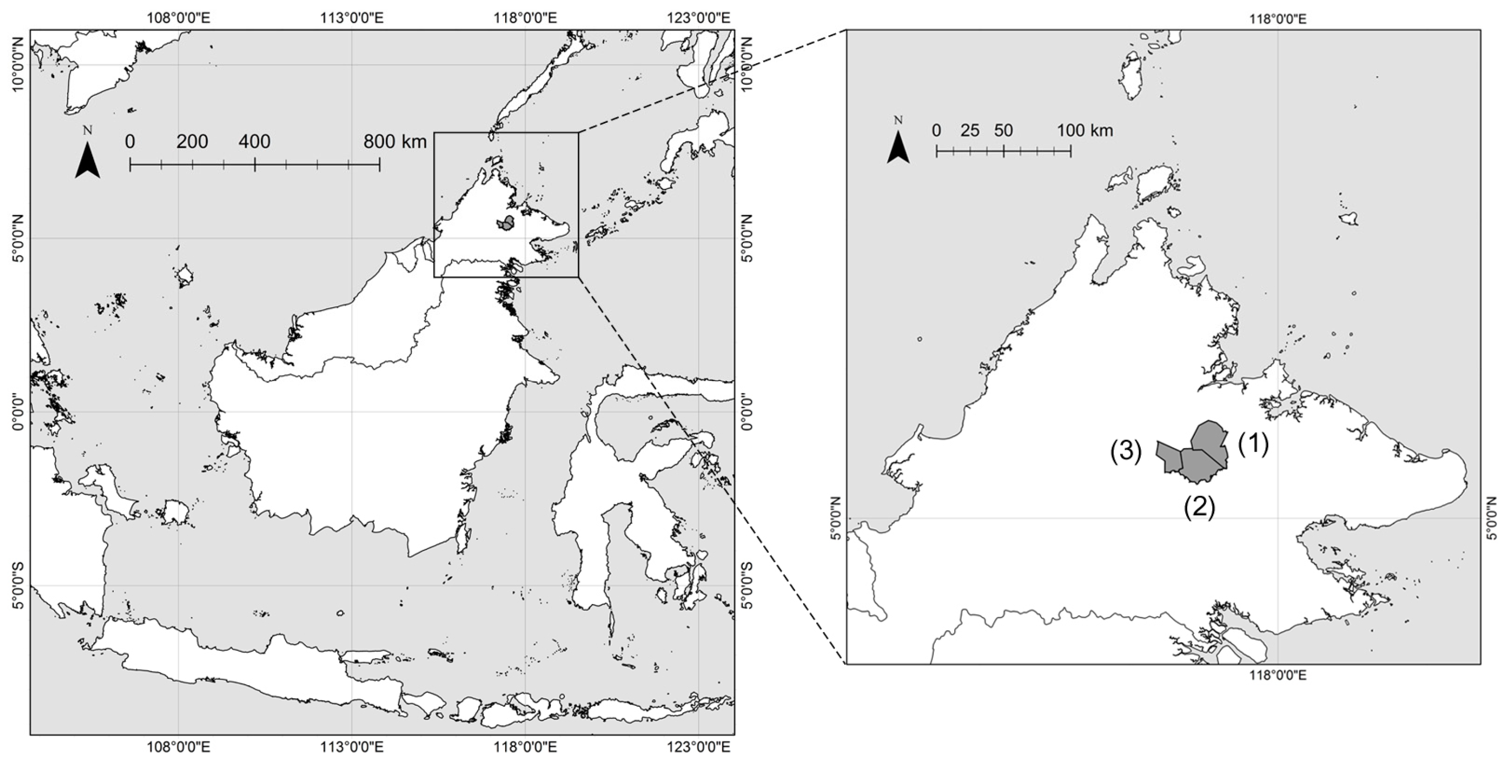
We collected data from the following forest management units (FMUs) in Sabah, Malaysia (
Figure 1): Deramakot FMU (5°14′–28′ N, 117°20′–38′ E, 551 km
2) and Tangkulap FMU (5°18′–31′ N, 117°11′–22′ E, 276 km
2). Supplementary data were also collected from Segaliud Lokan FMU (5°20′–27′ N, 117°23′–39′ E, 576 km
2). The three FMUs are adjacent to each other with the same undulating topography and the same equatorial tropical rain forest climate. Selective logging was a major driver of the changes of carbon stock and tree community composition in these forests. The elevation ranges from 12 m to 355 m. The original vegetation is a lowland dipterocarp rainforest throughout the three FMUs.
The areas of the three FMUs were initially logged in 1956, 1970 and 1958, respectively, using conventional logging methods (i.e., high-impact logging with no environmental considerations). In Deramakot, conventional logging continued until 1989, when all logging activities were halted for regrowth [
25]. Then, a long-term management plan with RIL was introduced to Deramakot in 1995. RIL is an improved method of selective logging, including pre-harvest inventory, mapping of all canopy trees, directional felling, liana cutting, and planning of skid trails, log decks, and roads [
26]. In combination with reduced-impact logging, a longer cutting cycle (i.e., 40 years) was strictly adhered to in accordance with the long-term management plan. These combined approaches helped to preserve forest intactness [
24,
27]. Deramakot was the first tropical forest certified by the FSC in 1997, and was considered a model of sustainable forest management by the Sabah Government [
25,
26]. Reflecting this logging history, we observed that the forests inside the Deramakot FMU were less disturbed based on aboveground biomass and various biological communities [
27]. In contrast, Tangkulap was repeatedly logged using conventional logging until 2003 and all logging activities were suspended thereafter. Tangkulap was entirely designated as a conservation forest in 2008 and later also certified by the FSC in recognition of its conservation-oriented long-term management plan in 2011. Both Deramakot and Tangkulap are currently managed directly by the Sabah Forestry Department. By contrast, Segaliud Lokan was repeatedly logged using conventional logging until 2002, after which RIL was implemented by the KTS Plantation Corp. Several areas were converted to plantation forests. It is currently certified by the Malaysian Timber Certification Council (MTCC).
In the following analysis, we compare spatiotemporal changes of ecosystem services, including carbon stock and forest intactness, between Deramakot and Tangkulap. A comparison of these two FMUs may elucidate differences between their respective spatiotemporal patterns in ecosystem services, reflecting the difference in past logging intensity, despite the fact that they are now both FSC-certified. We excluded Segaliud Lokan from this comparison because BOLEH was designed primarily for natural forests. The occurrence of plantation forests in Segaliud Lokan would interfere with the analysis. However, we included natural-forest data of Segaliud Lokan for the following remote-sensing analysis to enhance data points and statistical reliance.
2.2. Field Sampling
A total of 50 circular plots (20-m radius with 0.126 ha area each) were placed in the FMUs from December 2011 until May 2012 (hereafter 2012 inventory). Plots were placed with a stratified random design to represent various forest statuses, ranging from a near pristine high-stock forest to a highly degraded low-stock forest.
Prior to the placement of plots, the entire area was stratified to 6 degradation strata, from primary forest (stratum 1) to highly degraded, open area without trees (stratum 6), with the aid of Landsat Thematic Mapper (TM) band-7 imagery (see Imai et al. [
21] for the detailed procedure). Imagery obtained in 2010 was used for the stratification procedure. Briefly, we radiometrically converted Landsat data into Top-of-the-Atmosphere (TOA) reflectance values. Illumination artifacts caused by heterogeneous topography were reduced following the sun-canopy-sensor (SCS) model using TOA values [
28]. Shuttle Radar Topography Mission (SRTM) data were employed to correct for illumination artifacts. After masking all non-forest pixels, band-7 values were categorized into 6 strata using a level slicing method. Subsequently, we randomly placed 10 plots in each stratum of the five strata, except for stratum 6. Stratum 6, which is devoid of forests, was not actually sampled. Therefore, we established a total of 50 plots in strata 1 through 5. The distance between any two plots was greater than 100 m in order to minimize spatial autocorrelation.
All trees with ≥10 cm in diameter at breast height (dbh) were measured in dbh and identified as genera (actually operationally to species) in each circular plot. Voucher specimens were collected from the trees that could not be identified in the field and later used for identification at the herbarium of the Forest Research Centre, Sandakan. A polyvinyl chloride (PVC) stake was driven into the ground at the center of each circular plot as a permanent marker, and the exact coordinates (latitude and longitude) above the stake were recorded by averaging for two hours using a portable Global Positioning System (GPS).
In August 2014, we repeated the same procedure to inventory the forests as of 2014 (hereafter 2014 inventory). This time, we placed a total of 88 20-m-radius circular plots again evenly in strata 1–5 (actually, some of the plots had a 30 m × 40 m rectangular shape with approximately the same area as the circular plot because we used these rectangular plots for another purpose). None of the 88 plots overlapped with the 2012 plots because random sampling was deployed. In reality, a total of 50 plots would have been sufficient to derive reliable values of carbon stock and forest intactness according to our standard protocol manuals; however, we added 38 more plots that were placed for another research purpose to enhance model accuracy.
2.3. Pre-Processing of Satellite Images
We used the following two Landsat images to elucidate the temporal changes of carbon and forest intactness between 2009 and 2014 at the landscape level:
The raw digital numbers of each image were converted into top-of-atmosphere radiance. Subsequently, top-of-atmosphere radiance was converted to surface reflectance to compensate for atmospheric scattering and absorption effects using an atmospheric correction algorithm based on the Second Simulation of a Satellite Signal in the Solar Spectrum radiative transfer code (version. 1.1, [
29,
30]). The topographic effects on illumination were removed using the method described in Ekstrand [
31] with Shuttle Radar Topography Mission (SRTM) data. Finally, pixels covered with clouds/shadow were removed according to the procedure described in Fujiki et al. [
22]; pixels covered/affected by cloud/shadow were clustered as segments based on a homogeneity criterion with eCognition Developer 8.7 and all segments above a certain threshold were removed as cloud/shadow. Removed segments were filled in using the cloud-free areas of temporally adjoining data. Calibrated cloud-free parts of adjoining secondary images were incorporated into the missing parts of the base image (see Fujiki et al. [
22] for the details). We used ERDAS Imagine version.11.0 and ArcGIS 9.3.1 for these pre-processing procedures.
2.4. Estimating Spatiotemporal Changes of Carbon Stock
Above-ground biomass (AGB) of each plot was estimated according to the allometric equation obtained by Chave et al. [
32] as:
where D is dbh (cm) and ρ is the wood-specific gravity (g/cm
3). We obtained the wood-specific gravity ρ for the sampled species/genera from various sources (see Imai et al. [
21] for the detailed procedure). We estimated AGB of each plot for both the 2012 and 2014 inventories. Subsequently, the estimated AGB of each plot was multiplied by 0.48 to derive the amount of carbon.
A multivariate regression model was established with the amount of carbon per plot as a dependent variable and reflectance of the corresponding pixel on a Landsat image as an independent variable. Here, textural metrics of the 3 × 3 pixels surrounding each plot were also added as independent variables. The amounts of carbon derived from the 2012 inventory were regressed with the reflectance and textural metrics of the 2009 Landsat imagery (Landsat TM, Path117/Row56, 11 August 2009). The amounts of carbon derived from the 2014 inventory were regressed with the reflectance and textural metrics of the 2014 Landsat imagery (Landsat OLI, Path117/Row56, 06 June 2014). The 2012 inventory data were regressed with the 2009 Landsat imagery without correcting for the tree growth between 2009 and 2012 for a first approximation of the 2009 condition because there were neither 2009 inventory data nor clear 2012 Landsat images; this was logical because all plots measured in 2012 were also present in 2009. However, modeling using the 2012 inventory data without the correction for tree growth would slightly overestimate the modeled 2009 carbon stock.
The following Landsat metrics were used as independent variables: reflectance value of each band (Band1TM/OLI, Band2TM/OLI, Band3TM/OLI, Band4TM/OLI, Band5TM/OLI, Band6OLI, Band7TM/OLI), NDVI [
33], normalized difference water index (NDWI) [
34,
35], normalized difference soil index (NDSI) [
36], and enhanced vegetation index (EVI) [
37]. We calculated mean value of each Landsat metric within a 20-m radius from the center of a plot to represent the plot. The normalized indices were calculated as follows:
In addition, we used the following metrics as proxies for spectral heterogeneity because degradation of forest canopies might affect the heterogeneity of the spectral pattern: the coefficient of variation (CV), standard deviation (SD), and textures of the gray-level co-occurrence matrix (GLCM) [
38]. CV, SD, and textures of the GLCM were derived using a 3 × 3 pixel window based on the reflectance values and each of the normalized indices. GLCM is a tabulation explaining how often different combinations of gray levels occur at a specified distance and orientation in an image object [
39]. Homogeneity, contrast, angular second moment, entropy, dissimilarity, correlation, mean, and standard deviation were derived as the indices of the textures. Overall, 120 and 132 metrics were generated based on Landsat TM and OLI, respectively. For developing an adequate regression model, independent variables were selected using a stepwise selection from the full model containing all metrics to avoid multi-collinearity among the independent variables. We did not find significant multi-collinearity because the variance inflation factor (VIF) of selected independent variables, which is an indicator of multi-collinearity, was in all cases less than 10. Established models are shown in
Table 1. Subsequently, each of the models (2009 and 2014 models) was extrapolated to the entire area to estimate the amount of carbon outside the inventory plots based on the 2009 or 2014 Landsat imagery.
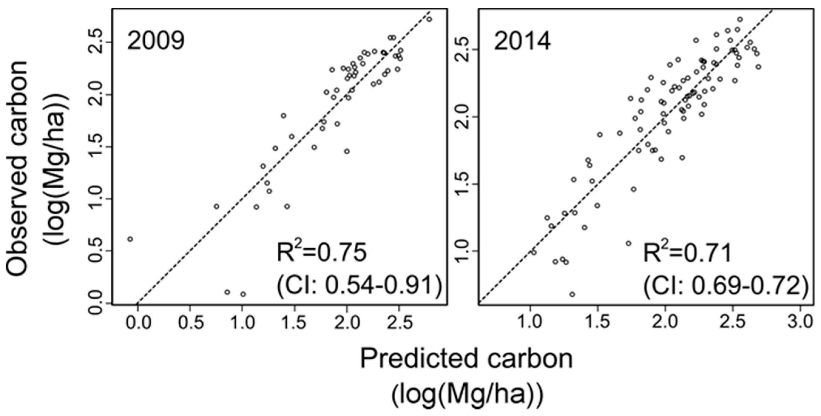
We took a Monte Carlo approach to show model accuracy and to test for significant differences of mean AGB values between 2009 and 2014 for a given FMU, or between FMUs for a given year (2009 or 2014). Four-fifths of the plots in each stratum (e.g., a total of 40 plots in the case of 2009, and 70 plots in 2014) were randomly selected to construct the AGB models for 2009 and 2014, respectively. The model predictions for AGB of the remaining one-fifth of the plots were regressed with the observed values both for 2009 and 2014, and the adjusted R
2 values were determined. Based on these models, we estimated the mean AGB value each for Deramakot and Tangkulap each in 2009 and 2014. These steps were reiterated 1000 times for 2009 and 2014, respectively, to derive the 95% confidence intervals (CIs) of the adjusted R
2 and the mean AGB values. The statistical tests were conducted using R ver. 3.20 [
40].
2.5. Estimating Spatiotemporal Changes of Forest Intactness
It has been well established that tree-species/genus composition is one of the best indexes of the magnitude of forest degradation [
21,
23,
27]. Similarity of the species/genus composition of a given forest with that of pristine forests decreases linearly with increasing magnitude of degradation of the forest [
21,
27]. We applied this principle to the forests of Deramakot and Tangkulap and evaluated the status of a given forest in terms of its compositional similarity with pristine forests [
21]. The compositional similarity with pristine forests is termed here “forest intactness” and can be mapped through a special extrapolation procedure [
22]. Here, we compared generic composition among plots instead of species composition because logging causes similar shifts in generic composition as in species composition [
21,
23]. The procedure of mapping “forest intactness” for a given time has been described by Fujiki et al. [
22]. We elaborate here on the procedure to elucidate temporal changes of “forest intactness”.
Firstly, differences in community composition among these plots laid out for estimating carbon storage were examined by using an ordination technique. We used a composite of the data of both the 2012 and 2014 inventories to derive a single data matrix to allow for a comparison between these two years using standardized scores. The Chao distance [
41] and the number of trees of each genus were used to calculate a distance matrix. An ordination of plots was conducted with non-metric multidimensional scaling (nMDS) using the “metaMDS” procedure in the Vegan package in R [
42].
Although plots were located distantly from each other, we could not completely rule out the possibility of spatial autocorrelations among plots. Therefore, we tested autocorrelations among plots, but did not find significant effects of spatial autocorrelations (see
Figure S1,
Supplementary Materials).
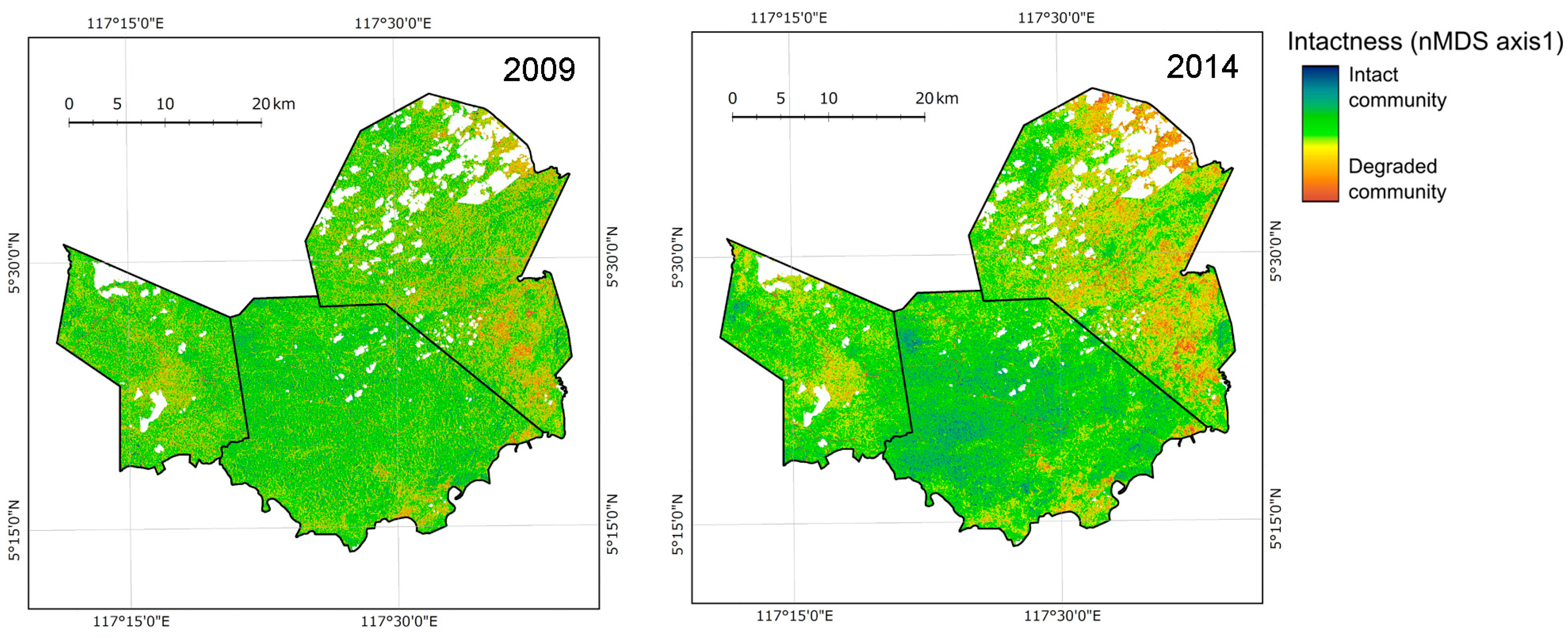
A multivariate regression model was established with the derived nMDS axis-1 scores of plots as dependent variables, and reflectance and textural metrics of the corresponding pixels on a Landsat image as independent variables; the nMDS axis-1 scores of the 2012 inventory plots were regressed with the 2009 Landsat TM imagery and those from the 2014 inventory were regressed with the 2014 Landsat OLI imagery, as was conducted for the carbon analysis. We did not correct the nMDS axis-1 scores of 2012 when regressed with the 2009 imagery because the tree growth during 3 years between 2009 and 2012 would not substantially change tree-species composition. We used the same Landsat metrics as a carbon stock estimate in this analysis. Established models are indicated in
Table 2. Each model was extrapolated to the entire area on the 2009 and 2014 Landsat imagery, respectively. This procedure yielded the maps of forest intactness for 2009 and 2014.
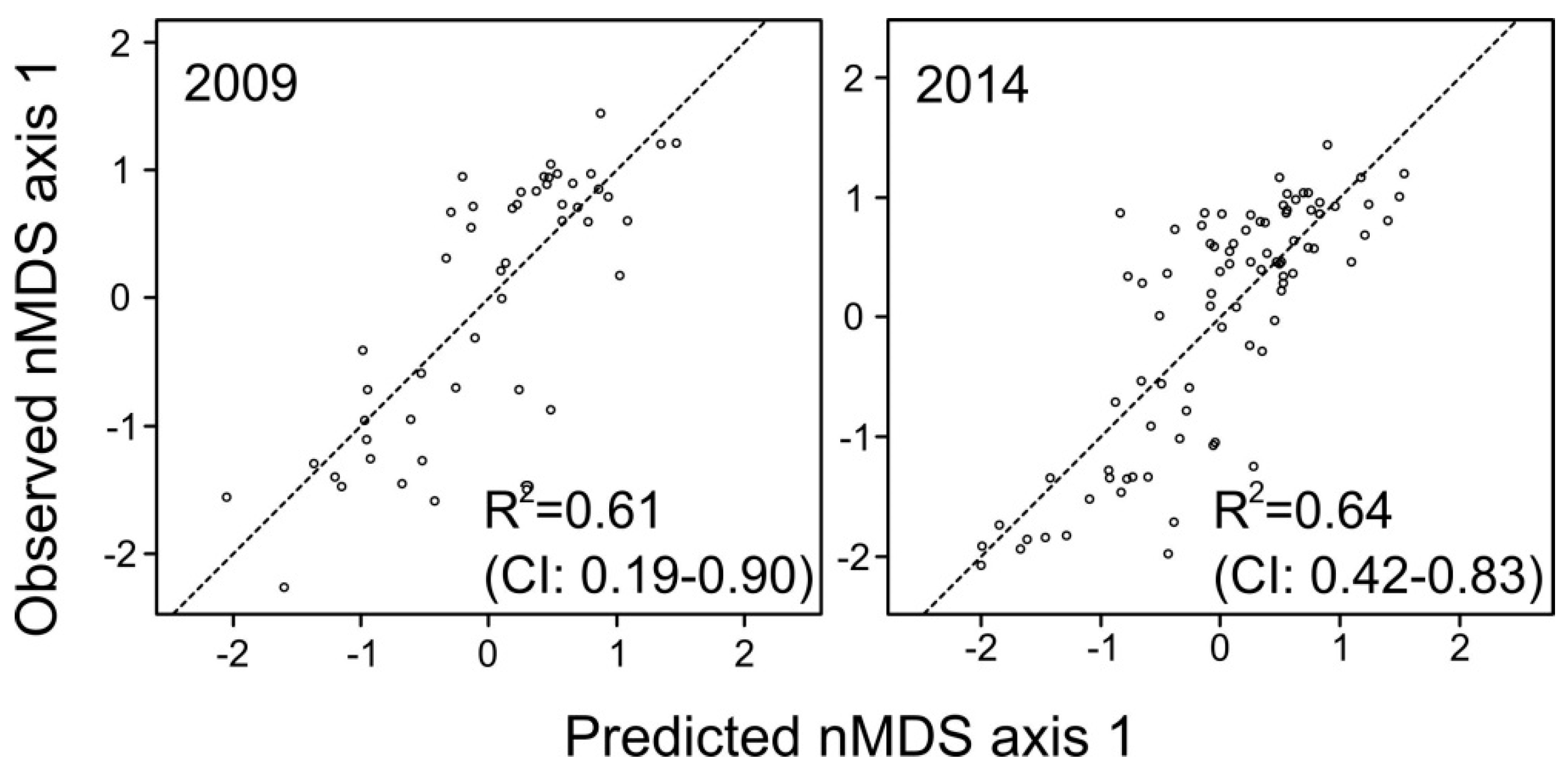
We also took a Monte Carlo approach to test significant differences of mean nMDS axis-1 scores between 2009 and 2014 for a given FMU, or between FMUs for a given year (2009 or 2014) [
22]. Four-fifths of the plots in each stratum were randomly selected to construct the 2009 and 2014 model, respectively. Based on these models, we estimated mean nMDS axis-1 scores for Deramakot and for Tangkulap in 2009 and in 2014. The model predictions for nMDS axis-1 scores of the remaining one-fifths of the plots were regressed with the observed values both for 2009 and 2014, and the adjusted R
2 values were collected. Based on these models, we estimated mean nMDS axis-1 scores for Deramakot and for Tangkulap in 2009 and in 2014. These steps were reiterated 1000 times each for 2009 and 2014 to derive the 95% CIs of the adjusted R
2 and the mean reiterated nMDS axis-1 scores. The statistical tests were conducted using R ver. 3.20 [
40].
4. Discussion
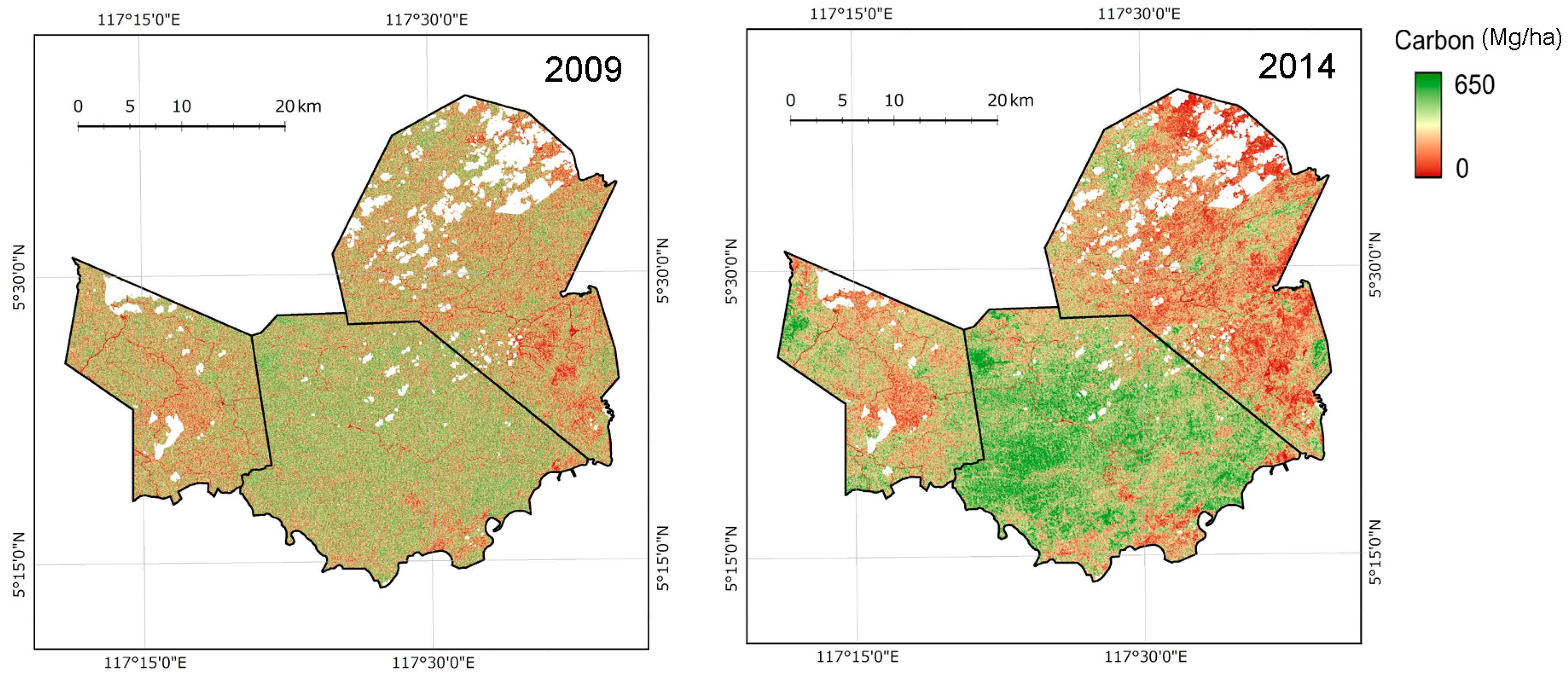
The BOLEH method successfully elucidated the spatiotemporal changes of carbon density and forest intactness as maps across the three FMUs between 2009 and 2014. The procedure to map forest intactness was already well described by Fujiki et al. [
22], who demonstrated forest intactness maps of six FMUs across Borneo. They demonstrated that the mean values of and the frequency distributions of forest intactness significantly differed among FMUs, reflecting the forest management schemes. Our current study further demonstrates that the BOLEH method is useful to monitor temporal changes of forest intactness in a given FMU. Particularly, our BOLEH method could reveal a significant increase of mean carbon density value and a marginally significant increase of mean forest intactness value in Deramakot between August 2009 and June 2014 (time of acquisition of Landsat data) in spite of the continued production of timber. Deramakot FMU produced a total of 43,023 m
3 volume of round logs in two compartments during the corresponding five years. The increases in both mean carbon density and forest intactness suggest that the regrowth in fallow compartments outweighed the harvest. Our BOLEH method based on landscape analysis could successfully evaluate such a balance between negative impacts of harvesting and positive impacts of leaving areas fallow.
Co-benefits of sustainable forestry with RIL on the carbon storage function have already been suggested by Imai et al. [
24], Langner et al. [
43] and Langner et al. [
44], who compared Deramakot with Tangkulap with a snapshot of carbon density in a given year using a space-for-time approach. In our current analysis, we have directly proved the co-benefits of sustainable forestry and RIL on the carbon storage and forest intactness by continuous monitoring. The vast majority of production forests across Malaysia and Indonesia in Borneo have been mildly to highly degraded due to past multiple entries of logging. Deramakot is not an exception. The mean annual harvest with RIL from such degraded secondary forests is 30 m
3/ha and the mean annual harvest area is 347 ha over the 20 years between 1995 and 2016 in Deramakot (unpublished statistical data). Collateral damages are also unavoidable even if timber is carefully harvested under RIL. If we assume that harvest practices with collateral damage produce 30 m
3/ha of waste (i.e., equivalent to the harvested volume), a total of 60 m
3/ha of trees are removed annually from 347 ha, giving rise to a total removal of 20,820 m
3/year (or 10,410 tons carbon/year in Deramakot assuming that 1 m
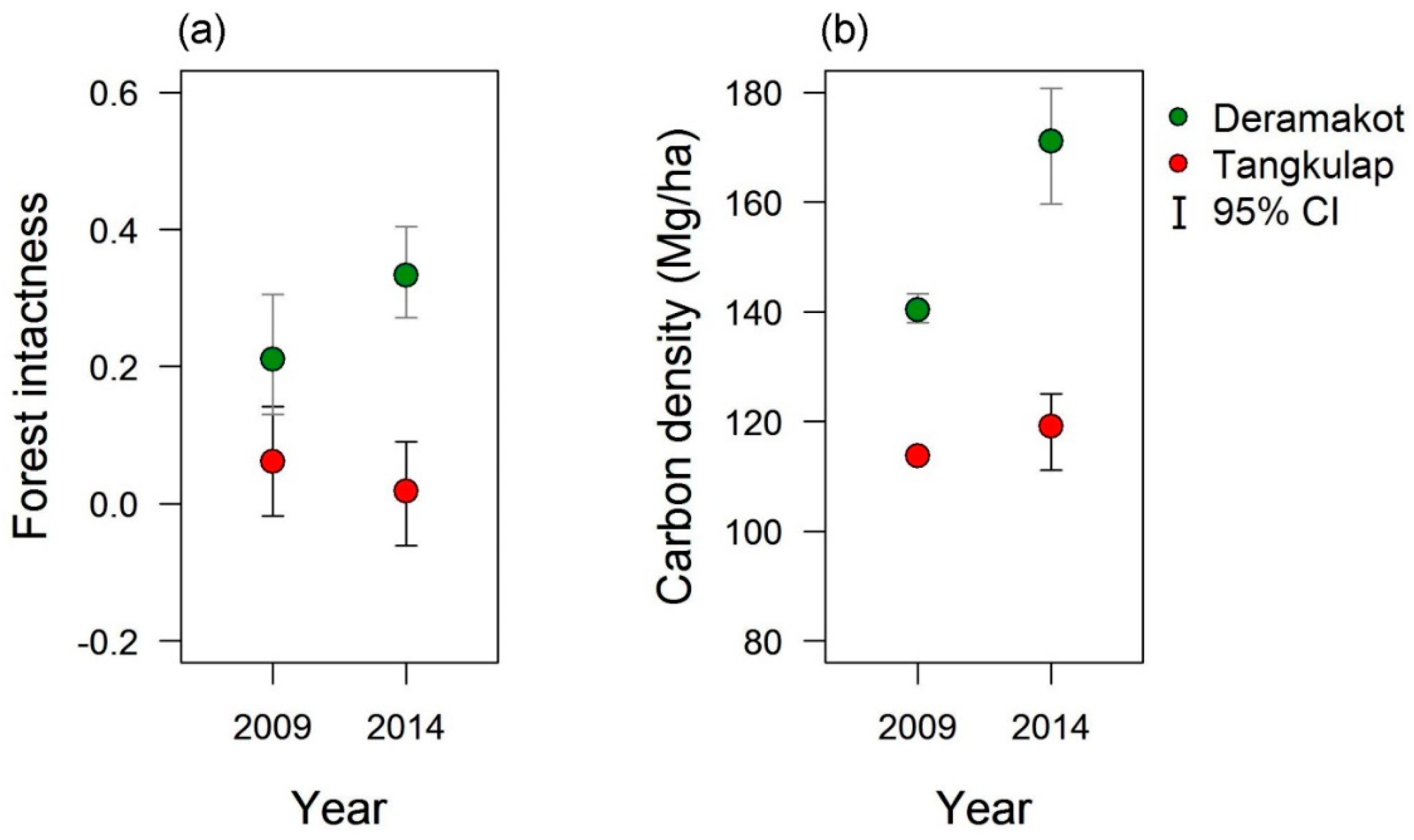
3 volume is equivalent to 0.5 ton carbon). On the other hand, there are a total of approximately 54,653 ha of fallow compartments each year in Deramakot. Tree regrowth with an increment of merely 0.19 ton carbon/ha/year will make up for the removed carbon of 10,410 tons. Our results indicate that mean carbon density significantly increased from 140 (133–151) ton/ha to 170 (162–179) ton/ha during 5 years from 2009 to 2014, which is equivalent to 6 tons carbon/ha/year including harvested compartments. The ratio of mean harvest area to the fallow area is 347 ha to 54,653 ha, and this wide ratio (i.e., a long rotation) is important to sustain the surplus in carbon budget in secondary production forests. Therefore, Bornean tropical production forests with a comparable biomass stock and a comparable management plan (a long rotation period and moderate harvesting) to those of Deramakot will likely be assured of an increase of carbon stock.
On the other hand, mean forest intactness only marginally increased between 2009 and 2014 in Deramakot, as indicated by the fact that the 95% CIs overlapped slightly between these years. Why did the mean forest intactness not significantly increase while the mean carbon density significantly increased during the same period? Probably, a longer time is required for tree communities to recover in species/genus composition, while carbon increments can occur as a simple function of time. There must be a shift of tree communities (from pioneer to climax species) in order to demonstrate a significant increase of forest intactness. For instance, a vast area of young pioneer -tree stands will support a rapid carbon increment but not an increment in forest intactness because species composition is rather stabilized in such stands. Therefore, monitoring of both ecosystem services (carbon and forest intactness) is necessary for the meaningful evaluation of ecosystem integrity/health.
Why the mean carbon density and forest intactness did not increase in Tangkulap between 2009 and 2014 in spite of the suspension of logging operations is an intriguing question. As reported by Kitayama [
27], the natural forests of Tangkulap have been highly degraded by past repeated logging; they are currently dominated by stands of pioneer trees such as
Macaranga or by fern grasslands. The shift from such pioneer stands to climax stands will be extremely slow. On the other hand, the slow recovery of carbon stock is puzzling because the building phase of secondary succession is known to accumulate carbon at a rapid rate. Poorter et al. [
45] reported a median carbon accumulation rate of 3.05 ton-C/ha/year in secondary forests at 20-year age in the Neotropics. Our estimate of the carbon accumulation rate in Tangkulap is merely 0.8 ton-C/ha/year, although this value was not statistically significant. Probably, the occurrence of vast, thick fern stands is related to the slow recovery because the regeneration in such thick fern stands is extremely slow [
46]. When forest regrowth is analyzed, such fern stands tend to be avoided for sampling by ecologists. Moreover, mean tree mortality may be greater in senescent pioneer-tree stands (Imai, personal observation). Therefore, landscape-level evaluations based on remotely sensed data like our BOLEH are required to elucidate the spatially and temporally explicit patterns of carbon (and forest intactness). Another possible reason for the slow carbon accumulation in Tangkulap could be the use of the 2012 inventory data for developing the 2009 carbon model without correcting for the tree growth between 2009 and 2012, because this would slightly overestimate the carbon density for 2009. However, this would not be an important weakness of our study, because our major objectives here were to test our algorithms, but not to investigate the carbon dynamics
per se.
The FSC ecosystem-services certification has set forth a standard by which forest managers must verify at least the non-existence of net negative management impacts on ecosystem services [
12]. The 5-year period seems to be adequate for verifying that there are no net negative management impacts on carbon density or forest intactness using our BOLEH in the case of Deramakot. However, in an FMU where the harvested volume outweighs regrowth (i.e., net negative impacts), the 5-year period may not be long enough to demonstrate a statistically significant negative impact (i.e., reduction in mean values of carbon and forest intactness) because 95% CIs tend to be fairly wide in our method. Fujiki et al. [
22] discussed the reasons for wide CIs and suggested that the number of plots was too small for cross-validation. When outlier plots are used to develop a model (to explain carbon or forest intactness with Landsat metrics), residuals become large, giving rise to disproportionately large or small mean values; this must be the case for the very low coefficient of correlation (i.e., 0.19) in the 2009 nMDS cross-validation. The coefficient of correlation for the lower 95% CI in the 2014 nMDS cross-validation was relatively high (i.e., 0.42) probably because we used a total of 86 plots. Here, we still suggest using a total of 50 plots as standard sampling for reducing field efforts. If we maintain this standard sampling procedure, wide 95% CIs will be inherent to our methods. Therefore, forest managers should use our method only when mean values of carbon and forest intactness tend to increase or to be stable in order to verify the non-existence of net negative impacts for the FSC ecosystem-services certification. The 5-year period is equivalent to one period of an FSC forest certification. If BOLEH is incorporated into the assessment procedures of the regular FSC certification for sustainable management, forest managers can verify the enhancement of ecosystem services with low cost in addition to criteria pertinent to environmental values and impacts (principle 6) and monitoring and assessment (principle 8). It should be noted, however, that forest intactness cannot be used as a surrogate of richness of biological taxa because compositional distances from a pristine forest are unrelated to richness of biological taxa [
21,
27].

 ,
, 


