Spatio-Temporal Variation Analysis of Landscape Pattern Response to Land Use Change from 1985 to 2015 in Xuzhou City, China


1
School of Resources and Geosciences, China University of Mining and Technology, Xuzhou 221116, China
2
School of Spatial Planning, TU Dortmund, 44227 Dortmund, Germany
*
Author to whom correspondence should be addressed.
Sustainability 2018, 10(11), 4287; https://doi.org/10.3390/su10114287
Submission received: 27 September 2018
/
Revised: 15 November 2018
/
Accepted: 15 November 2018
/
Published: 19 November 2018
(This article belongs to the Special Issue Spatial Analysis of Urbanization towards Urban Sustainability)
Abstract
:Rapid urbanization has dramatically spurred economic development since the 1980s, especially in China, but has had negative impacts on natural resources since it is an irreversible process. Thus, timely monitoring and quantitative analysis of the changes in land use over time and identification of landscape pattern variation related to growth modes in different periods are essential. This study aimed to inspect spatiotemporal characteristics of landscape pattern responses to land use changes in Xuzhou, China durfing the period of 1985–2015. In this context, we propose a new spectral index, called the Normalized Difference Enhanced Urban Index (NDEUI), which combines Nighttime light from the Defense Meteorological Satellite Program/Operational Linescan System with annual maximum Enhanced Vegetation Index to reduce the detection confusion between urban areas and barren land. The NDEUI-assisted random forests algorithm was implemented to obtain the land use/land cover maps of Xuzhou in 1985, 1995, 2005, and 2015, respectively. Four different periods (1985–1995, 1995–2005, 2005–2015, and 1985–2015) were chosen for the change analysis of land use and landscape patterns. The results indicate that the urban area has increased by about 30.65%, 10.54%, 68.77%, and 143.75% during the four periods at the main expense of agricultural land, respectively. The spatial trend maps revealed that continuous transition from other land use types into urban land has occurred in a dual-core development mode throughout the urbanization process. We quantified the patch complexity, aggregation, connectivity, and diversity of the landscape, employing a number of landscape metrics to represent the changes in landscape patterns at both the class and landscape levels. The results show that with respect to the four aspects of landscape patterns, there were considerable differences among the four years, mainly owing to the increasing dominance of urbanized land. Spatiotemporal variation in landscape patterns was examined based on 900 × 900 m sub-grids. Combined with the land use changes and spatiotemporal variations in landscape patterns, urban growth mainly occurred in a leapfrog mode along both sides of the roads during the period of 1985 to 1995, and then shifted into edge-expansion mode during the period of 1995 to 2005, and the edge-expansion and leapfrog modes coexisted in the period from 2005 to 2015. The high value spatiotemporal information generated using remote sensing and geographic information system in this study could assist urban planners and policymakers to better understand urban dynamics and evaluate their spatiotemporal and environmental impacts at the local level to enable sustainable urban planning in the future.
1. Introduction
In China, significant economic development has resulted in the rapid expansion of urban areas in cities since the 1980s, placing tremendous stress on the environment, natural resources, and public health [1,2,3,4]. Dynamic change monitoring and quantifying of urban areas play a critical role in studying urban growth modeling [5,6], urban heat islands [7,8], and land cover changes [9,10,11]. Accurate and long-term monitoring of urban dynamics is essential for understanding and regulating the consequences of urbanization at regular intervals [2]. Therefore, urban expansion has increasingly become a major issue facing many fast-developing cities experiencing a sharp growth in urban population and intensive human activities [5,12].
Remote sensing provides a useful tool for monitoring and quantifying land use/land cover (LULC) changes at high spatial resolution and annual temporal scales, to systematically track the magnitude and spatial trends of urbanization [2,5,13]. Several LULC datasets have been developed using remote sensing, such as the 500-m Moderate-Resolution Imaging Spectroradiometer Global Yearly Land Cover Type (MCD12Q1, from 2001 to 2013) [14], 30-m National Land Cover Database (NLCD, 1992, 2001, 2006, and 2011) [15], and the 30-m Finer Resolution Observation and Monitoring-Global Land Cover (GLOBELAND30, 2000 and 2010) [16]. However, these datasets are either not accurate enough for city-level research or lack sufficient temporal resolution, and are hard to use to characterize the urban long-term spatial-temporal dynamics [17,18,19]. Thus, various approaches have been proposed to derive urban land from different remote sensing images, such as spectral mixture analysis [20,21], object-based approaches [22,23], and a multivariate texture approach [1]. In addition, Since the optical spectrum of urban land is complex and can be confused with bare and fallow land, accurate urban land extraction is extremely difficult utilizing single-sensor data [24]. Various indices have been used to distinguish urban land from other land, such as the multi-source Normalized Difference Impervious Surface Index (MNDISI) [25], the Biophysical Composition Index (BCI) [26], the Enhanced Built-Up and Bareness Index (EBBI) [27], Normalized Difference Urban Index (NDUI) [24], and the Normalized Difference Bareness Index (NDBaI) [28]. For instance, MNDISI is used to highlight urban areas combining Landsat surface temperature and fine-resolution International Space Station night light images [24,25]. However, temperature varies dramatically along with terrain changes.
To track multi-temporal trajectories of urban areas, change detection techniques have been widely employed for comparison of paired images. The most common methods include image differencing, principal component analysis, and post-classification comparison [29]. Note that no single approach is optimal and applicable to all cases [30]. The Landsat series data (Thematic Mapper, TM; Enhanced Thematic Mapper plus, ETM+; and Operational Land Imager, OLI) are useful for change detection due to their high temporal-spatial resolution and spectral resolution [31]. Reynolds et al. [2] presented a temporal trajectory polishing method to generate high frequency, high accuracy, and consistent trajectories of urban land-cover change in Northwest Arkansas. Son et al. [32] explored urban growth using the linear mixture model in Ho Chi Minh City, Vietnam through Landsat images. Villa [33] proposed the Soil and Vegetation Index (SVI) and used the multi-temporal SVI ratios threshold for identifying urban growth areas.
Understanding the dynamic changes in landscape patterns is critical for revealing the process of urbanization and its impacts on the environment [12,34,35]. In this context, identifying the driving forces contributes to protecting and properly planning landscapes with high value that are located close to big cities [36]. Landscape metrics have been widely used to quantify landscape patterns and analyze the dynamic changes in the regional landscape [37]. Liu and Yang [38] utilized landscape metrics to characterize land use changes and reveal the underlying processes of urban sprawl. The landscape change index (LCI) was proposed to assess the level of change in different periods [39]. Due to spatial heterogeneity, landscape patterns changes can be used to indicate the spatial distribution of urbanization modes [34]. Based on spatial variation analysis of landscape patterns and related built-up growth, Yang et al. [12] evaluated and modeled the relationship between the urban sprawl characters and landscape pattern based on different temporal scales.
In this study, to highlight urban areas, we employed medium-resolution Landsat and coarse-resolution Defense Meteorological Satellite Program/Operational Linescan System (DMSP/OLS) nighttime light (NTL) data as both have long historical archives. There are two key issues we wanted to address. Firstly, we derived the maximum Enhanced Vegetation Index (EVI) of each pixel from the Landsat 32-day EVI Composites and generated the annual “Max EVI” composite to distinguish between urban land and fallow land. Secondly, we constructed and calculated the Normalized Difference Enhanced Urban Index (NDEUI) combining the Max EVI composite with normalized NTL data for each year, which distinguishes between the urban area and bare or fallow land. Then, random forest (RF) was employed as a basic classifier to obtain annual classification result based on the original spectral bands, as well as NDNEI. All the above were implemented on the Google Earth Engine (GEE), which is a cloud computing platform. This study aimed to monitor and reveal land use change and urban spatial expansion patterns in Xuzhou, China from 1985 to 2015. The landscape patterns were analyzed at the class and landscape levels to understand the process of urbanization and its impacts on the environment. In this context, it was essential to develop a systematic approach including both spatiotemporal monitoring and landscape pattern analysis. Finally, we quantified the LULC changes, landscape pattern, and analysis trends of urban sprawl in Xuzhou from 1985 to 2015.
2. Material and Methodology
2.1. Study Area
Xuzhou (33°43′–34°58′ N, 116°22′–118°40′ E) is located in the northwest of Jiangsu Province, China, adjacent to Shandong, Henan, and Anhui provinces (Figure 1). Xuzhou is about 300 km away from Nanjing, Jinan, Zhengzhou, and Hefei, the capitals of adjacent provinces. It is also the main city of the Huaihai Economic Zone, which has an area of 17.6 million km2 and a population of 120 million. Xuzhou is the largest city among the adjacent 19 cities, consisting of 5 administrative districts, 3 counties, and 2 county-level cities. It is mostly comprised of plains, with small areas of hillocks and mountains in the central and eastern regions. The Old Yellow River flows across the city generally in a west to southeast direction, and the Yunlong Lake is located in the south part of the region. For the purposes of this study, the central area of the city was selected, which is composed of four districts: Quanshsn, Gulou, Yunlong, and Jiawang. The central area covers 1058 km2. Since the 1980s, Xuzhou has experienced significant economic growth and rapid urbanization. The urban population increased from 0.67 million in 1978 to approximately 2.02 million in 2015. The gross domestic product (GDP) has increased to 531.952 billion RMB Yuan in 2015 from 2.14 billion in 1978 (Figure 2).
2.2. Data and Preprocessing
The analyses of land use changes and landscape pattern were conducted based on a post-classification change detection strategy. The procedural workflow proposed in this study is illustrated in Figure 3. Each component will be described in detail, including data sources and pre-processing, classification scheme, and land use change and landscape pattern analysis.
2.2.1. Landsat Time Series
With free access to the Landsat archive and other new remote sensing data sources online, it is possible to exploit multi-temporal remote sensing data to map urban changes. Google Earth Engine is a cloud-based platform for planetary-scale environmental data analysis integrating a petabyte-scale archive of publicly available remotely sensed imagery and other data. Landsat series Top-of-Atmosphere (TOA) reflectance data (orthorectified) were used in this study, including Landsat TM, ETM+, and Landsat OLI. The data were produced from Level L1T orthorectified scenes, using the computed TOA reflectance [40]. These composites were created from all scenes from each 32-day period beginning from the first day of the year and continuing to the 352nd day of the year. The last composite of the year, beginning on day 353, overlapped the first composite of the following year by 20 days [2]. All the images from each 32-day period were included in the composite, with the most recent pixel as the composite value.
To avoid confusion between new urban land and other land cover types (such as bare land, or fallow or post-harvest cropland), we combined images from multiple seasons (Figure 4). There is a high probability that bare or cropland is vegetated during at least one season of each year, and thus can be separated from built-up areas that are predominantly non-vegetated all year-round. However, it is unrealistic to select all the seasonal images in a year.
Apart from the raw data or preprocessing data, Google Earth Engine also provides all kinds of composite products derived from raw data, such as 32-day composites for NDWI, NDVI, and EVI. In this study, we compared the 32-day NDVI composite with the EVI composite (Figure 5). For EVI, it is clear that all the land use types have better separability, especially in summer (Figure 5). For crop land and grassland, EVI has a higher value than the corresponding NDVI, with the maximum value being 1. The statistical analysis results also indicate that EVIMax has a better variation and dispersion than NDVIMax for different land-use types. Thus, the EVI was employed in this study, which is generated from the near-infrared (NIR), red, and blue bands of each scene, and it ranges in value from −1.0 to 1.0 [41] as shown in Equation (1).
where , , and are the TOA reflectance of blue, red, and NIR bands for Landsat series imagery.
2.2.2. DMSP/OLS NTL Data
The version 4 DMSP/OLS NTL data with 30 arc second (about 1 km) resolution can also be obtained from the Google Earth Engine platform [42]. It has the unique capability to detect visible and near-infrared (VNIR) emission sources at night. Each image in the collection contains 4 bands: avg_vis, cf_cvg, avg_lights_x_pct, and stable_lights. The cleaned up avg_vis (stable_lights) was selected in our study, as it contains the lights from cities, towns, and other sites with persistent lighting, including gas flares. Ephemeral events, such as fires, were discarded. The background noise was identified and replaced with values of zero. The DN values were recorded in the range of 0 to 63.
2.2.3. Data Pre-Processing
The 32-day EVI composites precede the NDVI composites in distinguishing among the different land use types (Figure 5). Thus, 32-day EVI composites were used in this study. Due to growth cycles and the seasonality of crops, it is difficult to determine the optimal TOA reflectance data for each year, which are also affected by the clouds. Thus, in order to overcome these limitations, one effective approach involves generating a maximum EVI image from multi-temporal EVI images. In this study, 32-day EVI composites were selected for each year, which included 12 EVI images. For each pixel, we obtained the maximum EVI over the year and generated the EVImax imagery for each year. Another important role for the EVImax imagery is removing the impacts of cloud. Therefore, the final EVImax imagery is cloud-free with a data range between −1 and 1.
Due to the lack of on-board calibration and the differences between sensors, there are systematic biases in NTL data. Consequently, the individual composites of the NTL data had to be inter-calibrated carefully to generate a consistent NTL time series [43,44,45]. Pandey et al. [46] compared and evaluated the existing nine calibration methods to provide guidance on their relative strengths and weaknesses. Their research results showed that inter-calibration reduces systematic biases consistently across most countries using the methods adopted in reference [45] and reference [47]. Pandey et al. [46] obtained marginally better results than Elvidge et al. [45]. The coefficients for inter-calibration provided by Zhang et al. [47] were adopted in our study.
Notably, the calibrated DMSP/OLS NTL values are recorded in the range [0, 63], whereas EVI values are between −1 and 1. Here, we normalized the calibrated DMSP/OLS NTL into the range of [0, 1] to enable comparison. Then, we resampled the normalized data to 30 m resolution.
2.2.4. Normalized Difference Enhanced Urban Index (NDEUI)
DMSP/OLS NTL has been widely used to study urban sprawl, and several spectral indices have been proposed. Zhang et al. [48] proposed a new index, VANUI, combining MODIS NDVI and DMSP/OLS NTL. Zhang et al. [24] proposed the Normalized Difference Urban Index (NDUI) to obtain urban spatial structures on a much finer scale. However, each annual NDVI composite was generated from contiguous three-year ETM+ imageries, which confuses changed land use types during the three years, especially in rapidly developing regions. The thresholds of NDVI provided by the authors is not suitable for all cases. Cheng et al. [49] constructed the Biophysical Composition Index (BCI)-Assisted NTL Urban Index (BANI) based on the correlations between BCI and normalized DMSP/OLS NTL data. BCI was calculated using MODIS surface reflectance data, which not only included several complex steps, including Tasseled Cap transformation, but also only produced a coarse-resolution BCI. Thus, in our study, we combined the EVImax imagery mentioned in Section 2.2.1 with the 30 m resolution normalized DMSP/OLS NTL data to generate a new index, the Normalized Difference Enhanced Urban Index (NDEUI) calculated using Equation (2):
where NTL is the normalized DMSP-OLS stable nighttime lights data, and EVImax imagery is generated from the all the 32-day EVI composites for one year.
2.3. Classification with Random Forests
According to the definition by Schneider and Mertes [50], urban land is dominated by the built environment with more than 50% coverage ratio within a landscape unit, which includes all non-vegetative and human-constructed elements (building, roads, etc.). Thus, five land cover categories were classified from remote sensing imagery in this study: Urban land, water bodies, agriculture/grassland, forest, and barren land.
The annual classification was implemented using optimal Landsat TOA reflectance as the base scene and the corresponding NDEUI. Due to the seasonal phenology of the study area and cloud cover, a base scene with less cloud cover acquired from July to October was preferred. It should be noted that there were no DMSP/OLS NTL data before 1992 or after 2013. According to the Statistical Yearbook of Xuzhou City, there was no obvious urban land change during the two periods. Thus, the DMSP/OLS NTL data were replaced by the data of 1992 and 2013 for annual classification before 1992 and after 2013, respectively.
To reduce possible biases caused by training samples and to obtain relative classifiers, a hierarchical sampling scheme [5] was adopted in our study. Firstly, with the support of EVImax imagery in 2005 and Google Earth, training samples were collected on the cloud-based platform (Google Earth Engine). The training samples were loaded as the initial training samples of a specific temporally adjacent year, and were rechecked to identify whether their types had changed. We could reassign their types, move to corresponding positions, or delete the changed samples. Thus, we repeated the procedure and obtained all the training samples for all years.
RF is an ensemble learning method for classification, regression, and other tasks [51] that uses trees as base classifiers. RF is a combination of many classifiers and confers some special characteristics [52]. RF increases the diversity of the trees by making them grow from different training data subsets created through bootstrap aggregating (bagging), which is a technique used for training data creation by resampling the original dataset with random replacement [53]. Several research results have shown that RF classifier outperforms other well-known classifiers because of its high efficiency, robustness to noise or outliers, high efficiency, and lighter computation load [52,54,55]. In addition, RF can handle a larger number of variables and can quantitatively measure variable contributions [5]. In theory, the RF classifier randomly selects a sample of the training set and a sample of variables many times to generate a large number of small classification trees. Then, all the small trees are aggregated to determine the final category by applying a majority vote rule [51].
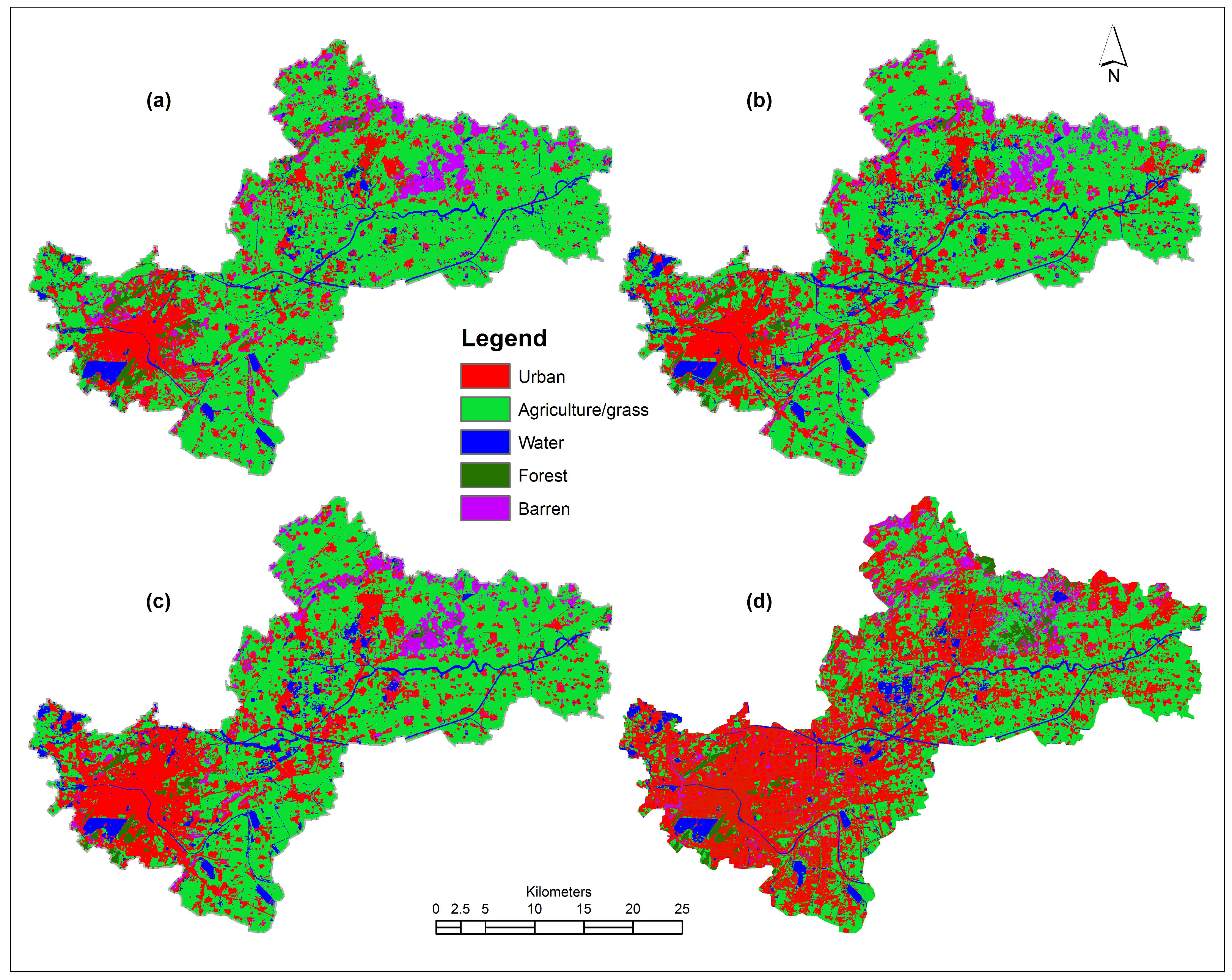
Two parameters should be defined in the RF classifier to generate a prediction model: the number of classification trees (k), and the number of prediction variables (m) used to split a RF node. In general, the generalization error always converges and over-training is not a problem due to the Strong Law of Large Numbers with increasing numbers of trees [53]. In order to decrease the strength of each individual tree of the model and reduce the correlation between trees, there is an effective approach to reduce the number of predictive variables (m). Thus, it is essential to optimize the parameters k and m to minimize the generalization error. In this study, based on the sensitivity experiment, we applied the RF classifier with 500 classification trees. The number of prediction variables (m) corresponds to the square root of the number of input variables [56]. Out-of-Bag (OOB) accuracy was employed to assess the performance of classification for each year, which is an unbiased estimator of the classification overall accuracy (OA) and can be used to substitute the cross-validation [51]. Approximately 2/3 of the train data were used to train the classifier, and the remaining data were used to validate the training. After classification, the mode filter (3 × 3) was used for post-classification procedures, like salt-and-pepper removal. Thus, the final LULC maps for 1985, 1995, 2005, and 2015 were generated (Figure 6).
2.4. Classification Accuracy Assessment
Accuracy assessment for individual classification is essential to correctly and efficiently analyze LULC change. The validation samples for each class using Google Earth and knowledge of the study area were collected based on the stratified random distribution method to conduct an accuracy assessment of each classification. The error matrix, overall accuracy, and Kappa coefficient were calculated for each classified land use map and tabulated in Table 1, Table 2, Table 3 and Table 4, respectively. The overall accuracies ranged from 95.56% to 98.46%, with Kappa coefficients from 0.9432 to 0.9803.
2.5. Land Use Change and Landscape Analysis
Land change analysis was carried out using geographic information system (GIS)-based spatial operations and landscape metrics derived from the LULC maps. In this paper, we focused on the land use changes during the periods of 1985–1995, 1995–2005, 2005–2015, and 1985–2015, especially on the growth of urban land and its spatial change trend. Several qualitative and quantitative methods were employed to analyze the spatial landscape patterns changes of land use at different stages. Here, landscape patterns were evaluated using landscape metrics, which can be calculated on the three different levels: patch, class, and landscape levels. In this study, class-level and landscape-level metrics were employed. Class-level metrics are used to qualify the characteristics of the same LULC type and return a unique value for each class in the landscape. Landscape-level metrics return a unique value corresponding to the landscape mosaic as a whole [57]. In order to reduce the correlativity, landscape metrics selected in this study are provided in Table 5 [58].
To visualize the spatiotemporal changes in landscape patterns and reveal their temporal and spatial characteristics during urbanization, the LULC maps of the four years were divided into 900 × 900 m grids using the gridsplitter plugin in Quantum GIS (QGIS, an official project of the Open Source Geospatial Foundation). A total of 1424 sub-grids were obtained in this study. The landscape metrics at the landscape level for each sub-grid were calculated using the Fragstats 4.2 (Oregon State University, Corvallis, OR, USA) to analyze the spatiotemporal changes in the landscape patterns.
3. Results and Analysis
3.1. Change Detection Analysis
The changes detections were implemented for 1985–1995, 1995–2005, 2005–2015, and 1985–2015. Firstly, we calculated the net area changes by category between the different years based on the LULC maps (Figure 7). Urban land has significantly increased, while the agricultural land was drastically reduced, which is supported in the Percentage of Landscape (PLAND) of different land uses in different years (Figure 8). During the period of 1985 to 1995, the urban area increased by 6082 ha, which is an increase of more than 30.65%. In the next two decades, the urban area increased by more than 10.54% and 68.78%, respectively (Figure 7, Figure 8 and Figure 9). This suggests a sharply ascending trend in the development of the urban area, especially from 2005 to 2015.
Figure 9 presents the gains and losses in urban area during the different periods. Agricultural land continually decreased, losing 26,933 ha in the 30-year period. Overall, the urban area significantly increased by about 143.75% in the study period, at the main expense of agricultural land in the area. Water bodies increased by 26.78%, which can be explained by the subsidence result from coal mining from 1985 to 1995. In the next two decades, the government attached importance to the reclamation of subsidence, so the water area slightly decreased by 5.72% and 15.90%, respectively. In general, there were no significant changes in the water body area. Forest increased by 15.68%, while barren land decreased by 28.63%. The transition mainly occurred from agricultural land to urban land from 1985 to 2015. Figure 10 illustrates the transition from other land use types to urban land in different periods.
3.2. Spatial Trend of Changes
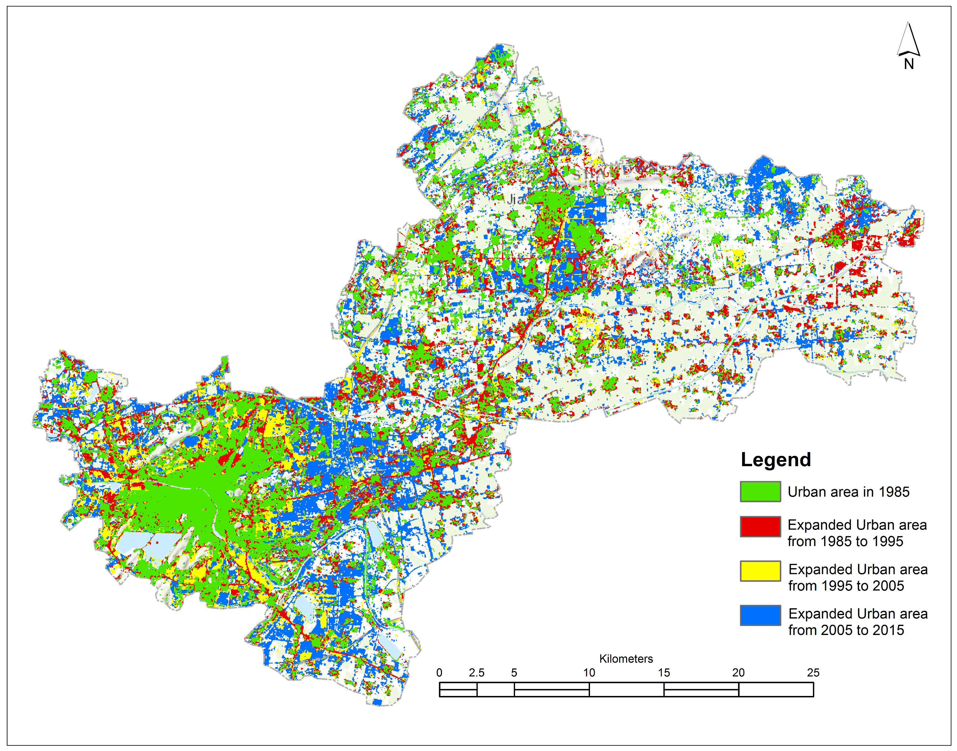
In landscapes dominated by human intervention, patterns of change can be complex, and thus difficult to decipher. Figure 11 shows the spatial sprawl of urban areas in 1985, 1995, 2005, and 2015. To reveal the spatial trend in urbanization, we created spatial trend maps of changes from other land types to urban land during the given periods adopting the ninth polynomial order (Figure 12).
As can be seen from the results, continuous transition occurred from other land use types into urban land via dual-core development throughout the urbanization process, which occurred in the main city region and Jiawang district, but with different development intensities in different periods. During 1985–1995, there was a continuous increase in the urban area between the two core regions from southwest to northeast (Figure 12a). In the subsequent 10 years, however, the expansion in the urban area mainly occurred in all directions around the two core regions, especially in the main city region (Figure 12b). During the period of 2005–2015, the growth in the southeastern part of the main city was mainly due to the construction of a new city region planned in 2004, which is also the location of the municipal government (Figure 12c). By the end of 2015, the total investment was around 70 billion yuan to construct the roads with a total length of about 110 km and 57 bridges, with a residential growth of more than 5 million m2 [59]. As can be seen in Figure 12c, the high railway station that became available in 2011 contributed to the growth in the urban area. Overall, in these three decades, the continuous increase in the urban area mainly occurred in the new city region and the Jiawang district, mainly affected by the construction of the new city region, a freeway, and the high railway station (Figure 12d). Compared with the digital elevation map (DEM) in Figure 12e, terrain was also one of the factors, affecting the spatial trend of urban area changes. In the southwest and northeast of the study area, the topography undulates considerably and the degree of urbanization was lower than in other areas.
3.3. Changes Analysis of Landscape Metrics
As shown in Figure 8 and Figure 10, the transition of land use types occurred mainly from agricultural land to urban land from 1985 to 2015. Thus, the changes and relationships measured based on different landscape metrics at the class level were analyzed between urban land and agricultural land (Figure 13). Here, the landscape metrics were fit into four major categories to represent different aspects of the landscape pattern: patch complexity (represented by PD, ED, and LSI), aggregation (represented by LPI and AI), connectivity (represented by COHESION), and diversity (represented by SHDI and SIDI) (Table 5).
3.4. Spatiotemporal Changes Analysis of Landscape Pattern
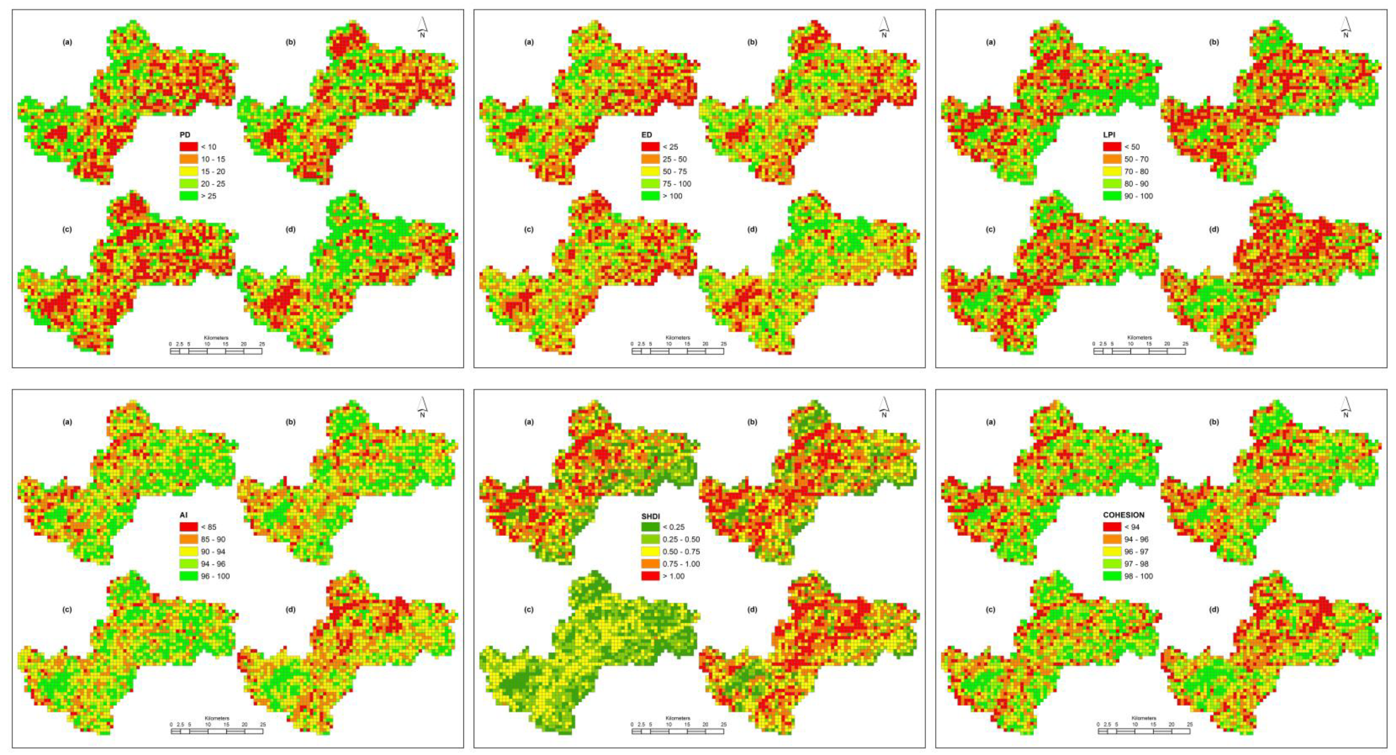
At the landscape level, landscape metrics calculated on the basis of sub-grids depict landscape pattern characteristics of each sub-grid and contribute to revealing the spatiotemporal changes in the study area. From the spatiotemporal changes in the landscape pattern, urban core, urban fringe, and rural area can be discerned. Here, we mapped the spatial distribution of each landscape metric for different years using the quantile grading method (Figure 15). The landscape patterns changed remarkably in the process of urbanization in Xuzhou.
For the PD landscape metric, urban core and rural areas were associated with lower values, mainly dominated by urban land and agricultural land, respectively, whereas urban fringe areas were the opposite. From the perspective of spatiotemporal changes, the urban core area expanded continuously, while the PD landscape metric in rural areas continued to increase, indicating that agricultural land continuously transitioned into urban land, demonstrating a tendency of fragmentation in the process of urbanization. AI, however, was opposite to PD, with higher values in the urban core and rural areas and lower values in urban fringes. As shown in Figure 15, ED and PD had a similar spatiotemporal change tendency. During urbanization, the values surrounding the urban core area slightly decreased, demonstrating that the core area continued to expand. From the southeast to the northeast of the main urban region, however, the value obviously increased, especially in 2015, mainly due to the construction of the new city region and the high railway station, resulting in considerable transformation of agricultural land into urban land. As LPI is used to quantify the percentage of the total landscape area of the largest patch, it is a simple measure of dominance. For instance, the LPI map Figure 15a depicts the prominence of the old city region and distribution of agricultural land. With the fragmentation of agricultural land, the LPI map (Figure 15d) clearly highlights the urban core area. The COHESION maps reveal the connectivity of the patches in the study area and represent the extent of the impact of urban expansion. Compared with the COHESION map in Figure 15a, the COHESION in Figure 15d obviously decreased in the southeast of the main city region, which verifies the vigorous development of the new city region. Regarding SHDI, although there was a marked decrease in 2005, SHDI significantly increased, mainly due to the continuous expansion of the urban area and the promotion of a large number of municipal projects, including the construction of freeways and subways. Considering the urban evolution, all landscape metrics used in this study were mutually corroborated in terms of spatiotemporal characteristics. The changes in landscape-level metrics in sub-grids effectively reveal the spatiotemporal evolution process of urbanization during the study period.
4. Discussion
4.1. NDEUI as an Effective Index for Improving the Classification Accuracy
The study of dramatic LULC change caused by urbanization is a major topic around the world. In China, the urbanization process has been accelerating. The study of LULC change caused by urbanization has attracted increasing attention, and a large amount of relevant research results have been published, especially for the extraction of urban areas based on indices [1,27,49]. A novel index, NDEUI, was proposed in this study, which combines annual maximum EVI and corresponding DMSP/OLS NTL, to effectively reduce confusion between urban areas and barren and fallow land. The advantage of this index is that annual maximum EVI ensures agricultural land has maximum EVI values, obtained during the growing season, to decrease the impact of seasonal fallow lands. Since barren land, especially far from urban area, is associated with extremely low NTL values, DMSP/OLS NTL can effectively separate them from urban lands. The 1-km resolution normalized NTL data must be downscaled to 30 m resolution. Firstly, we generated an annual maximum EVI from 32-day EVI composites for each year. Secondly, the NDEUI for each year was calculated. Afterward, a new composite was generated combining NTL, annual maximum EVI, and Landsat raw bands, which was used to obtain the land use classification using a random forests classifier. In this study, all the procedures were implemented on a free cloud computing platform, Google Earth Engine. GEE, based on its cloud computing and storage capability, has archived a large catalog of earth observation data that enables researchers to work on the trillions of online images. GEE represents one of the most powerful tools in remote sensing, given its ability to analyze and classify remotely sensed data over different temporal scales. In this study, GEE provided an effective approach to obtain the land cover classifications using JavaScript.
4.2. Relationship of Urbanization and Changes Dynamic of Landscape Pattern
The study of urban boundary extraction and sprawl analysis has attracted the attention of numerous researchers [12,60,61,62,63]. Analysis of the changes in landscape metrics has demonstrated the urban growth modes in the different processes of urbanization [12,35,64]. Some new landscape indices were proposed to quantitatively analyze changes in landscape patterns caused by urbanization [39,64]. Yang et al. [12] proposed a grid-based framework to analyze the influence of the landscape pattern on urban growth using multitemporal Landsat imagery. Usually, there are three urban growth modes discussed in the literature: Infilling, edge-expansion, and leapfrog mode [34,64,65]. In this study, several landscape metrics at the class and landscape level, depicted in detail in Section 3, were selected to characterize their spatiotemporal changes, generating a large quantity of information on landscape patterns. All of the information allowed us to determine which urban growth mode was dominant and the degrees of effects of urbanization at different stages during the study period. The gradual changes in landscape metrics imply that the landscape was undergoing a major transformation from one dominant land cover type to another due to urbanization. This dramatic land cover change caused by rapid urbanization has resulted in an essential change in landscape patterns. There are some inherent relationships between urbanization and the changes in landscape metrics, both at the class and landscape level. Consequently, studying urbanization using landscape metrics is essential.
Considering the urban growth modes, our analysis based on the results is as follows. With a slight increase in infilling area, urban growth mainly occurred in leapfrog mode along both sides of roads during the period from 1985 to 1995, resulting in a slightly decreased aggregation of the landscape. Subsequently, the urban growth mode shifted to edge-expansion. With increasing edge-expansion growth in urban areas, the urban land became increasingly aggregated and compact at this stage, especially in the main city region, reflected by the decreasing PD, ED, and LSI values and the increasing AI. Since 2005, the process of urbanization accelerated, and urban growth mainly appeared in the southeast to the northeast of the main city region due to the construction of a new city region and other infrastructure. During this stage, the edge-expansion and leapfrog modes coexisted, causing different degrees of change in the landscape metrics in different regions. The urbanization processes in different stages are reflected in the spatiotemporal changes of the landscape metrics.
5. Conclusions
Urbanization is an irreversible process, and rapid urbanization has resulted in drastic changes in LULC and landscape patterns since the 1980s, particularly in developing countries. Mapping and monitoring of LULC change, therefore, is crucial to generating information for policymakers and planners, as well as for understanding the underlying socio-economic and biophysical processes in urban areas. Accordingly, a GIS- and RS-based integrated approach was used to quantitatively characterize the LULC pattern and dynamics of urban sprawl in Xuzhou, China during the period of 1985 to 2015.
In this study, we integrated NTL with annual maximum EVI and proposed a new spectral index, NDEUI. An NDEUI-assisted Random Forests algorithm was implemented to obtain the LULC maps in 1985, 1995, 2005, and 2015. The results indicate that the proposed classification scheme was more accurate, reducing confusion between urban areas and barren land. The results show that Xuzhou has experienced rapid urbanization since the 1980s. Urban areas increased by 143.75%, approximately 2.44 times greater than the urban area in 1985, resulting in a considerable decrease in agricultural land. Among the three decades, the highest growth in urban land was 68.78% from 2005 to 2015, averaging nearly 7% per year. As can be seen from the analysis of the urban growth spatial trend that urban growth proceeded in different directions during the different periods. Overall, the urban growth occurred in dual-core development mode throughout the urbanization process. The process of urbanization in the northeast area of the main city region occurred due to a growth in the industrial area in the first two decades, whereas, in the southeastern direction, the urban growth was mostly due to the construction of a new city region that was planned in 2004 and the high railway station that became available in 2011, accompanied by growth of residential areas. Notably, terrain and roads were also important factors affecting urbanization.
Statistical analysis may have limited power to demonstrate the inherent relationship between LULC changes; accordingly, the dynamic changes of landscape pattern affected by urbanization were studied. Six landscape metrics at the class level were calculated to reveal the dynamic changes in landscape patterns in urban and agricultural land. The changes in the selected landscape metrics indicate a lower aggregation and connectivity in agricultural land due to increasing dominance of urban land during the study period. Nine landscape metrics were also calculated to indicate the landscape metrics changes at the landscape level. The landscape-level metrics changes suggest an increasing spatial heterogeneity along with the process of rapid urbanization during 1985–2015. To visualize the spatiotemporal changes in landscape patterns and reveal their temporal and spatial characteristics during urbanization, we divided all the LULC maps into 900 × 900 m sub-grids and calculated their landscape metrics at the landscape level. The findings suggest that different urbanization modes and intensities result in various spatiotemporal evolutions of landscape patterns. In terms of the urban growth mode, the urban growth mainly occurred in leapfrog mode along both sides of the roads during the period of 1985 to 1995, and then shifted into edge-expansion mode during the period of 1995 to 2005, whereas the edge-expansion and leapfrog modes coexisted during the period of 2005 to 2015, causing different degrees of change in the landscape metrics in different regions. Overall, the highly valuable spatiotemporal information generated using RS and GIS may assist urban planners and policymakers to better understand urban dynamics and evaluate their spatiotemporal and environmental impacts at the local level to enable sustainable urban planning in the future.
Author Contributions
Data curation, Y.X. and C.L.; Supervision, N.X.T.; Writing—original draft, Y.X.
Funding
Visiting Research Scholar Program of the China Scholarship Council (Grant No. 201606425072), Priority Academic Program Development of Jiangsu Higher Education Institutions (PAPD).
Acknowledgments
We would like to express our respect and gratitude to the anonymous reviewers and editors for their professional comments and suggestions on improving the quality of this paper. This work was supported by the Visiting Research Scholar Program of the China Scholarship Council (Grant No. 201606425072), A Project Funded by the Priority Academic Program Development of Jiangsu Higher Education Institutions (PAPD).
Conflicts of Interest
The authors declare no conflict of interest.
References
- Zhang, J.; Li, P.J.; Wang, J.F. Urban Built-up Area Extraction from Landsat TM/ETM plus Images Using Spectral Information and Multivariate Texture. Remote Sens. 2014, 6, 7339–7359. [Google Scholar] [CrossRef]
- Reynolds, R.; Liang, L.; Li, X.C.; Dennis, J. Monitoring Annual Urban Changes in a Rapidly Growing Portion of Northwest Arkansas with a 20-Year Landsat Record. Remote Sens. 2017, 9, 71. [Google Scholar] [CrossRef]
- Verhasselt, Y. Urbanization and Health in the Developing World. Soc. Sci. Med. 1985, 21, 483. [Google Scholar] [CrossRef]
- Minshull, R. Urbanisation: Changing environments. Geography 1998, 83, 297. [Google Scholar]
- Li, X.; Gong, P.; Liang, L. A 30-year (1984–2013) record of annual urban dynamics of Beijing City derived from Landsat data. Remote Sens. Environ. 2015, 166, 78–90. [Google Scholar] [CrossRef]
- Li, X.C.; Liu, X.P.; Gong, P. Integrating ensemble-urban cellular automata model with an uncertainty map to improve the performance of a single model. Int. J. Geogr. Inf. Sci. 2015, 29, 762–785. [Google Scholar] [CrossRef]
- Zhang, P.; Imhoff, M.L.; Bounoua, L.; Wolfe, R.E. Exploring the influence of impervious surface density and shape on urban heat islands in the northeast United States using MODIS and Landsat. Can. J. Remote Sens. 2012, 38, 441–451. [Google Scholar]
- Ceplova, N.; Kalusova, V.; Lososova, Z. Effects of settlement size, urban heat island and habitat type on urban plant biodiversity. Landsc. Urban Plan. 2017, 159, 15–22. [Google Scholar] [CrossRef]
- Schneider, A. Monitoring land cover change in urban and pen-urban areas using dense time stacks of Landsat satellite data and a data mining approach. Remote Sens. Environ. 2012, 124, 689–704. [Google Scholar] [CrossRef]
- Lu, M.; Chen, J.; Tang, H.J.; Rao, Y.H.; Yang, P.; Wu, W.B. Land cover change detection by integrating object-based data blending model of Landsat and MODIS. Remote Sens. Environ. 2016, 184, 374–386. [Google Scholar] [CrossRef]
- Coulter, L.L.; Stow, D.A.; Tsai, Y.H.; Ibanez, N.; Shih, H.C.; Kerr, A.; Benza, M.; Weeks, J.R.; Mensah, F. Classification and assessment of land cover and land use change in southern Ghana using dense stacks of Landsat 7 ETM + imagery. Remote Sens. Environ. 2016, 184, 396–409. [Google Scholar] [CrossRef]
- Yang, Y.T.; Wong, L.N.Y.; Chen, C.; Chen, T. Using multitemporal Landsat imagery to monitor and model the influences of landscape pattern on urban expansion in a metropolitan region. J. Appl. Remote Sens. 2014, 8, 083639. [Google Scholar] [CrossRef]
- Mihai, B.; Nistor, C.; Simion, G. Post-socialist urban growth of Bucharest, Romania—A change detection analysis on Landsat imagery (1984–2010). Acta Geogr. Slov. 2015, 55, 223–234. [Google Scholar] [CrossRef]
- Schneider, A.; Friedl, M.A.; Potere, D. A new map of global urban extent from MODIS satellite data. Environ. Res. Lett. 2009, 4, 044003. [Google Scholar] [CrossRef] [Green Version]
- Xian, G.; Homer, C.; Demitz, J.; Fry, J.; Hossain, N.; Wickham, J. Change of Impervious Surface Area Between 2001 and 2006 in the Conterminous United States. Photogramm. Eng. Remote Sens. 2011, 77, 758–762. [Google Scholar]
- Gong, P.; Wang, J.; Yu, L.; Zhao, Y.C.; Zhao, Y.Y.; Liang, L.; Niu, Z.G.; Huang, X.M.; Fu, H.H.; Liu, S.; et al. Finer resolution observation and monitoring of global land cover: First mapping results with Landsat TM and ETM+ data. Int. J. Remote Sens. 2013, 34, 2607–2654. [Google Scholar] [CrossRef]
- Selkowitz, D.J.; Stehman, S.V. Thematic accuracy of the National Land Cover Database (NLCD) 2001 land cover for Alaska. Remote Sens. Environ. 2011, 115, 1401–1407. [Google Scholar]
- Han, R.; Li, Z.L.; Ti, P.; Xu, Z. Experimental Evaluation of the Usability of Cartogram for Representation of GlobeLand30 Data. ISPRS Int. J. Geo-Inf. 2017, 6, 180. [Google Scholar] [CrossRef]
- Liang, D.; Zuo, Y.; Huang, L.S.; Zhao, J.L.; Teng, L.; Yang, F. Evaluation of the Consistency of MODIS Land Cover Product (MCD12Q1) Based on Chinese 30 m GlobeLand30 Datasets: A Case Study in Anhui Province, China. ISPRS Int. J. Geo-Inf. 2015, 4, 2519–2541. [Google Scholar] [CrossRef] [Green Version]
- Li, G.; Lu, D.; Moran, E.; Hetrick, S. Mapping impervious surface area in the Brazilian Amazon using Landsat Imagery. Gisci. Remote Sens. 2013, 50, 172–183. [Google Scholar] [CrossRef] [PubMed]
- Lu, D.S.; Weng, Q.H. Spectral mixture analysis of the urban landscape in Indianapolis with landsat ETM plus imagery. PPhotogramm. Eng. Remote Sens. 2004, 70, 1053–1062. [Google Scholar] [CrossRef]
- Boldt, M.; Thiele, A.; Schulz, K. Object-based Urban Change Detection Analyzing High Resolution Optical Satellite Images. Int. Soc. Opt. Eng. 2012. [Google Scholar] [CrossRef]
- Darwish, A.; Leukert, K.; Reinhardt, W. Urban land-cover classification: An object based perspective. In Proceedings of the 2nd Grss/ISPRS Joint Workshop on Remote Sensing and Data Fusion over Urban Areas, Berlin, Germany, 22–23 May 2003; pp. 278–282. [Google Scholar]
- Zhang, Q.L.; Li, B.; Thau, D.; Moore, R. Building a Better Urban Picture: Combining Day and Night Remote Sensing Imagery. Remote Sens. 2015, 7, 11887–11913. [Google Scholar] [CrossRef] [Green Version]
- Liu, C.; Shao, Z.F.; Chen, M.; Luo, H. MNDISI: A multi-source composition index for impervious surface area estimation at the individual city scale. Remote Sens. Lett. 2013, 4, 803–812. [Google Scholar] [CrossRef]
- Deng, C.B.; Wu, C.S. BCI: A biophysical composition index for remote sensing of urban environments. Remote Sens. Environ. 2012, 127, 247–259. [Google Scholar] [CrossRef]
- As-Syakur, A.R.; Adnyana, I.W.S.; Arthana, I.W.; Nuarsa, I.W. Enhanced Built-Up and Bareness Index (EBBI) for Mapping Built-Up and Bare Land in an Urban Area. Remote Sens. 2012, 4, 2957–2970. [Google Scholar] [CrossRef] [Green Version]
- Li, S.; Chen, X. A new bare-soil index for rapid mapping developing areas using LANDSAT 8 data. ISPRS Int. Arch. Photogramm. Remote Sens. Spat. Inf. Sci. 2014, XL-4, 139–144. [Google Scholar] [CrossRef]
- Lu, D.; Mausel, P.; Brondizio, E.; Moran, E. Change detection techniques. Int. J. Remote Sens. 2004, 25, 2365–2407. [Google Scholar] [CrossRef]
- Tewkesbury, A.P.; Comber, A.J.; Tate, N.J.; Lamb, A.; Fisher, P.F. A critical synthesis of remotely sensed optical image change detection techniques. Remote Sens. Environ. 2015, 160, 1–14. [Google Scholar] [CrossRef] [Green Version]
- Jackson, T.J.; Chen, J.M.; Gong, P.; Liang, S.; Hassan, M.A. Integration of remote sensing (RS) and geographic information system (GIS) techniques for change detection of the land use and land cover (LULC) for soil management in the southern Port Said region, Egypt. Land Surf. Remote Sens. 2014, 9260, 926032. [Google Scholar]
- Son, N.T.; Chen, C.F.; Chen, C.R.; Chang, L.Y.; Thanh, B.X. Urban growth mapping from Landsat data using linear mixture model in Ho Chi Minh City, Vietnam. J. Appl. Remote Sens. 2012, 6, 063543. [Google Scholar]
- Villa, P. Mapping urban growth using Soil and Vegetation Index and Landsat data: The Milan (Italy) city area case study. Landsc. Urban Plan. 2012, 107, 245–254. [Google Scholar] [CrossRef]
- Li, H.; Peng, J.; Yanxu, L.; Yi’na, H. Urbanization impact on landscape patterns in Beijing City, China: A spatial heterogeneity perspective. Ecol. Indic. 2017, 82, 50–60. [Google Scholar] [CrossRef]
- Chan, K.M.; Vu, T.T. A landscape ecological perspective of the impacts of urbanization on urban green spaces in the Klang Valley. Appl. Geogr. 2017, 85, 89–100. [Google Scholar] [CrossRef]
- Krajewski, P. Assessing Change in a High-Value Landscape: Case Study of the Municipality of Sobotka, Poland. Pol. J. Environ. Stud. 2017, 26, 2603–2610. [Google Scholar] [CrossRef] [Green Version]
- Schwoertzig, E.; Poulin, N.; Hardion, L.; Trémolières, M. Plant ecological traits highlight the effects of landscape on riparian plant communities along an urban-rural gradient. Ecol. Indic. 2016, 61, 568–576. [Google Scholar] [CrossRef]
- Liu, T.; Yang, X.J. Monitoring land changes in an urban area using satellite imagery, GIS and landscape metrics. Appl. Geogr. 2015, 56, 42–54. [Google Scholar] [CrossRef]
- Krajewski, P.; Solecka, I. Barbara-Mastalska-Cetera, Landscape Change Index as a Tool for Spatial Analysis. In Proceedings of the World Multidisciplinary Civil Engineering-Architecture-Urban Planning Symposium—Wmcaus, Prague, Czech, 12–16 June 2017; p. 245. [Google Scholar]
- Chander, G.; Markham, B.L.; Helder, D.L. Summary of current radiometric calibration coefficients for Landsat MSS, TM, ETM+, and EO-1 ALI sensors. Remote Sens. Environ. 2009, 113, 893–903. [Google Scholar] [CrossRef] [Green Version]
- Huete, A.; Didan, K.; Miura, T.; Rodriguez, E.P.; Gao, X.; Ferreira, L.G. Overview of the radiometric and biophysical performance of the MODIS vegetation indices. Remote Sens. Environ. 2002, 83, 195–213. [Google Scholar] [CrossRef]
- Earth Observation Group. Defense Meteorological Satellite Progam, Boulder | ngdc.noaa.gov. Available online: https://ngdc.noaa.gov/eog/dmsp/downloadV4composites.html (accessed on 10 July 2017).
- Tan, M.H. Urban Growth and Rural Transition in China Based on DMSP/OLS Nighttime Light Data. Sustainability 2015, 7, 8768–8781. [Google Scholar] [CrossRef] [Green Version]
- Liu, Z.F.; He, C.Y.; Zhang, Q.F.; Huang, Q.X.; Yang, Y. Extracting the dynamics of urban expansion in China using DMSP-OLS nighttime light data from 1992 to 2008. Landsc. Urban Plan. 2012, 106, 62–72. [Google Scholar] [CrossRef]
- Elvidge, C.; Hsu, F.-C.; Baugh, K.; Ghosh, T. National Trends in Satellite-Observed Lighting: 1992–2012. In Global Urban Monitoring and Assessment through Earth Observation; CRC Press: Boca Raton, FL, USA, 2013; pp. 97–120. [Google Scholar]
- Pandey, B.; Zhang, Q.L.; Seto, K.C. Comparative evaluation of relative calibration methods for DMSP/OLS nighttime lights. Remote Sens. Environ. 2017, 195, 67–78. [Google Scholar] [CrossRef]
- Zhang, Q.L.; Pandey, B.; Seto, K.C. A Robust Method to Generate a Consistent Time Series from DMSP/OLS Nighttime Light Data. IEEE Trans. Geosci. Remote Sens. 2016, 54, 5821–5831. [Google Scholar] [CrossRef]
- Zhang, Q.L.; Schaaf, C.; Seto, K.C. The Vegetation Adjusted NTL Urban Index: A new approach to reduce saturation and increase variation in nighttime luminosity. Remote Sens. Environ. 2013, 129, 32–41. [Google Scholar] [CrossRef]
- Cheng, Y.; Zhao, L.M.; Wan, W.; Li, L.L.; Yu, T.; Gu, X.F. Extracting urban areas in China using DMSP/OLS nighttime light data integrated with biophysical composition information. J. Geogr. Sci. 2016, 26, 325–338. [Google Scholar] [CrossRef]
- Schneider, A.; Mertes, C.M. Expansion and growth in Chinese cities, 1978–2010. Environ. Res. Lett. 2014, 9, 024008. [Google Scholar] [CrossRef] [Green Version]
- Breiman, L. Random forests. Mach. Learn. 2001, 45, 5–32. [Google Scholar] [CrossRef]
- Rodriguez-Galiano, V.F.; Ghimire, B.; Rogan, J.; Chica-Olmo, M.; Rigol-Sanchez, J.P. An assessment of the effectiveness of a random forest classifier for land-cover classification. ISPRS J. Photogramm. Remote Sens. 2012, 67, 93–104. [Google Scholar] [CrossRef]
- Breiman, L. Bagging predictors. Mach. Learn. 1996, 24, 123–140. [Google Scholar] [CrossRef] [Green Version]
- Gislason, P.O.; Benediktsson, J.A.; Sveinsson, J.R. Random Forests for land cover classification. Pattern Recogn. Lett. 2006, 27, 294–300. [Google Scholar] [CrossRef]
- Chan, J.C.-W.; Paelinckx, D. Evaluation of Random Forest and Adaboost tree-based ensemble classification and spectral band selection for ecotope mapping using airborne hyperspectral imagery. Remote Sens. Environ. 2008, 112, 2999–3011. [Google Scholar] [CrossRef]
- Pelletier, C.; Valero, S.; Inglada, J.; Champion, N.; Dedieu, G. Assessing the robustness of Random Forests to map land cover with high resolution satellite image time series over large areas. Remote Sens. Environ. 2016, 187, 156–168. [Google Scholar] [CrossRef]
- Cushman, S.A.; McGariyal, K.; Neel, M.C. Parsimony in landscape metrics: Strength, universality, and consistency. Ecol. Indic. 2008, 8, 691–703. [Google Scholar] [CrossRef]
- McGarigal, K.; Cushman, S.; Ene, E. FRAGSTATS v4: Spatial Pattern Analysis Program for Categorical and Continuous Maps. Computer Software Program Produced by the Authors at the University of Massachusetts, Amherst. Available online: http://www.umass.edu/landeco/research/fragstats/fragstats.html (accessed on 23 January 2015).
- Report on the Work of Xuzhou Municipal Government in 2016; Xuzhou Municipal Government: Xuzhou, China, 2016. Available online: http://district.ce.cn/newarea/roll/201602/25/t20160225_9097273.shtml (accessed on 10 September 2017).
- Peng, J.; Zhao, M.Y.; Guo, X.N.; Pan, Y.J.; Liu, Y.X. Spatial-temporal dynamics and associated driving forces of urban ecological land: A case study in Shenzhen City, China. Habitat Int. 2017, 60, 81–90. [Google Scholar] [CrossRef]
- Dou, P.; Chen, Y.B. Dynamic monitoring of land-use/land-cover change and urban expansion in Shenzhen using Landsat imagery from 1988 to 2015. Int. J. Remote Sens. 2017, 38, 5388–5407. [Google Scholar] [CrossRef]
- Chen, Y.J.; Yu, S.X. Assessment of urban growth in Guangzhou using multi-temporal, multi-sensor Landsat data to quantify and map impervious surfaces. Int. J. Remote Sens. 2016, 37, 5936–5952. [Google Scholar] [CrossRef]
- Hu, S.G.; Tong, L.Y.; Frazier, A.E.; Liu, Y.S. Urban boundary extraction and sprawl analysis using Landsat images: A case study in Wuhan, China. Habitat Int. 2015, 47, 183–195. [Google Scholar] [CrossRef] [Green Version]
- Liu, X.P.; Li, X.; Chen, Y.M.; Tan, Z.Z.; Li, S.Y.; Ai, B. A new landscape index for quantifying urban expansion using multi-temporal remotely sensed data. Landsc. Ecol 2010, 25, 671–682. [Google Scholar] [CrossRef]
- Sun, C.; Wu, Z.F.; Lv, Z.Q.; Yao, N.; Wei, J.B. Quantifying different types of urban growth and the change dynamic in Guangzhou using multi-temporal remote sensing data. Int. J. Appl. Earth Obs. Geoinf. 2013, 21, 409–417. [Google Scholar] [CrossRef] [Green Version]
Figure 1.
(a) Map of China showing the location of Jiangsu province (Data Source: ESRI); (b) Map of Jiangsu province showing the location of Xuzhou city center (Data Source: ESRI); and (c) map of study area.
Figure 1.
(a) Map of China showing the location of Jiangsu province (Data Source: ESRI); (b) Map of Jiangsu province showing the location of Xuzhou city center (Data Source: ESRI); and (c) map of study area.

Figure 2.
Population, built-up area and gross domestic product (GDP) growth of Xuzhou from 1978 to 2014 (Data Source: Statistical Yearbook of Xuzhou City). Note: In 1993 and 2000, some administrative divisions were adjusted.
Figure 2.
Population, built-up area and gross domestic product (GDP) growth of Xuzhou from 1978 to 2014 (Data Source: Statistical Yearbook of Xuzhou City). Note: In 1993 and 2000, some administrative divisions were adjusted.

Figure 3.
Flowchart of the procedural workflow.

Figure 4.
Multispectral seasonal observations of built-up land and cropland from 30-m resolution Landsat TM data in 2005 (a–e) in a peri-urban area northwest of Xuzhou (the Near-infrared, Red, and Green wavelengths were set to R-G-B, respectively. A reference of the same area is shown in (e) from Google Earth).
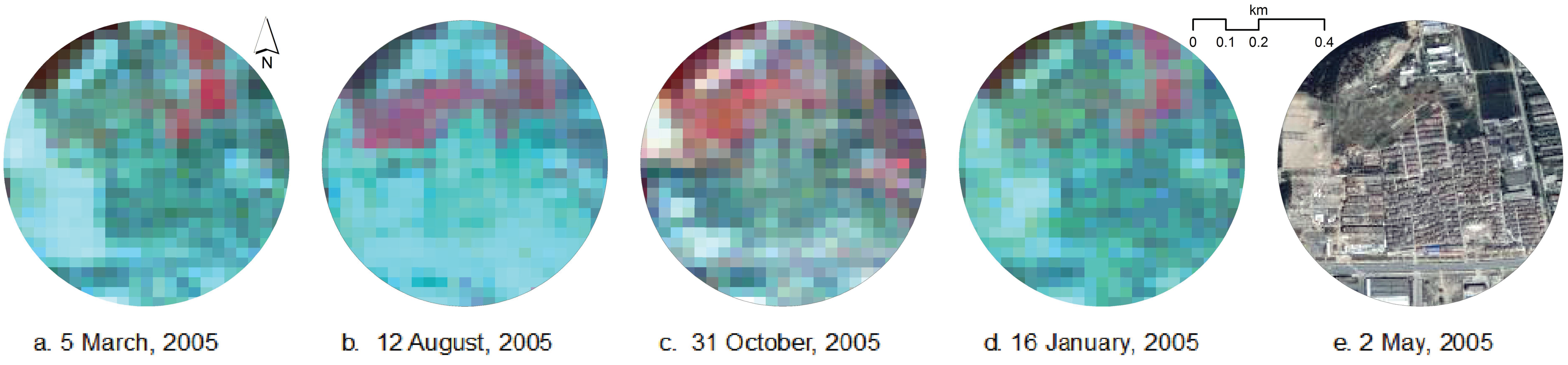
Figure 5.
Comparison between the NDVI and EVI, derived from the Landsat 8 32-day NDVI composite and EVI composite in 2016.
Figure 5.
Comparison between the NDVI and EVI, derived from the Landsat 8 32-day NDVI composite and EVI composite in 2016.

Figure 6.
Land use and land cover (LULC) maps of Xuzhou city for (a) 1985, (b) 1995, (c) 2005, and (d) 2015 derived from Landsat series imageries.
Figure 6.
Land use and land cover (LULC) maps of Xuzhou city for (a) 1985, (b) 1995, (c) 2005, and (d) 2015 derived from Landsat series imageries.

Figure 7.
Net area changes by category between different years.

Figure 8.
The proportion of area for each class type in the landscape.

Figure 9.
Maps presenting gains and losses in urban area during the period of (a) 1985–1995, (b) 1995–2005, (c) 2005–2015, and (d) 1985–2015.
Figure 9.
Maps presenting gains and losses in urban area during the period of (a) 1985–1995, (b) 1995–2005, (c) 2005–2015, and (d) 1985–2015.
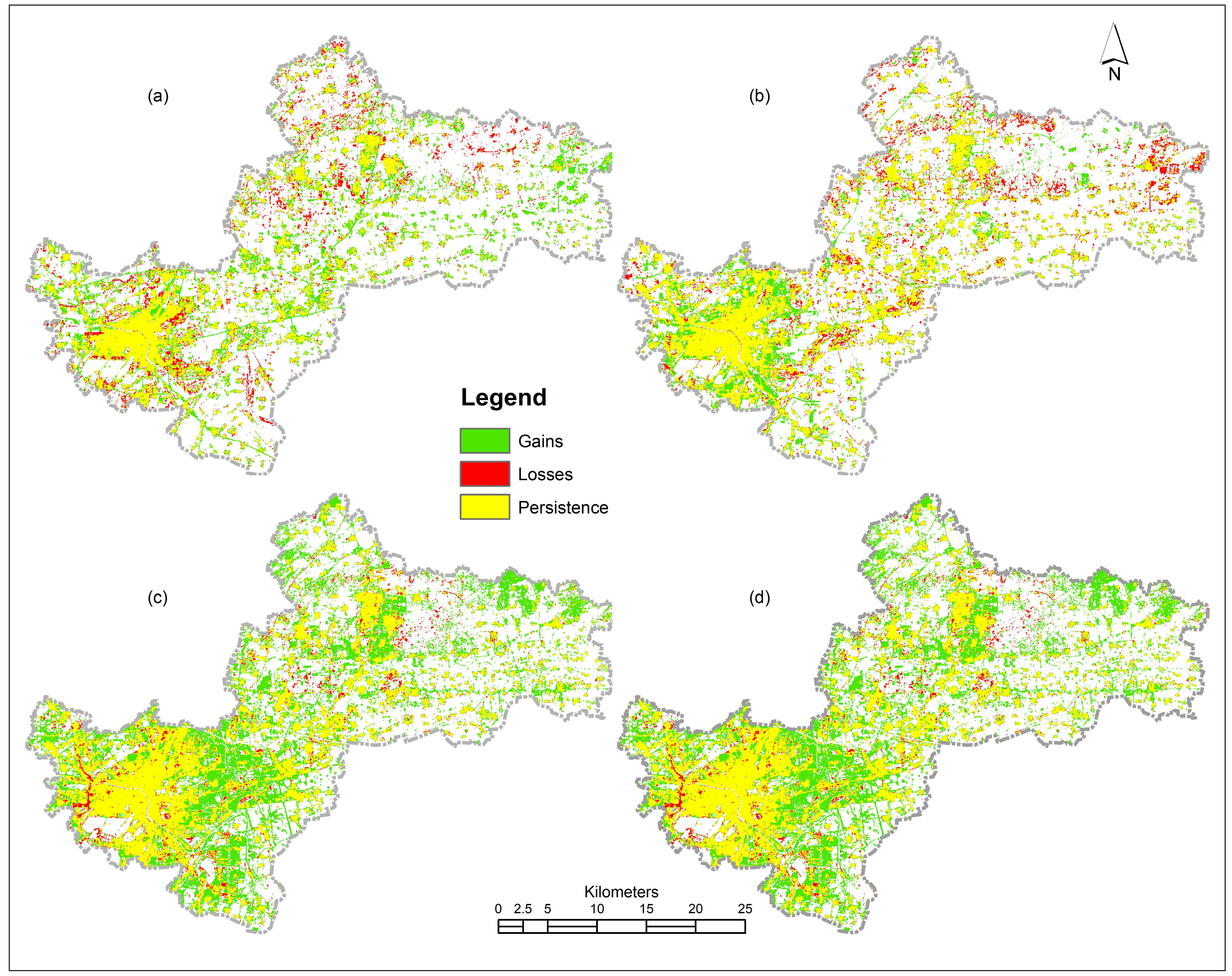
Figure 10.
Maps of land use transition from other land use types to urban land during (a) 1985–1995, (b) 1995–2005, (c) 2005–2015, and (d) 1985–2015.
Figure 10.
Maps of land use transition from other land use types to urban land during (a) 1985–1995, (b) 1995–2005, (c) 2005–2015, and (d) 1985–2015.
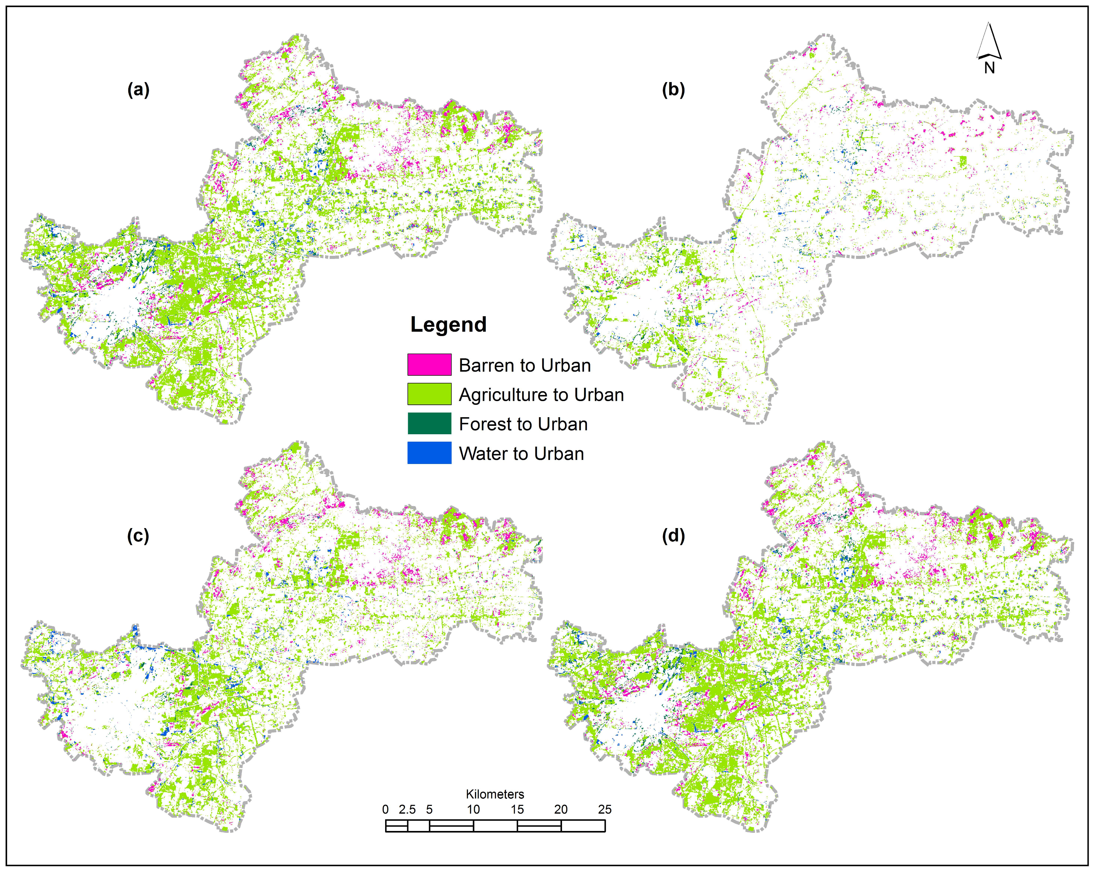
Figure 11.
Spatial forms of urban sprawl in 1985, 1995, 2005, and 2015.

Figure 12.
Spatial trend in urban growth during (a) 1985–1995, (b) 1995–2005, (c) 2005–2015, and (d) 1985–2015, and (e) digital elevation map (DEM) of the study area.
Figure 12.
Spatial trend in urban growth during (a) 1985–1995, (b) 1995–2005, (c) 2005–2015, and (d) 1985–2015, and (e) digital elevation map (DEM) of the study area.

Figure 13.
All landscape metrics of urban and agricultural land underwent tremendous changes during the study period. In terms of PD, urban land use trended downward while agricultural land use continuously increased. (a) In terms of PD, urban land use trended downward while agricultural land use continuously increased. (b) On the contrary, there was a consistent trend in the changes in the ED of agricultural land and urban land, reaching the lowest values in 2005, then dramatically increasing up to 48.853m/ha and 55.9287 m/ha in 2015, respectively. (c) Considering urban land, the dates for LSI are interesting: the values decreased rapidly from 75.4532 in 1985 to 58.1453 in 2005, but then increased again to 68.1731 in 2015. The LSI of agricultural land increased overall increase from 41.6725 in 1985 to 64.2222 in 2015, except for a slight decrease in 2005. (d) Illustrates that with a significant decrease in the LPI of agricultural land, the LPI of urban land continued to increase, with an increase of more than 18.5%. Meanwhile, there was a gradual increase in the AI of urban land, reaching 90.8229% in 2015. In terms of agricultural land, however, the AI gradually dropped from 95.3672% in 1985 to 90.7922% in 2015. (e) Meanwhile, there was a gradual increase in the AI of urban land, reaching 90.8229% in 2015. In terms of agricultural land, however, the AI gradually dropped from 95.3672% in 1985 to 90.7922% in 2015. (f) The aggregation of urban land gradually increased and surpassed that of agricultural land during the 30-year process of urbanization. With regards to COHESION, the values of agricultural land changed from 99.8371 to 99.0596, and urban land from 97.7713 to 99.6485 during the study period.

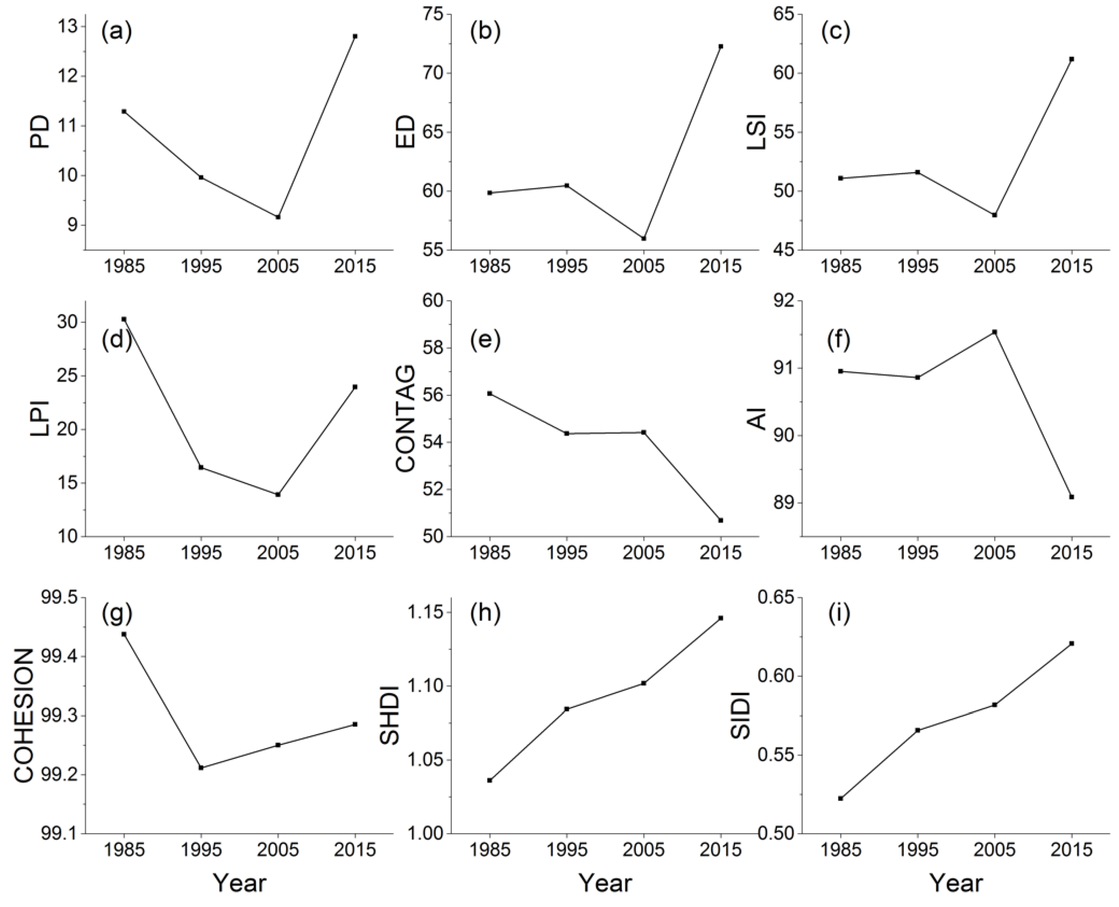
Figure 14.
Line graphs depicting the landscape-level metrics changes from 1985 to 2015. (a) PD, (b) ED, (c) LSI, (d) LPI, (e) CONTAG, (f) AI, (g) COHESION, (h) SHDI, (i) SIDI. (a–c) There were the lowest patch complexity in 2005, increasing to a maximum in 2015. The highest rates of change in the three metrics were observed in the period between 2005 and 2015. In terms of urbanization modes, this may indicate that infilling and edge-expansion modes were dominant in Xuzhou before 2005, and then leapfrog mode dominated. (d) LPI declined from 30.2737% in 1985 to 13.9131% in 2005, which may provide evidence that agricultural land was dominant in 1985. However, LPI increased again to 23.9468% in 2015. (e,f) The CONTAG and AI metrics were inversely related to LSI. They slightly fluctuated, but then dramatically decreased after 2005. This tendency confirms that the landscape pattern was vastly disaggregated and less contiguous in 2015, mainly owing to continued increasing leapfrog urban land. (g) Shows the changes in COHESION. The COHESION value decreased sharply, reaching its lowest value of 99.2116 in 1995. Thereafter, it increased continuously in the later stages of urbanization. (h,i) Both SHDI and SIDI measure relative diversity. From 1985 to 2015, the two diversity metrics increased constantly, indicating an increasing heterogeneity of this landscape. This fact is evident as agriculture segmented into smaller patches with the continual increase in urban land.

Figure 15.
Spatiotemporal changes of landscape metrics: (a) 1985, (b) 1995, (c) 2005, and (d) 2015.


Table 1.
Accuracy assessment for the 1985 land use and land cover (LULC) map produced from Landsat TM.
Table 1.
Accuracy assessment for the 1985 land use and land cover (LULC) map produced from Landsat TM.
| Classified Data | Reference Data | User’s Accuracy (%) | Kappa Accuracy | |||||
|---|---|---|---|---|---|---|---|---|
| C1 | C2 | C3 | C4 | C5 | Sum | |||
| Urban land (C1) | 181 | 1 | 3 | 9 | 194 | 93.30 | 0.9124 | |
| Agriculture/grass land (C2) | 256 | 256 | 100 | 1 | ||||
| Water bodies (C3) | 1 | 141 | 3 | 145 | 97.24 | 0.9670 | ||
| Forest (C4) | 1 | 114 | 115 | 99.13 | 0.9899 | |||
| Barren land (C5) | 20 | 125 | 145 | 86.21 | 0.8364 | |||
| Sum | 201 | 259 | 141 | 120 | 134 | 885 | ||
| Producer’s Accuracy (%) | 90.05 | 98.84 | 100 | 95.00 | 93.28 | |||
| Overall Accuracy (%) | 95.56 | |||||||
| Kappa Coefficient | 0.9432 | |||||||
Table 2.
Accuracy assessment for the 1995 LULC map produced from Landsat TM.
| Classified Data | Reference Data | User’s Accuracy (%) | Kappa Accuracy | |||||
|---|---|---|---|---|---|---|---|---|
| C1 | C2 | C3 | C4 | C5 | Sum | |||
| Urban land (C1) | 241 | 2 | 243 | 99.18 | 0.9892 | |||
| Agriculture/grass land (C2) | 293 | 293 | 100 | 1 | ||||
| Water bodies (C3) | 2 | 203 | 6 | 211 | 96.21 | 0.9529 | ||
| Forest (C4) | 145 | 145 | 100 | 1 | ||||
| Barren land (C5) | 8 | 144 | 152 | 94.74 | 0.9388 | |||
| Sum | 249 | 295 | 203 | 151 | 146 | 1044 | ||
| Producer’s Accuracy (%) | 96.79 | 99.32 | 100 | 96.03 | 98.63 | |||
| Overall Accuracy (%) | 98.28 | |||||||
| Kappa Coefficient | 0.9780 | |||||||
Table 3.
Accuracy assessment for the 2005 LULC map produced from Landsat TM.
| Classified Data | Reference Data | User’s Accuracy (%) | Kappa Accuracy | |||||
|---|---|---|---|---|---|---|---|---|
| C1 | C2 | C3 | C4 | C5 | Sum | |||
| Urban land (C1) | 300 | 1 | 3 | 304 | 98.68 | 0.9825 | ||
| Agriculture/grass land (C2) | 353 | 1 | 354 | 99.72 | 99.60 | |||
| Water bodies (C3) | 209 | 3 | 212 | 98.58 | 98.30 | |||
| Forest (C4) | 193 | 193 | 100 | 1 | ||||
| Barren land (C5) | 8 | 1 | 2 | 157 | 168 | 93.45 | 0.9247 | |
| Sum | 308 | 355 | 209 | 199 | 160 | 1231 | ||
| Producer’s Accuracy (%) | 97.40 | 99.44 | 100 | 96.98 | 98.18 | |||
| Overall Accuracy (%) | 98.46 | |||||||
| Kappa Coefficient | 0.9803 | |||||||
Table 4.
Accuracy assessment for the 2015 LULC map produced from Landsat OLI.
| Classified Data | Reference Data | User’s Accuracy (%) | Kappa Accuracy | |||||
|---|---|---|---|---|---|---|---|---|
| C1 | C2 | C3 | C4 | C5 | Sum | |||
| Urban land (C1) | 338 | 3 | 8 | 349 | 96.85 | 0.9182 | ||
| Agriculture/grass land (C2) | 1 | 350 | 3 | 354 | 98.87 | 0.9755 | ||
| Water bodies (C3) | 1 | 1 | 253 | 255 | 99.22 | 1 | ||
| Forest (C4) | 199 | 199 | 100 | 1 | ||||
| Barren land (C5) | 21 | 1 | 123 | 145 | 84.83 | 1 | ||
| Sum | 361 | 351 | 253 | 203 | 134 | 1302 | ||
| Producer’s Accuracy (%) | 93.63 | 99.72 | 100 | 98.03 | 91.79 | |||
| Overall Accuracy (%) | 97.00 | |||||||
| Kappa Coefficient | 0.9615 | |||||||
Table 5.
List and descriptions of landscape metrics used in this study.
| Landscape Metrics | Description | Level | Unit | Range |
|---|---|---|---|---|
| General index | ||||
| PLAND (Percentage landscape) | To quantify the proportional abundance of each patch type in the landscape | Class | Percent | 0 < PLAND ≤ 100 |
| Patch complexity | ||||
| PD (Patch density) | To quantify the density of patches for each class in the entire landscape | Landscape/Class | Number per 100 hectares | PD > 0 |
| ED (Edge density) | To measure the perimeter for each class type per unit area | Landscape/Class | Meters per hectare | ED ≥ 0, without limit. |
| LSI (Landscape shape index) | To measure the shape index based on the perimeter-to-area ratio for each class type with regards to the entire landscape boundary | Landscape/Class | None | LSI ≥ 1, without limit |
| Aggregation | ||||
| CONTAG | To measure to what extent landscapes are aggregated or clumped as a percentage of the maximum possible | Landscape | Percent | 0 < CONTAG ≤ 100 |
| LPI (Largest Patch Index) | To quantify the percentage of total landscape area comprised by the largest patch | Landscape/Class | Percent | 0 < LPI ≤ 100 |
| AI (Aggregation Index) | To quantify the aggregation of different patch types and the spatial configuration characteristics of landscape components calculated from an adjacency matrix | Landscape/Class | Percent | 0 ≤ AI ≤ 100 |
| Connectivity | ||||
| COHESION (Patch Cohesion Index) | To quantify the physical connectedness of the corresponding patch type | Landscape/Class | None | 0 < COHESION < 100 |
| Diversity | ||||
| SHDI (Shannon’s Diversity Index) | To measure relative patch diversity or the proportional abundance of each patch type within the landscape | Landscape | Information | SHDI ≥ 0, without limit |
| SIDI (Simpson’s Diversity Index) | To measure the probability that any two pixels selected at random would be different patch types | Landscape | None | 0 ≤ SIDI < 1 |
© 2018 by the authors. Licensee MDPI, Basel, Switzerland. This article is an open access article distributed under the terms and conditions of the Creative Commons Attribution (CC BY) license (http://creativecommons.org/licenses/by/4.0/).
Share and Cite
MDPI and ACS Style
Xi, Y.; Thinh, N.X.; Li, C. Spatio-Temporal Variation Analysis of Landscape Pattern Response to Land Use Change from 1985 to 2015 in Xuzhou City, China. Sustainability 2018, 10, 4287. https://doi.org/10.3390/su10114287
AMA Style
Xi Y, Thinh NX, Li C. Spatio-Temporal Variation Analysis of Landscape Pattern Response to Land Use Change from 1985 to 2015 in Xuzhou City, China. Sustainability. 2018; 10(11):4287. https://doi.org/10.3390/su10114287
Chicago/Turabian StyleXi, Yantao, Nguyen Xuan Thinh, and Cheng Li. 2018. "Spatio-Temporal Variation Analysis of Landscape Pattern Response to Land Use Change from 1985 to 2015 in Xuzhou City, China" Sustainability 10, no. 11: 4287. https://doi.org/10.3390/su10114287
Note that from the first issue of 2016, this journal uses article numbers instead of page numbers. See further details here.