AES Impact Evaluation With Integrated Farm Data: Combining Statistical Matching and Propensity Score Matching


1
Department of Statistical Sciences “P. Fortunati”, Alma Mater Studiorum University of Bologna, Via delle Belle Arti 41, 40126 Bologna, Italy
2
Department of Agricultural and Food Sciences, Alma Mater Studiorum University of Bologna, Viale Fanin 50, 40127 Bologna, Italy
*
Author to whom correspondence should be addressed.
Sustainability 2018, 10(11), 4320; https://doi.org/10.3390/su10114320
Submission received: 5 October 2018
/
Revised: 14 November 2018
/
Accepted: 18 November 2018
/
Published: 21 November 2018
(This article belongs to the Special Issue Perspectives in the Provision of Public Goods by Agriculture and Forestry)
Abstract
:A large share of the Common Agricultural Policy (CAP) is allocated to agri-environmental schemes (AESs), whose goal is to foster the provision of a wide range of environmental public goods. Despite this effort, little is known on the actual environmental and economic impact of the AESs, due to the non-experimental conditions of the assessment exercise and several data availability issues. The main objective of the paper is to explore the feasibility of combining the non-parametric statistical matching (SM) method and propensity score matching (PSM) counterfactual approach analysis and to test its usefulness and practicability on a case study represented by selected impacts of the AESs in Emilia-Romagna. The work hints at the potentialities of the combined use of SM and PSM as well as of the systematic collection of additional information to be included in EU-financed project surveys in order to enrich and complete data collected in the official statistics. The results show that the combination of the two methods enables us to enlarge and deepen the scope of counterfactual analysis applied to AESs. In a specific case study, AESs seem to reduce the amount of rent-in land and decrease the crop mix diversity.
1. Introduction
Environmental-related measures play a key role in the 2014–2020 Common Agricultural Policy (CAP), fostering the production of public goods (PGs) by EU agriculture and forestry. The so-called Pillar I of the CAP (the part mainly related to income support) has included since 2005 environmental cross-compliance, i.e., compliance with environmental practices that are conditional to the payment of CAP income support. In addition, the 2014–2020 CAP introduced a greening measure, which is a component of the direct payment rewarding farmers for respecting three obligatory agricultural practices (namely, maintenance of permanent grassland, ecological focus areas, and crop diversification). The greening payment accounts for 30% of the national direct payment envelope. The so-called Pillar II of the CAP is focused on rural development plans (RDPs). RDPs work typically with voluntary measures addressing a large set of objectives related to local development and natural resources. Among these measures, the RDPs reserve at least 30% of their budget for agri-environmental schemes (AESs), promoting the provision of environmental public goods such as biodiversity protection and climate change mitigation [1]. AESs include voluntary measures that provide payments for farmers that assume practices going beyond cross-compliance and greening. AESs were first introduced at the beginning of the 1990s and gained growing importance over time, already playing a key role in the 2007–2013 CAP, where they accounted for the highest share of the public budget allocated [2]. They are expected to remain in the proposal for the 2021–2027 CAP currently under discussion, which also introduces a voluntary environmental payment in Pillar I [3]. The specific measures and sub-measures included in the AESs may vary substantially from country to country, but they mostly concern support for organic, integrated, and low-input farming, with agro-ecological practices, grassland management, and long term set-aside.
The assessment of the impact of these measures on the agricultural output and the agri-environmental services and PGs provided is a key challenge related to the CAP. The European Commission highlights the importance of policy evaluation exercises for CAP improvement and programming [4], hence stimulating an intense demand for research in this field. Uthes and Matzdorf [5], reviewing the literature on the AESs, note that most of the papers address their environmental effects, whereas few residual works approach the analysis of the impacts that are less directly linked to the environment (such as the impacts on the farms’ structural characteristics). Three main aspects of the AESs are analysed in the literature: farmers’ participation [6], effectiveness in the environment [7,8,9], and effects on farm revenues [2,10,11].
Despite the fact that a great attention is given by the EU to impact assessment and policy evaluation, few studies on the CAP are based upon statistically rigorous analysis, and their evaluation results are often uncertain and theoretically questionable [12], leading to few broad recommendations rather than providing valuable information for improved policy design. Jaraite and Kažukauskas [13] point out that most of the existing studies are based either on expert judgements or simulation models rather than being based on empirical measurements. Similarly, Arata and Sckokai [2] point out that only few studies are based on empirical measures by means of statistical and econometric tools.
Two main challenges contribute to limit the impact assessment of the AESs: the non-experimental conditions in which the impact assessment is implemented, and the availability of data.
The first limiting factor is the intrinsic framework of the observational studies. Usually, individuals, enterprises, and agricultural holdings cannot be merely assigned to a treatment or be the control (such as a policy measure) by means of a randomized experiment [14]. In these cases, then, researchers must resort to the observed contingency. Due to the fact that it is not possible to simultaneously observe on the same unit of analysis two complementary statuses, the case of “what would have happened if had the unit of analysis not had the treatment” is not observable. This means that treated and control units cannot be directly compared due to the self-selection bias. If we cannot compare one unit that decides to uptake the treatment with another unit that decides otherwise, we have to set up a counterfactual group for the treated units by constructing it artificially. The propensity score matching (PSM) methodology serves this purpose; few authors investigating the impact of the AESs have applied it, often combining PSM with a difference-in-differences (DID) estimator (see, for example, [2,7,8,11,13]).
Propensity score matching is applied to emulate the conditions of a randomized experiment in an observational studies context by constructing a proper counterfactual group for the observed treated units. This counterfactual group is built by means of the similarities existing among the observed covariates [15]. The emulated experimental conditions are statistically significant and lead to unbiased results only if the two groups of treated and control units are the most similar with respect to the observed covariates. The latter units must not be influenced by the treatment assignment [16]. In order to construct a statistically significant counterfactual group, researchers need a considerable number of observed covariates gathering specific information on the units of analysis. In the specific case of the agricultural holdings, we usually need: (1) general information such as altitude, location, size, economic size, legal status, specialization, etc.; (2) structural information such as total agricultural area (TAA), utilized agricultural area (UAA), hectares (ha) of land owned, and rented-in, rented-out, and individual crops in terms of UAA, etc.; (3) policy information such as the AES uptake, the single farm payment (SFP), etc.; (4) socio-demographic information on the farm household such as owner’s gender, age, educational level, agricultural education, income from agriculture, production for self-consumption, etc.; and, (5) information on agricultural inputs and outputs such as labour, costs, yields, etc.
The aforementioned amount of information needed to carry out a proper counterfactual analysis suggests the second limiting factor: data shortage. Even though there is not a mandatory number of necessary covariates (the number depends on the specific object of the analysis, the overall data quality, the sample representativeness, etc.), richer, more comprehensive and more timely data help to construct a better counterfactual, hence leading to more accurate analysis and more statistically significant and robust results [17]. Indeed, many authors (see, for example, [2,12,13,18,19]) suggest that the lack of comprehensive and timely data is the most impelling issue limiting the policy impact assessment in agricultural and environmental economics by means of well-founded evaluation methods.
Primary data such as ad hoc project surveys are difficult to collect due to both the high costs and the time needs of the new surveys. Moreover, ad hoc surveys can be rarely comprehensive in terms all the variables of interest needed for the research purposes, and they can hardly be used to compose a time series (i.e., to have a time span). Nevertheless, they have some advantages: they can be more focused on the specific research topic, and are more recent and more up-to-date with respect to the policy issue under analysis.
Secondary data are instead more comprehensive and they can have a time span. The national agricultural census, for example, collects, all together, general, structural, socio-demographic and technical information. Unfortunately, these data sources are collected and updated every decade. Hence, they are not collected in a timely manner and they do not collect specific information on a research topic (e.g., the uptake of a relatively new policy, respondents’ opinions, etc.). Moreover, due to privacy constraints, socio-demographic information on the farm households are often not available for research purposes or they are released at a very aggregated level. Farm Accountancy Data Network (FADN) data can suffer from the lengthiness of data collection. Indeed, often, data collected with respect to a specific reference year are available only at the beginning of the successive one. FADN data are also affected by sample representativeness issues: only the farms that are bigger than a minimal size in terms of both the UAAs or livestock units and standard output are represented by the sample. There is a weak or even non-existent representation of farm types and geographical areas, while large farms can be over-represented compared to small and medium ones, as suggested by several authors (see, for example, [20,21,22,23]).
The aforementioned limits could be tackled by means of data integration strategies such as record linkage (RL), statistical up(down)scaling (SUD), and statistical matching (SM). All these strategies allow to overcome, in different ways, the general problem of “missing data”. RL was originally implemented with the specific purpose of duplicated record identification in data sets where unique identifiers are unavailable. Lately, it has been progressively applied to observations matching among different data sets [24]. Hence, it evolved from a practical “data cleaning” procedure to a complex “entity resolution” methodology. SUD is mainly used to enlarge or to narrow information referred to a specific territorial and/or aggregate level; it has been developed mainly in the environmental and meteorological research fields in order to represent and adapt data collected at different space levels and time scales [25].
Statistical matching, the most up-to-date methodology among those aforementioned, allows us to impute information in one data set defined as the “recipient” from one (or more) data set(s) defined as “donor(s)”. This information is observed exclusively in the donor(s) while it is missing in the recipient data set. We stress that, in the present paper, we refer to a specific kind of missing information represented by entire variables. In other words, we do not observe entire data set columns that are, ideally, relevant (if not essential) for the research purposes. Within the general “missing data” scenario then, the present study differs from the usual cases of counterfactual analysis with missing values. We do not deal with a single (or more) variable(s) subject to missingness (to be imputed using a regression model), as in the case of the usual issues tackled by means of the multiple imputation methodology [26]. The missing information that we want to deal with is represented by the “empty columns”of an ideally observable data set. Applying the SM methodology, the imputation procedure is carried out on the basis of the information that the donor(s) and the recipient do share. We use the covariates jointly observed between the donor and the recipient data sets (which are not the same covariates successively used for the PSM analysis) as a “bridge” for the imputation of the missing variables of interest for the impact evaluation purposes. SM is divided between the parametric and non-parametric approaches [27] and the latter offers some relevant advantages with respect to the parametric one due to the fact that: (1) the data integration is based on “real” observed data; (2) the potential model misspecification bias can be avoided; and (3) the computational effort required for the whole imputation procedure is much lighter [28]. Moreover, since the non-parametric SM allows researchers to use real observed data, it benefits the causal-effects analysis related to decision-making processes, which is the case of the policy evaluation exercises. Non-parametric micro SM (i.e., the so-called “hot deck” techniques) allows us to quickly and “easily” integrate primary and secondary data. For example, SM allows to enrich the information collected by ad hoc (project) surveys (which are both timely carried out and referred to the specific research topic) with the comprehensive but not timely information collected in the official statistics.
The objective of the paper is to explore the feasibility of combining SM methodology and PSM counterfactual approach analysis and to test the usefulness and practicability on a case study represented by selected impacts of the AESs in Emilia-Romagna.
The main novelties of the paper are with respect to the methodological grounding and the combined application of SM and PSM to policy impact evaluation. To the best of our knowledge, SM has been seldom applied in agricultural economics ([19,29]) and there are no PSM analyses carried out on newly-generated data sets built by means of different farm data source integration. Our proposed combination of methods fills this gap and aims to exploit the potentialities of different data sources integration in the context of impact evaluation within the non-experimental (observational) studies framework. On the operational side, this offers a valuable strategy to avoid new data collection costs and to take advantage from both the specificity of the information collected by means of ad hoc surveys and the elementary data knowledge acquired by means of the official statistics.
The present paper comprises two steps. First, we apply the hot deck techniques to integrate the information that is observed exclusively in a secondary data source (the FADN 2009 data set) into a primary data source (the CAP-IRE 2009 data set, acronym of the EU project “Assessing the multiple Impacts of the Common Agricultural Policies -CAP- on Rural Economies”). These are both already at our disposal. In this way, we enrich the specific information collected by an ad hoc EU project survey (CAP-IRE 2009) with the information collected by the FADN data source. The variables of interest are then imputed from the FADN 2009 donor data set to the CAP-IRE 2009 recipient data set. The imputation brings at the building of a new synthetic (complete) data set named the NEW CAP-IRE 2009. Second, this latter data set is used for a policy evaluation exercise concerning the AESs. The PSM analysis benefits from the integration of the aforementioned two data sources for two main reasons. First, by means of the CAP-IRE 2009 data set alone, it cannot be possible to construct, rigorously, a statistically significant model for the propensity score (PS) estimation (and hence to provide an unbiased and statistically significant estimation of the AESs effects on the outcomes variables). Second, the PSM analysis cannot be applied for investigating the effects of the treatment on the farms crop mix. The related model, indeed, needs a bigger set of covariates (e.g., including the individual crop UAA) which cannot be considered if the two data sets already at our disposal are used individually. The evaluation exercise focuses on the analysis of the Emilia-Romagna region (Italy) AESs and their effects on agricultural holdings. The exercise proposed here is based on the analysis of the AESs impact on the amount of the rent-in land and the diversity of the farm crop mix, two effects produced on farms by AESs uptake. The choice of this case study is to some extent data-driven due to both the availability of survey data and the accessibility of FADN individual data for the area.
The work is structured as follows. An essential overview of the literature related to both SM and PSM is presented in Section 2. In this section we describe both the chosen combination of the non-parametric micro SM hot deck technique and distance function applied for data integration purposes, and the PSM estimator. Data used and the empirical applications of both data integration and the PSM analysis are described in Section 3. In Section 4 we present the results, discussing them in detail in Section 5. Finally, in Section 6, we conclude.
2. Methods
2.1. Statistical Matching Background
The integration of different data sources can be pursued resorting to several methods, among which statistical matching is the most up-to-date one [27]. Particularly, the non-parametric micro SM allows us to create, from two or more different data sets, a synthetic (complete) data set by avoiding the assumption of any variables family distribution and/or the definition of any model parameters, such that all the real observed covariates which are relevant for the research purposes can be preserved and the model misspecification bias can be avoided [28].
In particular, the non-parametric micro SM techniques are useful within the missing data scenarios characterised by the lack of entire variable(s). Hence, the targeted missing data scenario is not that of variable(s) subject to missingness, as in the case of the multiple imputation framework.
SM dates back to Okner [30] and Kadane [31] who proposed a first parametric approach to data integration. Successively, Rubin [32] and Paass [33] developed the SM techniques and the latter focused specifically on the non-parametric approach. Nevertheless, SM was only later coherently and unequivocally defined by several authors (see, for example, [27,34,35]). Indeed, for decades, similar data integration procedures were indifferently addressed by practitioners as data fusion, record matching, and object identification, being finally formalized within the existing SM theoretical framework [36].
In economics, SM has been applied mainly to integrate information from household surveys and official administrative registers (see [37] and references therein). To the best of our knowledge, few applications concern agricultural holdings (and environmental-related measures), proposing the integration of the Italian FADN with the Italian Farm Structure Survey (FSS) [29], and the combination of the Swiss FADN and FSS [19]. Both these applications are based on the parametric SM approach. Hence, agricultural economics lacks of farm data applications where the hot deck techniques are applied, while no works present data integration applications aiming at supporting policy evaluation or policy impact assessment related to the AESs.
2.2. Statistical Matching and Propensity Score Matching Combined
The impact assessment of a policy that concerns voluntary measures such as the AESs (where farmers can voluntarily decide to uptake them or not) implies taking into account a relevant issue: the self-selection bias. For example, farms with the lowest compliance costs (e.g., low agricultural productivity) are expected to be more inclined to integrate the AESs. The rigorous construction of a statistically significant counterfactual for the farms which integrate the policy is then an essential condition for the robust assessment of its impact.
PSM serves this primal purpose and has been largely applied to several research topics ranging from medical to educational sciences and economics (see for example, [14,38,39,40,41,42] and references therein). In agricultural economics, PSM has been largely applied to investigate the effects of different policy treatments on the agricultural system, namely, to evaluate the effects generated by different farm programmes in different EU member states [7,43], to assess the impacts of different land preservation programs [15,44], to measure the effect of farmland preservation on farm profitability [45], to estimate the capitalization of the Single Payment Scheme into land values [46], to explore the effects generated on farms by the improvement of farm competitiveness and modernisation [47,48], and to evaluate effects of specific agricultural development programmes in developing countries (see, for example, [49,50,51]).
There are instead few PSM applications concerning the AESs; Jaraite and Kažukauskas [13] investigate the impact of AESs on farm expenditure for pesticide and fertilisers, considering these latter as proxies for the environmental effects of AESs. They apply a DID estimator to FADN data, finding neither a statistically significant effect on the outcome variables nor proving that there is a link between a larger share of subsidies and a stronger farmers’ motivation to improve their environmental performances. It is worth noting that the work highlights the data-driven nature of the analysis and the inappropriate aggregate level of the information used.
Chabé-Ferret and Subervie [8] study the windfall effects on farms of some individual French AES measures, firstly deriving an economic model of utility maximisation for the farmers to test the assumptions under the DID approach, secondly testing for crossover effects, and thirdly applying the estimates in a cost-benefit modelling framework. They found that AES measures directly affect the diversification of the crop mix additionally with respect to the compliance of the requirements in absence of payments.
Udagawa et al. [11] evaluate the AESs costs with respect to the Entry Level Stewardship on cereal farm incomes in Eastern England. Statistically significant effects on income (both including and not including the Entry Level Stewardship) are found. The work uses a data set generated by an official national survey contributing to FADN, highlighting the existence of three main issues: (1) the data set is neither a longitudinal survey nor a census; (2) the sample is hardly representative of the cereal farms population; and (3) there are several data limitations. The authors state also that the applied method is quite data-intensive and that available data present issues of missing covariates (e.g., on costs and socio-demographic information) and few observed units (e.g., the resulting sample of farms pairs in the common support region applying the most significant PSM estimator is composed of only 78 farms) [11].
Arata and Sckokai [2] compare aggregated AESs effects on the environment and the economic performance of farms among five EU member states. They found that in some EU member states there are positive effects of AESs, mainly concerning the reduction of farm expenditure for pesticides and fertilizers, crop diversification, total farm output, and hired labour. This work highlights also the difficulties arising from the fact that some information is too aggregated in the original accounts (e.g., for payments concerning different measures) and from the impossibility to sufficiently consider the heterogeneity of farms.
2.3. Hot Deck Technique and Distance Function Applied
Let be the case that we have two data sets at our disposal. One is defined as the “recipient” data set (R) while the other is defined as the “donor” data set (D). Let X = (with being the vector of dimension, () and the vector of dimension ()), reflecting the set of variables which is observed both in R and D. (with being the vector of dimension ()) and (with being the vector of dimension ()) are two sets of variables which are observed either in R or in D, respectively. Hence, in two different data sets (R and D), we have at our disposal a set of jointly observed variables (X) and two sets of variables that are exclusively observed (Z and K). Therefore, let {, } be the recipient data set R and {, } the donor data set D. Finally, let the i-th and the j-th units (i.e., observations) be collected in R and D, respectively, with and . The aim is to integrate the recipient data set with some variables of interest observed only in the donor in order to have, in the most general case, the resulting synthetic (complete) data set: {, , }.
Figure 1 shows, in the most general case, the integration procedure by means of the SM methodology. The covariates jointly observed between the donor and the recipient data sets are used as a “bridge” for the imputation of the missing variables relevant for the impact evaluation purposes. Observed units are indeed matched in terms of their “proximity” with respect to the observed covariates.
The SM imputation holds upon the following assumptions:
The proximity between two units is calculated by applying the constrained nearest neighbour distance hot deck (Nndc) technique [27] combined with the Mahalanobis (Ms) distance function [53]. For the sake of simplicity, let , i.e., let X be a single (continuous) variable jointly observed in R and D. The Nndc technique allows us to recursively exclude an already matched unit from the available pattern of donor units. Indeed, we match the i-th and j-th units as follows. Firstly:
so that we select the j*-th unit to be the matched one; and, secondly:
Hence, we discard the already matched j*-th unit from the pattern of donor ones. The Nndc technique is applied in combination with the Ms distance function. We refer to [53] for a detailed discussion of both the distance functions and metrics. For the sake of brevity, we define the Ms distance function as follows:
where is the covariance matrix of the jointly observed variables X.
First, we apply the Nndc–Ms combination of the hot deck technique and distance function to integrate the information collected exclusively in data sets R and D. Second, we assess the imputation goodness, i.e., the goodness of the synthetic (complete) data set created, by means of the validation strategy proposed by [52]. For the sake of brevity, the applied validation strategy is not discussed in detail here. In order to provide the reader of an easy tool for the quick evaluation of the imputation goodness, we also calculate the Hellinger distance index [54], applied to quantify the similarity between two distributions.
2.4. The PSM Estimator
Let the i-th unit (with ) be a generic observation of the new synthetic (complete) data set generated by means of the Nndc–Ms combination, i.e., the recipient data set R enriched by the variables of interest originally collected only in the donor data set D.
We apply the PSM methodology to this new generated data set. Let be T a dichotomous variable indicating the assignment of the units to the treatment, so that = 0 indicates a control unit and = 1 indicates a treated one. Let Y be the outcome variable such that the outcome for the control unit and is the outcome for the treated one. In our application to the AESs, let T be the dichotomous variable which indicates the uptake of the AESs by the Emilia-Romagna farms; = 0 indicates that the i-th farm does not uptake the AESs, whereas = 1 indicates that the i-th farm does uptake the policy.
Let X be a sub-set of the variables observed in the new synthetic (complete) data set generated. These variables can be chosen among all the ones originally observed in R and the ones imputed from D but the variables that have been used for the previous imputation procedure by means of the SM methodology. Hence, if the new synthetic (complete) data set is {, , }, the variables can be chosen among these sets of variables with the exception of the previously used matching variables. In our application, for example, we observe both in the recipient data set R and the donor data set D several variables. Among these, the matching variables chosen for the imputation procedure by means of the SM are the farm specialization and the farm TAA, meaning that the sub-set could potentially consist of all the variables originally observed in R and the variables imputed from D with the exception of the farm specialization and the farm TAA (and the treatment and outcome variables selected).
Our interest is to estimate the treatment effect on the i-th unit, i.e., the impact of the uptake of the whole AESs package on the i-th farm. This could be done easily if we had at our disposal the information on the two different treatments for the outcome variable Y. Due to the fact that it is not possible to simultaneously observe both these potential outcomes on the same unit, in order to assess the treatment effect we have to measure the counterfactual mean difference in the outcome variables, i.e., the average treatment effect on treated (ATT). In other words, we have to estimate the effect of the treatment between a unit which undergoes it and its corresponding counterfactual, meaning that we have to consider the effect of the AESs uptake on the farms which uptake it and their counterfactual.
We assume that:
- 4.
- The assignment to the treatment is independent of the potential outcomes conditional on the covariates [38]:i.e., we assume that there is unconfoundedness, meaning that we are assigning the treatment to units “ignoring” how they respond to the treatment (in other words ignoring the counterfactual potential outcomes). Therefore, we try to structure the analysis of the observational data so that what we observe can be thought of as if it has arisen from a regular assignment mechanism; i.e., if when we randomize, we pick the treated at random. This means we did not check their potential responses to the treatment to select them. Hence, we assume that the assignment to treatment is unconfounded given the pre-treatment characteristics observed in the units of analysis (i.e., the covariates).
- 5.
- The probability of the treatment assignment is bounded from 0 to 1 [38]:i.e., we assume overlap (or the so-called common support condition).
Due to the large number of covariates, we resort to the propensity score (PS) on the basis of which we match the donor and the recipient units. The PS is a balancing score [16] and it is defined as follows:
where is a potential balancing score. It is defined as the probability to be assigned to the treatment given some observed characteristics generically defined X, i.e.:
If the treatment is ignorable given some covariates X, then it is strongly ignorable given any balancing score and, at any value of a balancing score, the difference in means between treatment and control units is an unbiased estimate of the average treatment effect [16].
We remove all the bias due to the observed covariates by conditioning on the PS, such that . Holding the hypothesis on the balancing score, all the observations which have the same PS have the same distribution of both the observable and unobservable characteristics, with them being independent from the treatment status. Hence, we assume the exposure to the treatment as if it were random.
The ATT is defined as follows:
and it is estimated such that:
where indicates the observed outcomes of the treated units, are their counterfactual outcomes, and are the matched-treated units in the sample.
3. Empirical Application
3.1. Data Description
We use two different data sets which collect information on the Emilia-Romagna region (Italy) farms: the FADN 2009 and the CAP-IRE 2009 data sets. The former is the official accounting data set of the European Commission on the farms of the EU member states. The latter has been produced by an ad hoc project survey built within the CAP-IRE 2009 project (EU FP7) that aimed at assessing the multiple impacts of the CAP reform on European rural economies. The FADN data set collects general, accounting, and structural information on the Emilia-Romagna region farms, while CAP-IRE 2009 collects mainly socio-demographic and policy information (particularly information on the uptake of the AESs). The former data set contains around 1050 observed farms, while the latter contains 300 observations.
Prior to the integration of the FADN and CAP-IRE 2009 data sets, a complex harmonization procedure and data management have been carried out. For the sake of brevity, they are not described in detail here, but we refer readers to [52]. It is worth noting that the two data sets collect information on differently stratified farm samples: the former is stratified by territory (NUTS level), agricultural holding specialization, and economic size (based upon the economic classes identified by DG AGRI, i.e., the ES6 Grouping). The CAP-IRE 2009 survey is stratified by location (plain–hill–mountain altitude areas) and SFP, and it has been constructed by identifying a proper threshold for the representativeness of the regional farms both under and above the average SFP. We stress that in contrast to the over-representativeness of large farms in the FADN data [19], CAP-IRE 2009 takes into account the smaller farms also. This is relevant considering that the Italian agricultural system is strongly characterised by the presence of small and medium agricultural holdings.
3.2. Nndc–Ms Combination Application
The imputation procedure is carried out using the CAP-IRE 2009 data set as the recipient and the FADN 2009 data set as the donor. The amount of information needed in order to carry out a robust PSM analysis is decided by means of the literature in the AESs evaluation (see, for example, [2,6,8,9,13,15]). Considering the aforementioned state of the art, the imputation from the FADN 2009 (donor) data set to the CAP-IRE 2009 (recipient) data set concerns the following relevant information on agricultural holdings: (1) general information such as the location in a less favoured area (less_fav_area), the presence of environmental constraints in that area (envir_constr), the farm size (farm_size), and its economic size (size_esu); (2) structural information such as the UAA irrigated (uaa_irr) and the UAA of the individual crops (e.g., cereals, rice, oth_cereals, dry_pulses, indust_crops, open_field_veg, mkt_gard_veg, under_glass_veg, vines, olives, perm_fruit, non_perm_fruit, etc.); (3) policy information such as the SFP (sfp_eur, sfp_ha) and other CAP payments (oth_pay, oth_pay_ha); (4) inputs and outputs information such as the gross farm income (gfi), the labour input in annual working units (AWUs) (awu_total_input), the owner’s labour (awu_owner), the paid and unpaid labour (awu_paid and awu_unpaid), the costs (e.g., wages, fertilisers, fuels, energy, etc.), and the crop yields. The variables indicating the farms’ specialization (tf14) and the farms’ TAA (taa) are used as matching variables. These latter covariates are two out of some jointly observed variables between the two data sets.
Figure 2 shows the amount of information aggregated by means of the aforementioned data integration. The FADN 2009 (donor) data set and the CAP-IRE 2009 (recipient) data set are integrated considering that ideally, we would like to have observed all the relevant general, structural, technical, and socio-demographic information and information on the AES uptake and other CAP instruments adopted. This information is indeed collected in a sparse way either by means of the FADN data or by means of the CAP-IRE 2009 survey.
The imputation goodness is assessed by means of the validation strategy based upon: (1) the graphical analysis of the variables distributions pre-and-post the imputation process; (2) the graphical analysis of the distribution of the variable W defined as the difference between the original farms TAA and the TAA imputed (calculated as the adjusted sum of the UAA of the single crops); (3) the mean square error (MSE) of the variable W, as discussed by [52]; and (4) the Hellinger distance index [54].
3.3. PSM Application
The PSM analysis is carried out on three different models applied to the synthetic (complete) data set, the NEW CAP-IRE 2009. We stress that neither by means of the limited information collected only by CAP-IRE 2009, nor exclusively using the FADN 2009 data set can such a PSM analysis to assess the impact of the AESs on farms be carried out.
We consider the AES uptake as treatment, without discriminating the individual measures within the whole measures package. This is due to the unavailability of data on the uptake of the AESs by the Italian farms.
Following the relevant prescriptions of the most recent literature on AES evaluation (see, for example, [2,6,8,9,13,15]), all the information aggregated in the NEW CAP-IRE 2009 data set (i.e., the variables originally collected by CAP-IRE 2009 and the variables imputed from FADN 2009 by means of the SM application) has to be included (potentially) in the model for the PS estimation (with the exception of already used matching variables, the treatment, and the outcomes variables). This is compliant with both Caliendo and Kopeinig [55] and Cerulli [56] which recommend that the first step of selection of the covariates to be included in the PS estimation model is guided by the economic theory and the existing literature related to the object of analysis.
Due to significance issues, still following the practical prescriptions of [55], we discard the non-significant covariates from the initial amount of information by means of a stepwise procedure. In the end, the selected covariates used for the PSM analysis are: the owner’s educational level (owner_edu, from CAP-IRE 2009), the agricultural education of the owner (owner_agri_edu, from CAP-IRE 2009), the legal status of the farm (legal_status, from CAP-IRE 2009), whether the farm production is organic (organic_prod, from CAP-IRE 2009), the SFP per hectare (sfp_ha, from FADN 2009), the SFP level expressed in EUR (sfp_eur, from FADN 2009), the economic size of the farm (size_esu, from FADN 2009), the UAA irrigated (uaa_irr, from FADN 2009), the gross farm income (gfi, from FADN 2009), the family farm income (ffi, from CAP-IRE 2009), and the total working units (awu_total_input, from FADN 2009) of the farm. Table 2 in Section 4.2 shows the most significant covariates selected for the estimation of the propensity score (PS).
The aforementioned covariates, apparently, are observed contemporaneously to both the treatment and the outcome variables. The uptake of the AESs package is assumed to start at the beginning of the CAP programming period that is the year 2007. Then, it is reasonable to assume that two years and a half after the uptake of the measures, the outcome variables result to be affected (or not) by the treatment. Considering the selected covariates, we stress that even if they were not observed in a reference year (or time) previous to the year (or time) of the observed treatment, they are carefully selected in the way that they respect the building principle of “not being influenced by the treatment and being influencing its selection” (as suggested by the literature on the PSM methodology; see, for example, [16,39,55,56,57,58]). It is reasonable to assume that age, gender, and the educational level of the farm owners, as well as the UAA irrigated, the economic size of the farm, the gross farm income, the family farm income, the altitude at which the farm is located, and the location, are influenced by the treatment (i.e., the AESs uptake). Therefore, we consider these covariates for the PS estimation model, assuming that they are observed previous to the treatment uptake. Two covariates are apparently at the border of the aforementioned logic: organic_prod and size_esu, which indicate, respectively, whether the farm is organic and its economic size. Despite the fact that one could think that these variables are affected by the uptake of the treatment, anecdotal evidence from the FADN data shows that the observed farms in the panel rarely change their economic size during the observed years. Thus, it seems implausible that the uptake of the AESs has an influence on it. Considering the organic production of farms, anecdotal evidence with respect to the FADN data suggests that both organic and non-organic farms do not modify their attitude during the CAP programming period. Hence, it is reasonable to assume that even this characteristic is kept equal to the period prior to the treatment uptake.
The first model estimates the impact of the AESs on the rent-in land (land_rent_in), expressed in terms of the UAA rented-in by the farm. To the best of our knowledge, only the authors of [2] focus on the amount of rent-in land in relation to the potential AESs impacts, pointing out that farms which uptake the AESs are significantly affected by an increase of the farm size, both in the United Kingdom and Italy (whereas in Germany, France, and Spain there are not statistically significant results in this sense).
The second and third models estimate the AESs impact on the crop diversity, by means of the Gini heterogeneity index and the Shannon–Weiner index, respectively. We define the respective outcome variables ghi and swi. Few works analyse the CAP impact on crop diversity [59] with a specific focus on impacts generated by the AESs ([2,8]). AESs are supposed to enhance the environment and, in some cases, they include specific rotation prescriptions for committed farms; hence, they are expected to increase the biodiversity. However, a negative effect on crop diversity could be due to the AESs income stabilization role that has been largely analysed and modelled in relation to the decoupled payments (see, for example, [60] and references therein) while for the AESs it has been only suggested [61]. Moreover, crop diversity has been extensively assessed as a risk management tool, both theoretically ([62,63]) and empirically (e.g., [64]). Thus, similarly to any financial assistance [65] the participation in the AESs is a substitute risk management tool for crop diversity and, as a consequence, the final outcome might be a relatively lower level of crop diversity in treated farms. Being unaware of the individual measures that the Emilia-Romagna farms undertake, we cannot exactly a priori assess the effect of the treatment.
The treatment effect is estimated applying a PSM caliper (0.1) matching estimator, considering the uptake of the whole AES package as the treatment (T) variable. Table 1 shows the two groups of treated and control units for a total of 285 valid observed farms in the synthetic (complete) NEW CAP-IRE 2009 data set. From the initial number of 300 observations in CAP-IRE 2009, the reduction of the units is due to the harmonization procedure and data management that excluded outliers, misreported values, etc.
4. Results
4.1. Data Integration Results
Figure 3 shows the TAA of farms originally observed in CAP-IRE 2009 (red bars) and the TAA of farms imputed in the NEW CAP-IRE 2009 data set from the donor data set FADN 2009 (light blue bars). With the violet bars indicating the perfect correspondence between what was originally observed in the recipient data set and what is imputed by means of the SM methodology, Figure 3 shows that in the synthetic (complete) data set NEW CAP-IRE 2009 there is a slight under-estimation of the originally observed TAA with respect to the classes of 0–10 ha, while the TAA in the classes 20–30, 30–40, and 60–70 ha is (very poorly) over-estimated. Finally, few (four) recipient units with a TAA between 130 ha and 210 ha are not paired with donors.
In order to further analyse the imputation results, we checked the distribution of the variable W. Figure 4 shows that the distribution of the difference between the original farm’s TAA and the TAA imputed calculated as the adjusted sum of the single crops UAA is centred in zero with a smooth left tail. This means that there is a slight over-estimation of the TAA originally observed in the CAP-IRE 2009 data set by means of the TAA imputed from the FADN data set.
Finally, we consider the MSE of the variable W, that results equal to 39.314. Simultaneously considering these three validation tools, we can conclude that there is an overall good correspondence between the pre-and-post variable distributions, with an almost perfect estimation of the variable of interest by means of the imputed one, and that the NEW CAP-IRE 2009 data set, showing a discrete matching goodness, is suitable to be used for the PSM analysis as it provides a wider information pattern (more covariates) on the farms under analysis. The calculated Hellinger distance index helps to understand the closeness of the distributions of the variable taa originally observed in CAP-IRE 2009 and of the variable taa_imp resulting from the (adjusted) sum of the individual crops’ UAA imputed from FADN 2009. We stress that, with 5% being the threshold value over which we have to reject the hypothesis of closeness between the two distributions [54], a resulting index of 0.025 adds proof to the imputation goodness.
4.2. PSM Results
Table 2 shows the model used for the PS estimation: the list of covariates finally included in the model, the values of the coefficients (with the related standard error), the value of the test statistic and their statistical significance (p-value) for a 95% confidence interval.
All the covariates used for the estimation of the PS, with the exception of the agricultural education of the owner, the irrigated UAA and the family farm income (that are significant at the 10%) are statistically significant at the 5%. They properly contribute to construct the counterfactual group of units which have to be matched with the observed units by means of the PSM estimator.
Table 3 shows, in detail, the estimated PS in the region of common support, the number of final units considered for the PS estimation (hence the number of final units taken into account between treated and control units to estimate the effect of the treatment) and the pseudo R of the model.
The model for the PS estimation takes into account a final number of 279 valid units that are identified and selected as valid observations for the estimation of the impact of AESs on the outcome variables. These 279 units lie within the common support region in the PS interval (0.152536, 0.928727), while six units (285 units in total) are discarded due to the fact that they do not help in ensuring the mandatory balancing property which guarantees the balance among the PS blocks (hence, among the covariates included in the model). The farms excluded from the PS estimation and the consequent estimation of the ATT are all untreated units, i.e., farms which did not uptake the AESs.
Table 4 shows the six PS blocks identified, ensuring that the mean PS is not different between the treated and control groups, with the inferior bound of the PS and the number of treated and control units for each PS block.
The results show an overall good balance among the two groups for each PS block with two “critical” regions of common support represented by the second and the sixth PS blocks. Between these two PS blocks, the former represents a major source of concern since the number of treated units is slightly over one-third of the control units in the PS block, while the latter gathers only three control units to be matched with six treated ones.
Figure 5 shows the distribution of the estimated PS among the treated and control units, both on and off the region of common support.
Figure 5 shows that the two groups are well balanced with respect to the PS (hence, in relation to the covariates included in the model). Results show that there is an overall good overlap between the treated and control units in the common support region, with the exception of the region in the interval (0.65–0.75). Moreover, in the sixth PS block there are three treated units off the common support region (which are not discarded from the ATT estimation).
Further, in order to highlight the importance of the SM application in integrating the available data, we provide insights from a second alternative model used for the PS estimation. This model is related to the use of the CAP-IRE 2009 data set alone, being the case that “if the previous data integration by means of the SM application were not carried out...”. Table 5 shows the list of covariates finally included in the model, with the values of the coefficients (with the related standard error) and their significance (p-value) for a 95% confidence interval.
All the covariates used for the estimation of the PS are not statistically significant. Furthermore, by means of the aforementioned second alternative model for the estimation of the PS, a potential common support region in the PS interval (0.220970, 0.798841) is defined, using 265 final valid units (hence discarding 20 farms laying off the common support) with a lower pseudo R (equal to 0.0571) compared to the pseudo R of the model in Table 2 (equal to 0.1840). Considering these poor results related to the building of the counterfactual group for the treated (i.e., the less wide common support region potentially identified, the discarding of 20 untreated units from the potential ATT estimation, and the low pseudo R of the model) it is not surprising that the ATT estimation using the CAP-IRE 2009 data set alone cannot be performed without bias. We stress, again, the relevance of integrating information by means of the SM methodology in order to being able to apply, rigorously and significantly, the PSM analysis.
Table 6 shows the results from the first logit model applied on the outcome variable land_rent_in: the difference (and the standard error) in relation to this variable in the whole (unmatched) sample and in the group of (matched) treated and control units with the p-value of the T-stat. We can conclude that the ATT is statistically significant and that treated farms are negatively affected by the treatment since they reduce the rented-in UAA, on average, by 3.9 ha.
The second logit model is referred to the heterogeneity of the crop mix; the outcome variable ghi is the Gini heterogeneity index applied to calculate the crop mix diversity of the farms. This second logit model highlights even more the fact that, without the imputed variables from the FADN 2009 data set by means of the SM methodology, the counterfactual analysis that is made possible due to the wider information available in the NEW CAP-IRE 2009 data set (i.e., the variables referring to the UAA of the individual crops) could not be done. Table 7 shows the results from the second logit model applied on the outcome variable ghi: the difference (and the standard error) related to this variable in the whole (unmatched) sample and in the group of (matched) treated and control units with the p-value of the T-stat. Results show that the treated farms are supposed to significantly reduce their crop diversity by 3% (−0.037). Note that similar statistically significant results are obtained from a third model on the outcome variable swi (i.e., the Shannon–Wiener index applied to calculate the crop mix diversity) with a limited statistically significant negative effect (ATT equal to −0.00625, T-stat equal to −0.47).
5. Discussion
The application of the SM methodology in order to integrate the information collected exclusively in the FADN 2009 data set with that collected exclusively in the CAP-IRE 2009 data set led to the generation of a synthetic (complete) data set (i.e., NEW CAP-IRE 2009) resulting from an optimal imputation goodness. This latter data set can be used for the PSM analysis. Obviously, the integration of data from different sources can potentially lead to biased results. The magnitude of the uncertainty resulting in the final integrated data set can be increased by several factors, such as the initial sampling error that is spread by means of imputation, and the error in the imputation procedure itself (in other words, a poor imputation goodness). We have to add to these sources of uncertainty also the potential issues represented by the small dimension of the sample that will be finally taken into account for the PSM application. These sources of uncertainty can, together, lead to biased PSM analysis and represent an issue in terms of results interpretation. Hence, the assessment of the imputation goodness is a fundamental step to be carried out in order to ensure, at least, the lowest level of uncertainty in the integrated data, previous to the PSM application.
Results from the PSM application show that the estimated PS holds upon a model in which at least some of the most relevant covariates (significant at the 5%) were related to the AESs uptake and suggested by the literature are included. Exceptions are constituted by the agricultural education of the owner, the irrigated UAA and the family farm income that are significant at the 10% level. Thus, 279 final valid farms are considered for the estimation of the AESs effect on the rent-in land and crop diversity. We discarded six untreated farms which were laying outside the PS region of common support, included in the interval (0.152536, 0.928727). Six PS blocks are identified for each treated and control unit in order to guarantee the balance of the covariates and, consequently, of the estimated PS. Without the previous integration of the available data, i.e., by means of the solely CAP-IRE 2009 data set, such a model on the PS estimation could not be constructed in a statistically significant way. As Table 5 shows, the covariates used only from the CAP-IRE 2009 data set (i.e., without the data integration that generated the NEW CAP-IRE 2009) are not statistically significant. No significant model could then be used for the PS estimation and the consequent estimation of the ATT.
The results from the ATT estimation show a statistically significant negative effect of the treatment on the rent-in land by farms. This result is inconsistent with most of the existing literature on the AESs. Indeed, Pufahl and Weiss [7] show that there is a statistically significant effect of the AESs uptake on the farm size, which increases by 5.6% (mainly due to the fact that farms rent-in additional land). The aforementioned work also points out that treatment effects are heterogeneous among farms of different sizes and they vary both according to programme duration and payments per hectare. It is worth noting that Pufahl and Weiss [7] highlight also how sample representativeness issues could have probably affected their results: large-scale intensive livestock farms that are over-represented in the farm sample they use tend to increase the farm size in order to reduce the cattle livestock densities and consequently become eligible for AES payment.
Arata and Sckokai [2] find that the sub-sample of farms with a share of the AES payments on farm revenue higher than 5% tends to increase their size by means of the rented land both in the United Kingdom and Italy. As the authors point out, this increase could be linked either to the fact that “less favoured area” payments (which explicitly encourage farm extensification) foster the increase of the average farm size, or to the fact that farms attempt to offset the decrease in output value per hectare as a consequence of the participation in the organic farming. Moreover, Arata and Sckokai [2] stress how both the well-known FADN representativeness issues and the aggregate level of information on the AES uptake could have biased their results. Indeed, a statistically significant positive effect of the AES on rent-in land is found only in 2 out of 10 sub-samples of the EU member states considered.
To the best of our knowledge, no other works focus on the AESs effects on farm production choices in relation to the amount of the rent-in land. Our results on the negative effect on rent-in land could be due to the fact that our farm sample, albeit small, does not suffer from the over-representation of larger and bigger farms both in terms of hectares and farm revenue as occurs, instead, for the data applications of the two aforementioned works and some others (see, for example, [11,13]). It is worth noting that even in our results (as for the aforementioned applications), treatment heterogeneity is not considered, but in contrast to these works, the potential bias due to the over-representation of: (1) the most involved farms (considered in terms of the payment per hectares); (2) the sub-sample considered [2]; and (3) certain types of specialized farms [7] is inconsistent.
The significant effect of the AESs on the reduction of crop diversity, albeit small, is relatively difficult to compare with the existing studies. Chabé-Ferret and Subervie [8] found a small, significant, positive effect of the AESs on crop diversity, but the AES measures considered in their study explicitly require an increase in crop diversity. Arata and Sckokai [2] also found a positive effect, but on the absolute number of crops. Our results are compatible with the fact that some of the prevailing AES measures in the area do not require longer crop rotation, while they may have had an insurance effect due to income stabilisation, hence inducing a simplification of the crop mix. There is also some anecdotal evidence in the area that AES measures tend to induce farms to focus on crops with higher returns from the participation in AESs, hence providing incentives to simplification of crop mixes (personal communication). While surely deeper analyses are required, the results of this model suggest that if crop diversity is a desired goal, it should be explicitly mentioned in the design of the AESs, which could otherwise could have a negative effect on it.
6. Conclusions
To address the sustainability of the agricultural sector, the EU has allocated a significant share of the CAP budget to the AESs, whose main goal is to incentivise the provision of environmental public goods in rural areas. However, their actual impact is debated and little evaluated. Data shortage, missing information, and sample representativeness issues can severely limit the potentialities of the counterfactual analysis approach and weaken the application of the PSM methodology for AES evaluation purposes. In this paper, we explore the feasibility of assessing the impacts of the AESs on farms of the Emilia-Romagna region by means of a PSM estimator applied to a new integrated data set (NEW CAP-IRE 2009) generated by means of the SM methodology application. Indeed, we aggregate the information collected by two different farm data sources (FADN data and the ad hoc project survey CAP-IRE 2009) with the non-parametric micro SM techniques.
The presented methodology consists in two steps. First, we use the SM methodology (namely the Nndc hot deck technique combined with the Ms distance function) to create a new data set which combines both the accounting and the structural information collected by the FADN data and the socio-demographic and policy information collected by the CAP-IRE 2009 survey. In the second step, we apply the PSM estimator to the new generated synthetic (complete) NEW CAP-IRE 2009 data set which collects, by means of integration, all the variables of interest relevant for a rigorous counterfactual analysis on the AESs. Otherwise, neither the information collected exclusively in the donor data set nor that collected exclusively in the recipient were alone, albeit necessary, sufficient for the PSM application.
Data integration performs well considering both the results obtained from the application of the validation strategy [52] and the value of the Hellinger distance index. The assessment of the imputation goodness and the validation of the integration results show that the NEW CAP-IRE 2009 data set has been optimally constructed. The low level of uncertainty of the observed covariates in the NEW CAP-IRE 2009 data set suggests that its use for the PSM application must not be negatively recommended, at least not more so than all the other data sources on farms that are currently used for similar research purposes (such as the FADN data). However, the NEW CAP-IRE 2009 data set has, compared with the FADN data, an important advantage that is relevant for the consequent PSM analysis: it allows for us to (potentially) take into account all the information of interest that is necessary and sufficient for the counterfactual approach.
Results of the PSM estimator applied to the synthetic (complete) data set highlight that there is a statistically significant impact of the AESs on the decision of farmers to decrease both the rent-in land and the crop diversity of farms. Despite the fact that these results can be hardly generalised to discrepancies with the few works available from the literature, they show the scope for a better investigation of the impact of AESs on farm management parameters at the boundary with structural change, and not exclusively the impact of AESs on PG production and environmental service provision. Our results are statistically significant and benefit from the fact that the recipient data set does not suffer from the sample representativeness issues characterising similar works (e.g., [2,7]).
The present work has also some limitations. First, from the point of view of both the SM application and the impact evaluation of the AESs, due to the binding availability of data, and taking into account the need for differentiating the matching variables used for the imputation procedure from the variables successively used for the PS estimation and the ATT estimation, we carry out a somehow more limited imputation procedure compared to the one that we could ideally perform having planned and collected some others key relevant variables by means of a survey. This limitation hints at a potential trade off between using a wider number of variables, explicitly collected for impact evaluation purposes in an existing data set, versus the imputation of additional information, facing the need to have a more complete set of variables to assess the impact. Due to the unavailability of data specifically referring to the single measures that the Italian farms uptake within the overall AES package, our treatment variable takes into account just the uptake of the AESs package as a whole. This binary treatment could lead to biased results due to the fact that the heterogeneity of the measures (and hence the heterogeneous results that they can generate in terms of different impacts on the treated farms) cannot be properly taken into account. Nevertheless, this highlights even more the potentialities of the proposed combination of SM and PSM; such key information on the uptake of the single AES measures could be collected by means of specific survey and/or administrative register and official statistics in order to be then easily integrated with the yet existing data.
Second, the proposed PSM application led to a counterfactual analysis that lacks a time span, with the previous integration carried out while not having at our disposal different data sets referring to different years of the CAP programming. A further improvement of the present work could hence consist in the application of our combined SM-PSM methodology to data sets which collect information at different times of CAP programming, integrated so as to apply a PSM DID estimator.
Third, from the point of view of the SM methodology, the application could be fruitfully improved by trying to properly exploit the information on the sample structure and representativeness, resorting to the sample weights collected by the official data sources. This could help to overcome the assumption that R and D are two data sets containing information on two representative samples of the same target population. Indeed, the aforementioned assumption responds more to theoretical needs rather than being truly believed. It is commonly adopted but often not verified in practice; while using the sample weights, the researcher could explicit relax this assumption, making it possible to integrate the information collected with different sampling designs.
In spite of the aforementioned limits, this work aims to present and discuss the potentiality of integrating different data sources to perform more rigorous policy impact assessments. Through the use of the SM methodology, the overall information collected separately by means of two (or more) different data sets can be enriched. Hence, by generating a more comprehensive source of information that is necessary and sufficient for the PSM application, in the present paper we are able to jointly consider both the socio-demographic information and policy uptake variables originally observed in CAP-IRE 2009 and the structural and technical ones originally observed in FADN 2009. This benefits the overall PSM analysis due to the fact that, thanks to the SM, the PS estimation and the consequent ATT estimation could be performed using a wider range of variables, better covering the many determinants reported in the literature on the impact assessment of the AES and the CAP effects evaluation, including the socio-demographic characteristics of the farmer and the farm household, the geographical information on the farm, and its structural characteristics, etc.
The further development of the conjoint application of SM and PSM has several implications from the point of view of both policy impact assessment and research design. The importance of behavioural (risk aversion, trust, inequality aversion, etc.) and social characteristics are deemed to be more and more important in relation to the policy uptake and thus its effect. These features are usually collected and estimated through limited and expensive ad hoc project surveys and/or experiments. On one hand, the SM implementation would enable us to integrate the structural characteristics collected in the official statistics with specific information on individuals’ behaviour, thoughts, PG perceptions, willingness-to-pay for the provision of PGs, etc., and also on their socio-demographic characteristics. This would greatly improve the quantity and the quality of the available data and ameliorate the impact assessment exercise. In addition, this exercise also hints at the need for a more careful design of data collection together with policy monitoring and evaluation schemes, in such a way as to allow later matching and, altogether, a better exploitation of available results. There is the need for a systematic collection of the key relevant covariates to be included in the EU-financed project surveys in order to properly integrate them with the already collected FADN data. Finally, there is the need for the provision of quick and unbiased integration standards related to the FADN data and the several ad hoc project surveys carried out in the EU-financed projects. For example, it could be useful to include in the ad hoc project surveys on farms and farmers a few key questions on farms’ UAA, TAA, location, specialization, economic dimensions, and class of UAA, plus some relevant socio-demographic information on the farmers. This will allow the integration of the information collected by the FADN data “easily” and quickly, in order to be more recent and up-to-date but also more comprehensive.
Altogether, this study represents a suitable solution to tackle data shortage challenges but also to rigorously approach a counterfactual analysis by means of PSM on already available data. SM and PSM can be successfully combined and applied to allow researchers to deal with major practical issues (e.g., lack of data, surveys costs, time needs, etc.) but also to properly account for the often overlooked features of the observational studies context, e.g., self-selection bias, unconfoundedness reliability, etc.
Author Contributions
Conceptualization, R.D. (from the first inputs and ideas related to his Ph.D. thesis), M.Z., M.R. and D.V.; Formal analysis, R.D.; Funding acquisition, M.R. and D.V.; Methodology, R.D. and M.R.; Supervision, M.R. and D.V.; Writing—original draft, R.D., M.Z. and D.V.; Writing—review and editing, R.D., M.Z., M.R. and D.V.
Funding
The project for which the research was carried out (PROVIDE) received funding from the European Research Council (ERC) under the European Union’s Horizon 2020 research and innovation program (Grant Agreement No. 633838). This work does not necessarily reflect the view of the EU and in no way anticipates the Commission’s future policy.
Conflicts of Interest
The authors declare no conflict of interest. The founding sponsors had no role in the design of the study; in the collection, analyses, or interpretation of data; in the writing of the manuscript, and in the decision to publish the results.
Abbreviations
The following abbreviations are used in this manuscript:
| AESs | Agri-environmental Schemes |
| CAP | Common Agricultural Policy |
| DID | Difference-in-Differences |
| EU | European Union |
| FADN | Farm Accountancy Data Network |
| FSS | Farm Structure Survey |
| NUTS | Nomenclature des unités territoriales statistiques |
| PGs | Public Goods |
| PSM | Propensity Score Matching |
| PS | Propensity Score |
| RDPs | Rural Development Plans |
| RL | Record Linkage |
| SFP | Single Farm Payment |
| SM | Statistical Matching |
| SUD | Statistical Up(down)scaling |
| TAA | Total Agricultural Area |
| UAA | Utilised Agricultural Area |
References
- ec.europa.eu. Available online: https://ec.europa.eu/agriculture/sites/agriculture/files/policy-perspectives/policy-briefs/05_en.pdf (accessed on 12 February 2018).
- Arata, L.; Sckokai, P. The impact of Agro-environmental Schemes on farm performance in five EU Member States: A DID-matching approach. Land Econ. 2016, 92, 167–186. [Google Scholar] [CrossRef]
- eur-lex.europa.eu. Available online: https://eur-lex.europa.eu/legal-content/EN/TXT/?uri=COM%3A2018%3A392%3AFIN (accessed on 2 July 2018).
- ec.europa.eu. Available online: http://ec.europa.eu/transparency/regexpert/index.cfm?do=groupDetail.groupDetailDoc&id=21095&no=3 (accessed on 25 June 2018).
- Uthes, S.; Matzdorf, B. Studies on agri-environmental measures: A survey of the literature. Environ. Manag. 2013, 52, 1–16. [Google Scholar] [CrossRef] [PubMed]
- Defrancesco, E.; Gatto, P.; Runge, F.; Trestini, S. Factors affecting farmers’ participation in Agri-environmental Measures: A Northern Ialian perspective. J. Agric. Econ. 2008, 59, 114–131. [Google Scholar] [CrossRef]
- Pufahl, A.; Weiss, C.R. Evaluating the effects of farm programmes: Results from Propensity Score Matching. Eur. Rev. Agric. Econ. 2009, 36, 79–101. [Google Scholar] [CrossRef]
- Chabé-Ferret, S.; Subervie, J. How much green for the buck? Estimating additional and windfall effects of French agro-environmental schemes by DID-matching. J. Environ. Econ. Manag. 2013, 65, 12–27. [Google Scholar] [CrossRef] [Green Version]
- Viaggi, D.; Signorotti, C.; Marconi, V.; Raggi, M. Do Agri-Environmental Schemes contribute to high nature value farmland? A case study in Emilia-Romagna (Italy). Ecol. Indic. 2015, 59, 62–69. [Google Scholar] [CrossRef]
- Sauer, J.; Walsh, J.; Zilberman, D. The identification and measurement of behavioural effects from agri-environmental policies: An empirical analysis. In Proceedings of the 14th Annual BIOECON, Kings College Cambridge, Cambridge, UK, 18–20 September 2012. [Google Scholar]
- Udagawa, C.; Hodge, I.; Reader, M. Farm Level Costs of Agri-environment Measures: The Impact of Entry Level Stewardship on Cereal Farm Incomes. J. Agric. Econ. 2014, 65, 212–233. [Google Scholar] [CrossRef]
- Andersson, A.; Höjgård, S.; Rabinowicz, E. Evaluation of results and adaptation of EU Rural Development Programmes. Land Use Policy 2017, 67, 298–314. [Google Scholar] [CrossRef]
- Jaraitė, J.; Kažukauskas, A. The effect of mandatory agro-environmental policy on farm fertiliser and pesticide expenditure. J. Agric. Econ. 2012, 63, 656–676. [Google Scholar] [CrossRef]
- Rubin, D.B. Assignment to treatment group on the basis of a covariate. J. Educ. Behav. Stat. 1977, 2, 1–26. [Google Scholar] [CrossRef]
- Liu, X.; Lynch, L. Do agricultural land preservation programs reduce farmland loss? Evidence from a Propensity Score Matching estimator. Land Econ. 2011, 87, 183–201. [Google Scholar] [CrossRef]
- Rosenbaum, P.R.; Rubin, D.B. The central role of the propensity score in observational studies for causal effects. Biometrika 1983, 70, 41–55. [Google Scholar] [CrossRef] [Green Version]
- Rubin, D.B. Causal inference using potential outcomes. J. Am. Stat. Assoc. 2005, 100, 322–331. [Google Scholar] [CrossRef]
- Robbins, M.W.; Ghosh, S.K.; Habiger, J.D. Imputation in high-dimensional economic data as applied to the Agricultural Resource Management Survey. J. Am. Stat. Assoc. 2013, 108, 81–95. [Google Scholar] [CrossRef]
- Roesch, A.; Lips, M. Sampling design for two combined samples of the Farm Accountancy Data Network (FADN). J. Agric. Biol. Environ. Stat. 2013, 18, 178–203. [Google Scholar] [CrossRef]
- Boussard, J.M.; Foulhouze, I. The representativeness of FADN. Econ. Rurale 1980, 1, 29–35. [Google Scholar] [CrossRef]
- San Juan Mesonada, C.; Mora, R.; de la Torre, J.E. The representativeness of the 1999 Spanish FADN survey. In LEI The Hague Report; LEI: The Hague, The Netherlands, 2003; pp. 114–140. [Google Scholar]
- Van der Meer, R.W.; van der Veen, H.B.; Vrolijk, H.C.J. Sample of Dutch FADN 2011: Design principles and quality of the sample of agricultural and horticultural holdings. In LEI Wageningen Report; LEI: Wageningen, The Netherlands, 2013; pp. 1–32. [Google Scholar]
- Prášilová, M.; Zeipelt, R. Sample representativeness verification of the FADN CZ farm business sample. Acta Univ. Agric. Silvicul. Mendelianae Brunensis 2014, 59, 251–256. [Google Scholar] [CrossRef]
- Winkler, W.E. Overview of record linkage and current research directions. In Bureau of the Census, Report Series; U.S. Census Bureau: Washington, DC, USA, 2006; pp. 1–44. [Google Scholar]
- Blöschl, G. Statistical Upscaling and Downscaling in Hydrology. In Encyclopedia of Hydrological Sciences; John Wiley & Sons: Hoboken, NJ, USA, 2006; Chapter 9. [Google Scholar]
- Murray, J.S. Multiple Imputation: A review of practical and theoretical findings. Stat. Sci. 2018, 33, 142–159. [Google Scholar] [CrossRef]
- D’Orazio, M.; Di Zio, M.; Scanu, M. Statistical Matching: Theory and Practice; John Wiley & Sons: Hoboken, NJ, USA, 2006. [Google Scholar]
- Conti, P.L.; Marella, D.; Scanu, M. Evaluation of matching noise for imputation techniques based on nonparametric local linear regression estimators. Comput. Stat. & Data Anal. 2008, 53, 354–365. [Google Scholar]
- Balin, M.; D’Orazio, M.; Di Zio, M.; Scanu, M.; Torelli, N. Statistical Matching of Two Surveys with a Common Subset. In ISTAT Technical Report; ISTAT: Rome, Italy, 2009; pp. 1–14. [Google Scholar]
- Okner, B.A. Constructing a new data base from existing microdata sets: The 1966 merge file. Ann. Econ. Soc. Meas. 1972, 1, 325–342. [Google Scholar]
- Kadane, J.B. Some Statistical Problems in Merging Data Files; Office of Tax Analysis, U.S. Department of the Treasury: Washington, DC, USA, 1978.
- Rubin, D.B. Statistical matching using file concatenation with adjusted weights and multiple imputations. J. Bus. Econ. Stat. 1986, 4, 87–94. [Google Scholar]
- Paass, G. Statistical match: Evaluation of existing procedures and improvements by using additional information. In Microanalytic Simulation Models to Support Social and Financial Policy; Elsevier Science Pub: New York, NY, USA, 1986; pp. 401–422. [Google Scholar]
- Singh, A.C.; Mantel, H.J.; Kinack, M.D.; Rowe, G. Statistical matching: Use of auxiliary information as an alternative to the Conditional Independence Assumption. Surv. Methodol. 1993, 19, 59–79. [Google Scholar]
- Rässler, S. Statistical Matching: A Frequentist Theory, Practical Applications, and Alternative Bayesian Approaches. In Lecture Notes in Statistics; Springer: New York, NY, USA, 2002; Volume 168. [Google Scholar]
- Andridge, R.R.; Little, R.J.A. A review of hot deck imputation for survey non-response. Int. Stat. Rev. 2010, 78, 40–64. [Google Scholar] [CrossRef] [PubMed]
- Denk, M.; Hackl, P. Data integration and record matching: An Austrian contribution to research in official statistics. Austrian J. Stat. 2003, 32, 305–321. [Google Scholar] [CrossRef]
- Rubin, D.B. Estimating causal effects of treatments in randomized and nonrandomized studies. J. Educ. Psychol. 1974, 66, 688–701. [Google Scholar] [CrossRef]
- Dehejia, R.H.; Wahba, S. Causal effects in nonexperimental studies: Reevaluating the evaluation of training programs. J. Am. Stat. Assoc. 1999, 94, 1053–1062. [Google Scholar] [CrossRef]
- Black, D.A.; Smith, J.A. How robust is the evidence on the effects of college quality? Evidence from matching. J. Econom. 2004, 121, 99–124. [Google Scholar] [CrossRef] [Green Version]
- Sianesi, B. An evaluation of the swedish system of active labor market programs in the 1990s. Rev. Econ. Stat. 2004, 86, 133–155. [Google Scholar] [CrossRef]
- Imbens, G.W.; Wooldridge, J.M. Recent developments in the econometrics of program evaluation. J. Econ. Lit. 2009, 47, 5–86. [Google Scholar] [CrossRef] [Green Version]
- Michalek, J. Counterfactual impact evaluation of EU rural development programmes-Propensity Score Matching methodology applied to selected EU Member States. Volume 2: A regional approach. In Joint Research Centre Technical Report; Publications Office of the European Union: Seville, Spain, 2012; pp. 1–82. [Google Scholar]
- Lynch, L.; Liu, X. Impact of designated preservation areas on rate of preservation and rate of conversion: Preliminary evidence. Am. J. Agric. Econ. 2007, 89, 1205–1210. [Google Scholar] [CrossRef]
- Schilling, B.J.; Attavanich, W.; Sullivan, K.P.; Marxen, L.J. Measuring the effect of farmland preservation on farm profitability. Land Use Policy 2014, 41, 84–96. [Google Scholar] [CrossRef]
- Michalek, J.; Ciaian, P.; Kancs, D. Capitalization of the single payment scheme into land value: Generalized propensity score evidence from the European Union. Land Econ. 2014, 90, 260–289. [Google Scholar] [CrossRef]
- Kirchweger, S.; Kantelhardt, J. Improving farm competitiveness through farm-investment support: A Propensity Score Matching approach. In Proceedings of the 131st EAAE Seminar on “Innovation for Agricultural Competitiveness and Sustainability of Rural Areas”, Prague, Czech Republic, 18–19 September 2012. [Google Scholar]
- Ratinger, T.; Medonos, T.; Hruska, M. An assessment of the differentiated effects of the investment support to agricultural modernisation: The case of the Czech Republic. AGRIS On-Line Pap. Econ. Inform. 2013, 5, 153–164. [Google Scholar]
- Willy, D.K.; Zhunusova, E.; Holm-Müller, K. Estimating the joint effect of multiple soil conservation practices: A case study of smallholder farmers in the Lake Naivasha basin, Kenya. Land Use Policy 2014, 39, 177–187. [Google Scholar] [CrossRef]
- Datta, N. Evaluating impacts of watershed development program on agricultural productivity, income, and livelihood in Bhalki Watershed of Bardhaman District, West Bengal. World Dev. 2015, 66, 443–456. [Google Scholar] [CrossRef]
- Shete, M.; Rutten, M. Impacts of large-scale farming on local communities’ food security and income levels: Empirical evidence from Oromia Region, Ethiopia. Land Use Policy 2015, 47, 282–292. [Google Scholar] [CrossRef]
- D’Alberto, R.; Raggi, M. Non-parametric micro Statistical Matching techniques: Some development. In Proceedings of the Conference of the Italian Statistical Society, Firenze, Italy, 28–30 June 2017. [Google Scholar]
- Mardia, K.V.; Kent, J.T.; Bibby, J.M. Multivariate aNalysis (Probability and Mathematical Statistics); Academic Press: London, UK, 1980. [Google Scholar]
- Markatou, M.; Chen, Y.; Afendras, G.; Lindsay, B.G. Statistical Distances and Their Role in Robustness. In New Advances in Statistics and Data Science; Chen, D.G., Jin, Z., Li, Y., Liu, A., Zhao, Y., Eds.; Springer: Berlin, Germany, 2017. [Google Scholar]
- Caliendo, M.; Kopeinig, S. Some practical guidance for the implementation of Propensity Score Matching. J. Econ. Surv. 2008, 22, 31–72. [Google Scholar] [CrossRef]
- Cerulli, G. Modelling and Measuring the Effect of Public Subsidies on Business R&D: A critical review of the Econometric Literature. Econ. Rec. 2010, 86, 421–449. [Google Scholar]
- Abadie, A.; Drukker, D.; Herr, J.L.; Imbens, G.W. Implementing matching estimators for average treatment effects in Stata. Stata J. 2004, 4, 290–311. [Google Scholar] [CrossRef]
- Ichino, A.; Mealli, F.; Nannicini, T. From temporary help jobs to permanent employment: What can we learn from matching estimators and their sensitivity? J. Appl. Econom. 2008, 23, 305–327. [Google Scholar] [CrossRef]
- Capitanio, F.; Gatto, E.; Millemaci, E. CAP payments and spatial diversity in cereal crops: An analysis of Italian farms. Land Use Policy 2016, 54, 574–582. [Google Scholar] [CrossRef]
- Sckokai, P.; Moro, D. Modeling the reforms of the common agricultural policy for arable crops under uncertainty. Am. J. Agric. Econ. 2006, 88, 43–56. [Google Scholar] [CrossRef]
- Arata, L.; Donati, M.; Sckokai, P.; Arfini, F. Incorporating risk in a positive mathematical programming framework: A dual approach. Aust. J. Agric. Resour. Econ. 2017, 61, 265–284. [Google Scholar] [CrossRef]
- Baumgärtner, S. The insurance value of biodiversity in the provision of ecosystem services. Nat. Resour. Model. 2007, 20, 87–127. [Google Scholar] [CrossRef]
- Baumgärtner, S.; Quaas, M.F. Managing increasing environmental risks through agrobiodiversity and agrienvironmental policies. Agric. Econ. 2010, 41, 483–496. [Google Scholar] [CrossRef]
- Di Falco, S.; Perrings, C. Crop genetic diversity, productivity and stability of agroecosystems. A theoretical and empirical investigation. Scott. J. Polit. Econ. 2003, 50, 207–216. [Google Scholar] [CrossRef]
- Di Falco, S.; Perrings, C. Crop biodiversity, risk management and the implications of agricultural assistance. Ecol. Econ. 2005, 55, 459–466. [Google Scholar] [CrossRef] [Green Version]
Figure 1.
Integration example from a donor data set to a recipient one by means of the statistical matching (SM) methodology.
Figure 1.
Integration example from a donor data set to a recipient one by means of the statistical matching (SM) methodology.

Figure 2.
Integration from the donor data set Farm Accountancy Data Network (FADN) 2009 to the recipient data set “CAP-IRE 2009” of the variables of interest for the propensity score matching (PSM) analysis.
Figure 2.
Integration from the donor data set Farm Accountancy Data Network (FADN) 2009 to the recipient data set “CAP-IRE 2009” of the variables of interest for the propensity score matching (PSM) analysis.

Figure 3.
Graphical analysis of the variables distributions pre-and-post imputation. TAA: total agricultural area.
Figure 3.
Graphical analysis of the variables distributions pre-and-post imputation. TAA: total agricultural area.

Figure 4.
Graphical distribution of the variable W.

Figure 5.
PS distribution between the treated and control groups both on and off the region of common support (NEW CAP-IRE 2009 data set).
Figure 5.
PS distribution between the treated and control groups both on and off the region of common support (NEW CAP-IRE 2009 data set).


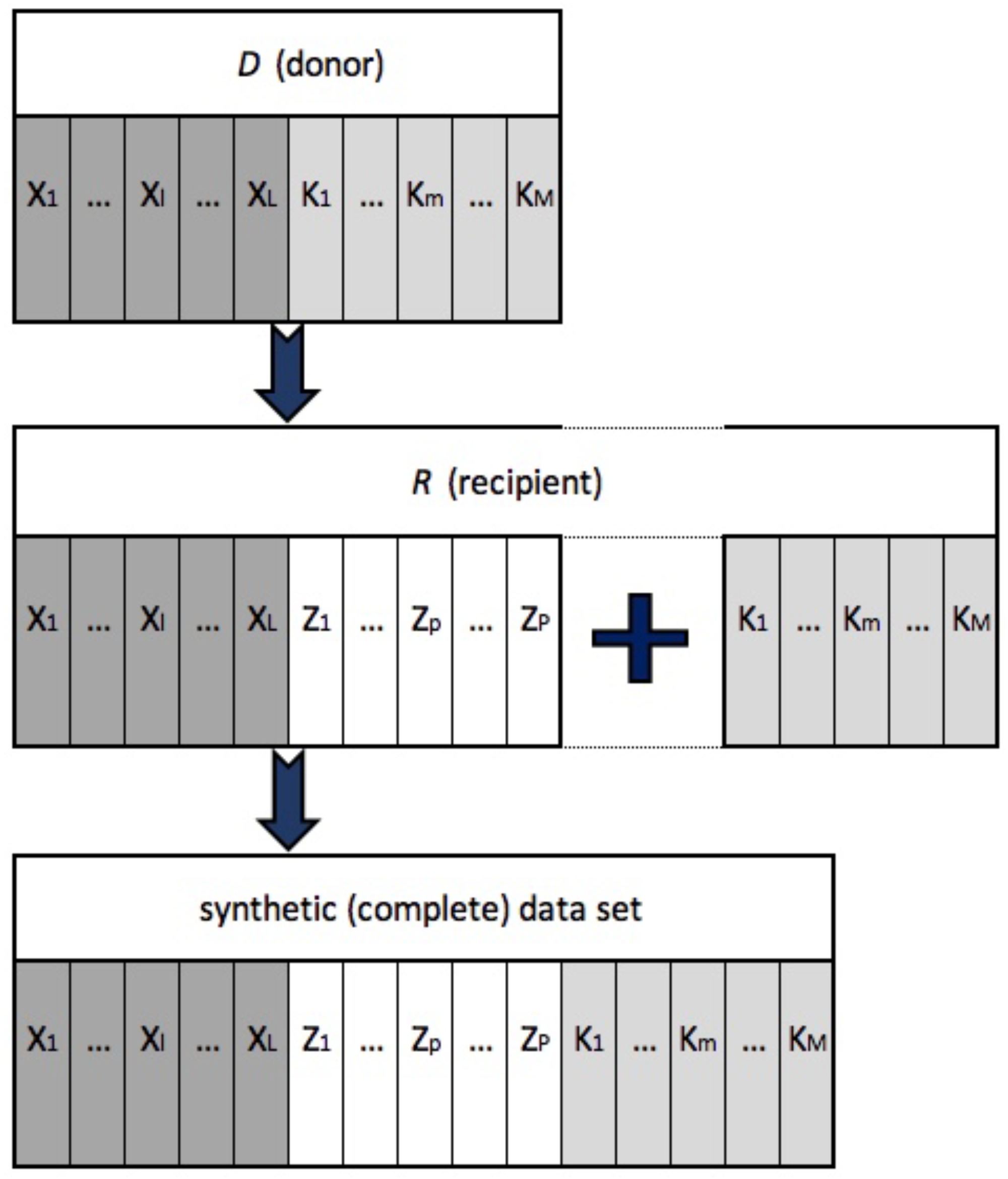
Table 1.
Treatment and control groups in the synthetic (complete) data set “NEW CAP-IRE 2009”.
| T | Frequency | Percent |
|---|---|---|
| 0 | 178 | 62.46 |
| 1 | 107 | 37.54 |
| Total | 285 | 100.00 |
Table 2.
Covariates used for the propensity score (PS) estimation (NEW CAP-IRE 2009 data set). Coef. = coefficients; Std. Err. = Standard Error; z = value of the test statistic; P > |z| = p-value; Conf. Interval = Confidence Interval.
Table 2.
Covariates used for the propensity score (PS) estimation (NEW CAP-IRE 2009 data set). Coef. = coefficients; Std. Err. = Standard Error; z = value of the test statistic; P > |z| = p-value; Conf. Interval = Confidence Interval.
| T | Coef. | Std. Err. | z | P | [95% Conf. Interval] | |
|---|---|---|---|---|---|---|
| owner_agri_edu | −0.476215 | 0.340462 | −1.40 | 0.162 | −1.143509 | 0.191078 |
| owner_edu | 0.115175 | 0.117493 | 0.98 | 0.032 | −0.115107 | 0.345456 |
| legal_status | 0.778176 | 0.303509 | 2.56 | 0.010 | 0.183310 | 1.373043 |
| organic_prod | 0.920301 | 0.424769 | 2.17 | 0.030 | 0.087770 | 1.752832 |
| sfp_ha | −1.015806 | 0.375366 | −2.71 | 0.007 | −1.751510 | −0.280103 |
| sfp_eur | 0.002397 | 0.001040 | 2.30 | 0.021 | 0.000357 | 0.004436 |
| size_esu | 0.000295 | 0.000277 | 1.06 | 0.028 | −0.000249 | 0.000838 |
| uaa_irr | 0.014194 | 0.007912 | 1.79 | 0.073 | −0.001314 | 0.0297015 |
| gfi | −0.000016 | 0.000008 | −2.08 | 0.038 | −0.000032 | −0.000001 |
| ffi | 0.000015 | 0.000008 | 1.92 | 0.054 | −0.000000 | 0.000031 |
| awu_total_input | 0.513978 | 0.183611 | 2.80 | 0.005 | 0.154109 | 0.873847 |
Table 3.
Estimated PS in the region of common support (NEW CAP-IRE 2009 data set). Obs. = number of observations; Std. Dev. = Standard Deviation.
Table 3.
Estimated PS in the region of common support (NEW CAP-IRE 2009 data set). Obs. = number of observations; Std. Dev. = Standard Deviation.
| Percentiles | Smallest | |||
|---|---|---|---|---|
| 1% | 0.155566 | 0.152536 | ||
| 5% | 0.173274 | 0.154019 | ||
| 10% | 0.197719 | 0.155566 | ||
| 25% | 0.240842 | 0.155584 | ||
| 50% | 0.345959 | 0.381021 | ||
| Largest | ||||
| 75% | 0.487506 | 0.894942 | Obs. | 279 |
| 90% | 0.651458 | 0.899009 | Std. Dev. | 0.175115 |
| 95% | 0.750122 | 0.922094 | Variance | 0.030665 |
| 99% | 0.899009 | 0.928727 | Pseudo R | 0.1840 |
Table 4.
Balancing blocks of PS in the region of common support (NEW CAP-IRE 2009 data set).
| Inferior of PS Block | T | Total | |
|---|---|---|---|
| 0 | 1 | ||
| 0.152536 | 15 | 6 | 21 |
| 0.2 | 66 | 24 | 90 |
| 0.3 | 43 | 33 | 76 |
| 0.4 | 35 | 30 | 65 |
| 0.6 | 10 | 8 | 18 |
| 0.8 | 3 | 6 | 9 |
| Total | 172 | 107 | 279 |
Table 5.
Covariates used for the PS estimation using only CAP-IRE 2009.
| T | Coef. | Std. Err. | z | P | [95% Conf. Interval] | |
|---|---|---|---|---|---|---|
| owner_agri_edu | −0.233312 | 0.316948 | −0.74 | 0.462 | −0.854522 | 0.387897 |
| owner_edu | 0.128069 | 0.110731 | 1.16 | 0.247 | −0.088961 | 0.345099 |
| legal_status | 0.916068 | 0.287123 | 3.19 | 0.105 | 0.353318 | 1.478818 |
| organic_prod | 0.914884 | 0.409481 | 2.23 | 0.075 | 0.112316 | 1.717453 |
| ffi | −1.158031 | 0.000003 | −0.68 | 0.497 | −0.000009 | 0.000004 |
Table 6.
Average treatment effect on treated (ATT) estimated on the land_rent_in outcome variable in the synthetic (complete) NEW CAP-IRE 2009 data set. T-stat = test statistic.
Table 6.
Average treatment effect on treated (ATT) estimated on the land_rent_in outcome variable in the synthetic (complete) NEW CAP-IRE 2009 data set. T-stat = test statistic.
| Variable | Sample | Treated | Controls | Difference | Std. Err. | T-stat |
|---|---|---|---|---|---|---|
| land_rent_in | Unmatched | 8.30841 | 7.18539 | 1.12302 | 2.78536 | 0.40 |
| ATT | 8.35577 | 12.31989 | −3.96412 | 2.93514 | −1.35 |
Table 7.
ATT estimated on the ghi outcome variable in the synthetic (complete) NEW CAP-IRE 2009 data set.
Table 7.
ATT estimated on the ghi outcome variable in the synthetic (complete) NEW CAP-IRE 2009 data set.
| Variable | Sample | Treated | Controls | Difference | Std. Err. | T-stat |
|---|---|---|---|---|---|---|
| ghi | Unmatched | 0.18454 | 0.13551 | 0.49028 | 0.26747 | 1.83 |
| ATT | 0.15188 | 0.18839 | −0.03651 | 0.05547 | −0.66 |
© 2018 by the authors. Licensee MDPI, Basel, Switzerland. This article is an open access article distributed under the terms and conditions of the Creative Commons Attribution (CC BY) license (http://creativecommons.org/licenses/by/4.0/).
Share and Cite
MDPI and ACS Style
D’Alberto, R.; Zavalloni, M.; Raggi, M.; Viaggi, D. AES Impact Evaluation With Integrated Farm Data: Combining Statistical Matching and Propensity Score Matching. Sustainability 2018, 10, 4320. https://doi.org/10.3390/su10114320
AMA Style
D’Alberto R, Zavalloni M, Raggi M, Viaggi D. AES Impact Evaluation With Integrated Farm Data: Combining Statistical Matching and Propensity Score Matching. Sustainability. 2018; 10(11):4320. https://doi.org/10.3390/su10114320
Chicago/Turabian StyleD’Alberto, Riccardo, Matteo Zavalloni, Meri Raggi, and Davide Viaggi. 2018. "AES Impact Evaluation With Integrated Farm Data: Combining Statistical Matching and Propensity Score Matching" Sustainability 10, no. 11: 4320. https://doi.org/10.3390/su10114320
Note that from the first issue of 2016, this journal uses article numbers instead of page numbers. See further details here.