A Sustainable Power Plant Control Strategy Based on Fuzzy Extended State Observer and Predictive Control


1
Key Lab of Energy Thermal Conversion and Control of Ministry of Education, Southeast University, Nanjing 210096, China
2
School of Agricultural Engineering and Food Science, Shandong University of Technology, Zibo 255049, China
3
Department of Electrical and Computer Engineering, Baylor University, Waco, TX 76798-7356, USA
*
Author to whom correspondence should be addressed.
Sustainability 2018, 10(12), 4824; https://doi.org/10.3390/su10124824
Submission received: 8 November 2018
/
Revised: 6 December 2018
/
Accepted: 13 December 2018
/
Published: 18 December 2018
(This article belongs to the Collection Power System and Sustainability)
Abstract
:The control of an ultra-supercritical (USC) boiler–turbine power plant is critical in maintaining the safety of the sustainable power grid. However, it is challenging due to the internal nonlinearity, hard manipulation constraints, and widespread uncertainties. To this end, a fuzzy extended state observer (FESO)-based stable fuzzy predictive control (SFPC) approach is developed in this paper. First, the control difficulties of the USC boiler–turbine unit are analyzed. Then, based on a Takagi–Sugeno (T–S) fuzzy model, a new FESO is developed for nonlinear systems to achieve a more precise observation performance. The gain of FESO is determined by solving a series of linear matrix inequalities, while guaranteeing the stability of FESO. Then, by combining the proposed FESO with the SFPC, an integrated FESO–SFPC algorithm is devised. The disturbance rejection ability of the FESO–SFPC algorithm is analyzed theoretically. Simulation results on a 1000 MW USC boiler–turbine power plant model further validate the effectiveness of the proposed method.
1. Introduction
Ultra-supercritical (USC) power plants have been gaining increasing attention in modern coal-fired power industry because of their high efficiency with low emission. A boiler–turbine coordinated control system is of paramount significance in meeting the load demand and maintaining the safety and efficiency of the power grid [1]. Moreover, the USC power plant is now bearing increasing responsibilities in providing flexible power to the grid due to the increasing penetration of intermittent renewables. To achieve a sustainable future for renewable energy, a conventional power plant is required to be able to change its power output rapidly to balance the grid load in the presence of intermittent renewable generation [2].
However, it is extremely challenging to control a USC boiler–turbine unit because of the nonlinearity, the coupling among multi-variables, and the hard constraints on the manipulated variables. To overcome these issues, various control strategies for a boiler–turbine system have been studied, such as robust control [2], optimal control [3], intelligent control [4], sliding model control [5], active disturbance rejection control [6], model predictive control (MPC) [7], etc. The aforementioned methods have significantly improved the performance in some respects but also suffer from some deficiencies. Robust control is often too conservative for the purpose of ensuring the performance in a critical case. The online computation cost of intelligent control methods is huge, which limits their practical application. The chattering phenomenon of the sliding model control will damage the protection of an actuator. On the other hand, MPC is regarded as the most promising control approach because of the ability in dealing with the multi-variable constraint problems explicitly [8,9]. In recent years, MPC has been used in the dynamic stabilization of DC microgrids [10], control of electric vehicles [11], load frequency control [12], and control of DC–DC converters [13], achieving good simulation and experimental results.
Furthermore, some new challenges have appeared in the regulation of a boiler–turbine unit, including time-varying unknown uncertainties caused by the stochastic and intermittent power generation from renewable energy and time-varying unknown disturbances caused by the variation of coal quality. Uncertainties, including parameter perturbations, un-modeled dynamics, and disturbances, always have negative effects on the system’s performance and even threaten the stability of the control system [14,15,16]. Thus, one of the foremost requirements for controllers is to reduce the sensitivity to uncertainties.
To solve the aforementioned problems, reference [17] proposed an adaptive state feedback to handle the unknown uncertainties of the boiler–turbine unit, where the input constraint is however neglected. Reference [18] developed an extended state observer-based fuzzy MPC to overcome the nonlinearity and disturbances simultaneously. However, its compensation action is directly added to the input side, resulting in the destruction of the input constraints and overall optimality. In reference [19], a fuzzy disturbance rejection predictive control approach is proposed; nevertheless, the closed-loop system stability cannot be guaranteed.
In this paper, we aim to propose a control strategy that is able to regulate an input-constrained nonlinear USC boiler–turbine unit to overcome the defects of the existing controls. The major contributions of this paper are summarized as follows:
- (1)
- The nonlinearity of a 1000 MW USC boiler–turbine unit model is analyzed visually by using the V-gap metric.
- (2)
- Based on a Takagi–Sugeno (T–S) fuzzy model, a novel FESO, which is suitable for both single-input–single-output (SISO) and multi-input–multi-output (MIMO) systems, is proposed for the nonlinear system. Compared to the standard extended state observer (ESO), the proposed FESO can achieve a more precise observation performance. The advantages of the FESO are easy to determine by solving a series of linear matrix inequalities, guaranteeing the stability of the FESO.
- (3)
- An integrated FESO–SFPC strategy is devised for input-constrained nonlinear systems with unknown uncertainties, which brings a remarkable performance improvement. The disturbance rejection property of the proposed FESO–SFPC strategy is analyzed theoretically and verified through simulations. Simultaneously, the closed-loop stability is guaranteed.
The remainder of this paper is organized as follows. In Section 2, a 1000 MW USC boiler–turbine unit model is described, and the control difficulties are analyzed. In Section 3, the discrete FESO and FESO–SFPC strategy are established. Simulation results are given in Section 4. Finally, the paper is summarized in Section 5.
Notations: For matrices and , means that is a positive-definite matrix; represents the -dimensional Euclidean norm; and are the inverse and transpose of matrix , respectively; in the matrix represents a symmetric block, for example, ; and represent the zero matrix and the unit matrix, respectively; denotes a block-diagonal matrix; represents the infinite norm of matrix ; is the predicted state value at time based on the current state . For a matrix, if the dimension is not specified, it is considered to have a compatible dimension in order to facilitate algebraic operations.
2. Problem Formulation
2.1. System Description
A USC boiler–turbine unit is an energy-conversion device that transforms the chemical energy of fuel to steam thermal energy. The USC boiler–turbine unit consists of a boiler and a turbine; a schematic diagram of the USC boiler–turbine unit is shown in Figure 1.
The boiler–turbine unit used in this paper represents the dynamics of a 1000 MW coal-fired power plant and has been modeled as a third-order nonlinear mathematical model [20]:
where
The symbols in Equations (1) and (2) for the 1000 MW USC boiler–turbine unit model are listed in Table 1.
The manipulated variables and the rate are constrained by the physical limitations of the actuators:
Hence, an input-constrained nonlinear model can be obtained from (1) and (2):
where , , .
Typical equilibrium operating points of the USC boiler–turbine unit are shown in Table 2.
2.2. Control Difficulties
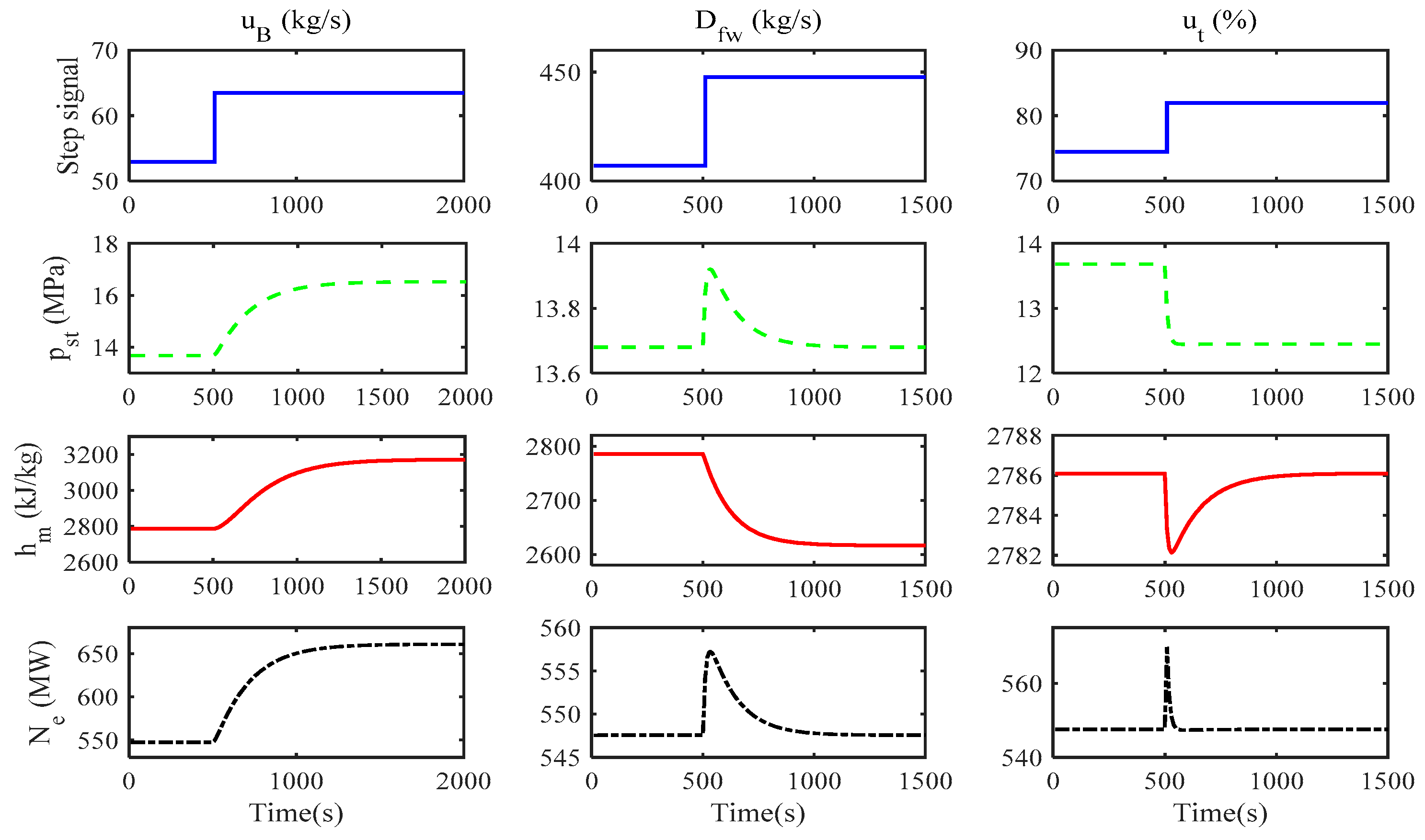
In this section, the control difficulties of the USC boiler–turbine unit will be analyzed in detail. The step response of the USC boiler–turbine unit is shown in Figure 2. From this figure, we can easily conclude that the USC boiler–turbine unit presents a strong coupling among multi-variables and has great inertia.
To quantitatively measure the nonlinearity of the USC boiler–turbine unit, the Vinnicombe gap (V-gap) metric [21,22] between two linearized systems is used, which is defined as
where and are two linear models obtained by linearization at any two operating points of the nonlinear model (1), and and are directed gaps between the linear systems and . Using normalized coprime factorizations, these two linear systems can be represented as and . Then, the directed gap can be calculated by
where is a matrix parameter which has finite H-infinity norm.
For the USC boiler–turbine unit, the linearized model at the operating point #6 in Table 2 is selected as the nominal model. The nonlinearity investigation results are shown in Figure 3. The results indicate that the disturbance between two linearized systems increases as the distance between the operating points increases. Therefore, we can reach the conclusion that the USC boiler–turbine unit has a strong nonlinearity.
On the basis of the aforementioned analysis, the control difficulties mainly consist of great inertia, strong coupling, strong nonlinearity, input constraints, as well as unknown uncertainties.
3. Fuzzy ESO-Based Stable Fuzzy Predictive Control
In this section, a novel T–S fuzzy model-based FESO is proposed, and the stability of the FESO is proved. Then, based on the proposed FESO, an integrated FESO–SFPC strategy is proposed. In the end, the disturbance rejection property of the proposed strategy is analyzed theoretically.
3.1. Fuzzy Extended State Observer
The performance of the ESO-based control systems depends upon the accuracy of the state and the uncertainty estimation [23,24,25,26]. To this end, a novel FESO is developed in this section.
The T–S fuzzy models are extensively employed to represent nonlinear systems [27,28,29]. A discrete affine T–S fuzzy model is used to capture the dynamics of the USC boiler–turbine system:
IF is and is , then
where denotes the -th fuzzy inference rule, is the number of fuzzy rules, represents some measurable variables, represents fuzzy sets, denotes the state variable, is the output variable, is the input variable, represents the uncertainties, including plant–model mismatches and all disturbances, and represents the -th local model of the fuzzy system.
By using a singleton fuzzifier, the product inference, and the center-average defuzzifier, the fuzzy model (7) can be expressed as follows:
where , , , , , , represent the normalized membership function of the inferential fuzzy set , , and .
Assumption 1.
Disturbance is unknown at each time constant but it is bounded.
Assumption 2.
The output trajectory reference and the corresponding desired reference input are known.
The new augmented variables
are introduced into the system (7), where is the difference of a disturbance .
Combining (7) and (9), a novel extended state-space model can be written as
where is the extended state vector, , , , , and are system matrices.
In order to obtain the estimation of the state variables of the extended state-space model (10), the following FESO is designed:
where is the estimation of , and is the observer gain to be designed.
Defining the extended state estimation error , then one has the following observer error dynamic equation:
Theorem 1.
The observer error dynamic system (12) is stable if there exist positive symmetric matrix, matrix, and matrix satisfying the following set of linear matrix inequalities (LMIs):
whereis a given positive matrix parameter. Thus, the FESO gain is.
Proof.
The demonstration of the theorem is given in Appendix A. □
Remark 1.
The convergence rate of the FESO is adjusted by changing the norm of the matrix.
3.2. Fuzzy ESO-Based Stable Fuzzy Predictive Control
To eliminate the effect of unknown uncertainties, a constrained targets calculator is used to determine the steady-state and input target value (, ) by solving the following quadratic programing problem at each sampling time :
where and are the desired input and output set points, is the input constraints.
When the steady-state set point (, ) is obtained, one has
Subtracting system (16) from system (7) yields
where , , , and .
Then, we can use the following nominal model of system (17) as the prediction model
where denotes the predicted state of the plant at time , the future control move at time , the future output at time .
The objective is to minimize the infinite horizon objective function
subject to
where
with and are the symmetric positive definite weighting matrices for output and input variables, respectively.
We aim at finding a state feedback control law
that minimizes the objection function (19).
We define a quadratic function
Supposing satisfies the following inequality
Summing (24) from to , and providing , it follows that
Obviously, (19) is equivalent to
According to Schur Complement Lemma, (25), (24), and (20) can be transformed to (29), (30) and (31), (32).
Summarizing the above arguments, we can obtain the following theorem.
Theorem 2.
For the discrete affine T–S fuzzy model (7) under input constraintwith the FESO (11), whose observer gain is determined by LMIs (13) and target generation procedure (14) and (15), if there exist a series of symmetric positive matricesand matrices, such that following LMI is feasible
subject to (29)–(32), then, at every sampling time, by minimizing the upper bound of the infinite horizon objective function, a control action
is applied to track the reference, while guaranteeing the stability of the closed-loop system and satisfying the input constraints, and
where.
Remark 2.
The equality (29) guarantees that the infinite horizon objective function is minimum at sampling time. The equality (30) guarantees the closed-loop stability. Input constraint is ensured by (31) and (32).
On the basis of the proposed FESO strategy, a FESO-based SFPC algorithm is summarized in Algorithm 1.
| Algorithm 1: Proposed FESO–SFPC algorithm. |
| 1: Initialize: At , Initialize system states , inputs and observer states ; |
| 2: while do |
| 3: Solve problem (27) online with estimated states to obtain the optimal control input ; |
| 4: Apply the optimal control input to the system; |
| 5: Measure the current output ; |
| 6: Estimate based on , and by the proposed FESO (11); |
| 7: k = k + 1; |
| 8: end while |
| is the final time of running the algorithm. |
The schematic diagram of the proposed FESO–SFPC is shown in Figure 4.
3.3. Disturbance Rejection Analysis
Theorem 3.
Supposing thatis bounded and has a constant valve at the steady state, then, and, where c is a constant. Ifis observable, with FESO (11), target generation procedure (14) and (15), and the control law (28), unknown uncertainties can be removed from the output channels in steady state.
Proof.
The demonstration of the theorem is given in Appendix A. □
4. Simulation Results and Discussions
In this section, the FESO–SFPC strategy is applied to control the input-constrained nonlinear USC boiler–turbine unit model with uncertainties and disturbances. First, the T–S fuzzy model of the boiler–turbine system is established. Then, four simulation scenarios are presented to evaluate the proposed FESO–SFPC strategy.
4.1. Modeling of the Boiler–Turbine System
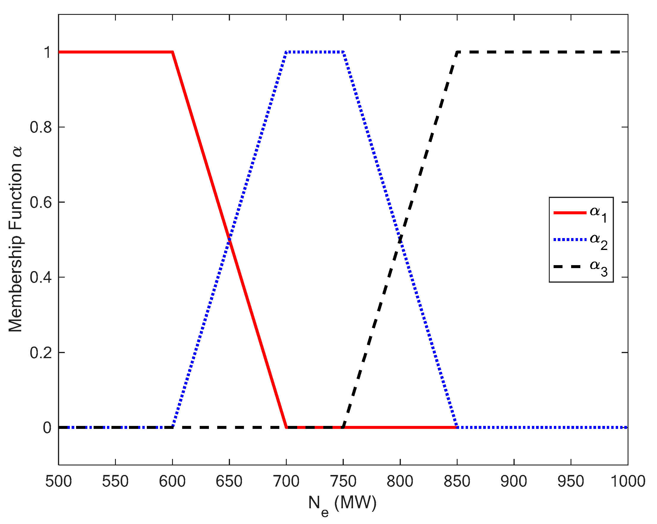
Using the Taylor series expansion, selecting power as the switching variable and choosing the membership function shown in Figure 5, we can easily get the following T–S fuzzy model
where , , , . Matrices are given in Appendix B.
4.2. Performance Evaluations and Discussions
The turning parameters of the proposed FESO–SFPC for the USC boiler–turbine unit are set as follows: the sample time , the weighting matrices , , the coefficient matrices , , the observer coefficient . Then, use Theorem 1 to get the gain of the FESO as follows:
For comparison, two additional controllers are tested on the USC boiler–turbine system under the same design parameters:
4.2.1. Simulation of Disturbance Rejection
In order to verify the disturbance rejection property of the three controllers, three simulation scenarios are designed. We suppose that the USC boiler–turbine unit operates at the operating point #5 (22.54MPa, 2701.3kJ/kg, 901.49MW) in Table 2. Then, the unknown disturbances are added to the input in three different forms, i.e., step-type disturbance, ramp-type disturbance, and curve-type disturbance:
- Case 1:
- A step-type disturbance on the turbine throttle valve .
- Case 2:
- A ramp-type disturbance on the water input channel .
- Case 3:
- A curve-type disturbance on the fuel input channel .
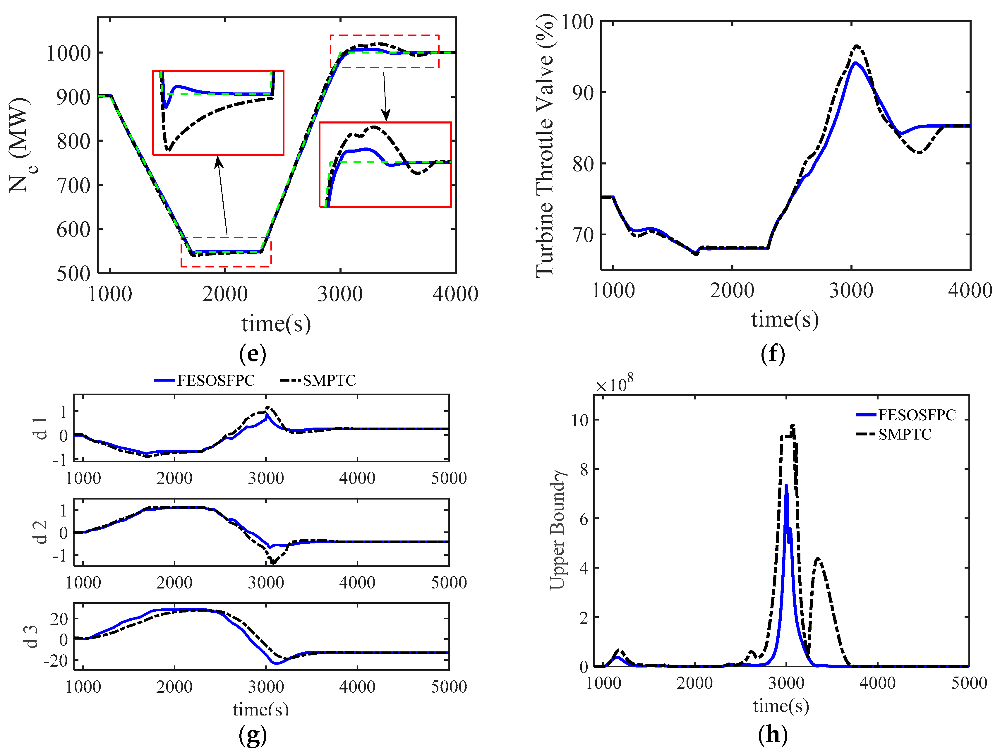
Figure 8 shows the response result in Case 1. (a), (c) and (e) of Figure 8 show the output of the system under the action of the three controllers, where it can be seen that all three controllers can eliminate the effect of the step-type disturbance, but the proposed FESO–SFPC has the best performance. (b), (d) and (f) of Figure 8 show the output of the three controllers, all of which satisfy the actuator constraints. Figure 8g shows the observed disturbances, and the proposed method has a faster disturbance observation speed. It is worth noting that the disturbances in Figure 8g are not true disturbances and can be understood as the sum of all uncertainties. It can be seen from Figure 8h that the under the adjustment of the two controllers becomes 0 with time, which indicates that the closed-loop system has converged. In addition, the proposed method converges faster, which indicates that the performance of the proposed method is better. Compared with ESO–FMPC, the proposed method not only has a better performance, but also ensures the stability of the closed-loop system.
Case 2 is designed to test the performance of the controller for ramp-type disturbance rejection. It can be seen from Figure 9 that the SMPTC method cannot compensate for the ramp-type disturbance. Both FESO–SFPC and ESO–FMPC methods can offset the ramp-type interference. However, the ESO–FMPC method has a large overshoot and does not guarantee the stability of the closed-loop system.
It can be seen from Figure 10 that when the curve-type disturbance occurs at the input end, the control performance of the SMPTC drops sharply, but the proposed method can still achieve a better control and is superior to the ESO–FMPC algorithm.
4.2.2. Simulation on Load Tracking
In addition, Case 4 is devised to test the property of load tracking with unknown time-varying uncertainties. The USC boiler–turbine unit operates at the operating point #5 (22.54MPa, 2701.3kJ/kg, 901.49MW) in Table 2 and then ramps to the operating point #1 (13.68MPa, 2786.1kJ/kg, 547.56MW). After keeping constant for a period, it ramps to the operating point #6 (22.6MPa, 2698kJ/kg, 1000MW). Finally, it arrives at a steady state. Meanwhile, continuous uncertainties are added into the nonlinear model of the USC boiler–turbine unit by making the output in nonlinear model change according to the following function, which is unknown to the controller:
Figure 11 shows the response under Case 4. The closed-loop system is diverged under the control of the ESO–FMPC, so the curve is not drawn in Figure 11. The main reason is that feed forward destroys the stability of the system. Compared with the SMPTC method, the FESO–SFPC strategy has a shorter recovery time and a smaller overshoot. From an overall perspective, the overall performance of the proposed FESO–SFPC strategy is better than those of the ESO–FMPC and SMPTC methods.
The integrated absolute errors (IAEs) of the controllers in Case 1 to Case 4 are listed in Table 3. In the four cases, the proposed method has the smallest IAE.
4.3. Parameter Effects on Control Performance
The adjustment parameters of the proposed algorithm are , and . The effects of the three adjustment parameters on the performance of the closed-loop system were analyzed by changing the parameters in simulation. However, these parameters do not have a large influence on the closed-loop system when they vary within a certain range, which also indicates that the proposed controller’s adjustment parameters are easy to set.
5. Conclusions
The conventional coal-fired power plant is now facing more challenges because of the increasing penetration of intermittent renewables. In order to solve the uncertainty of the ultra-supercritical boiler–turbine unit, an SFPC method based on FESO is adopted. The FESO is designed to estimate and compensate the total disturbance. The SFPC is used to handle the constraints and coupling, realizing operation purpose optimally. The stability and disturbance rejection performance are theoretically analyzed. The simulation results show that, compared to SMPTC and ESO–FMPC, the proposed FESO–SFPC strategy has significant ability to deal with uncertainties as a result of the observation performance of the FESO. The fast, stable, and flexible load-tracking performance of the power plant depicts a promising prospect for the proposed strategy in facilitating the sustainability of the future power grid.
Author Contributions
All authors collectively conceived the research and carried out the analysis. C.C. led the simulation and paper writing with contributions and guidance from L.P., S.L., L.S., and K.Y.L.
Funding
This work was supported by the National Natural Science Foundation of China under Grants 51576040, 51606113, and 51706093, and the Natural Science Foundation of Jiangsu Province, China, under Grant BK20170686.
Conflicts of Interest
The authors declare no conflict of interest.
Appendix A. Proof of Theorem 1 and Theorem 3
Proof of Theorem 1.
Consider a candidate Lyapunov function defined as
The difference of candidate Lyapunov function (A1) along a trajectory of system (12) is given by
In order to adjust the convergence rate of the FESO, suppose satisfies the inequality
Since , the above inequality (A3) is satisfied if
According to the Schur Complement Lemma, the above inequality (A4) is satisfied if
Defining , we can achieve
from (A5) by multiplying (A6) from the left by and, from the right, by and using the equality .
Therefore, which means that the observer error system (12) is stable, and thus Theorem 1 is proved. □
Proof of Theorem 3.
Supposing that and bespeak the estimates of the system steady state and lumped disturbance, respectively, and are the steady-state control inputs and outputs. Thus, by FESO (11), we have
in which , are block matrices of , meeting .
It has been proved by [31,32], that the FESO gain is full-rank, while the number of the disturbances are equal to the number of outputs. Thus, from (A8) and (A7), we get
If there exists a feasible result to the target generation procedure (14) and (15), we have
Subtracting (A12) from (A10) yields
Then, from (28), we can get
Then, one obtains from (A13) and (A14)
As the closed-loop system has been ensured to be stable, the eigenvalue of is within the unit circle, thus the only solution of (A15) is .
Subtracting (A11) from (A9) yields
On the basis of the target generation procedure (14) and (15), we have at steady state; hence, unknown uncertainties can be removed from the output channels in steady state. □
Appendix B. Local Linear Models for T–S Fuzzy Model
; ;
; ;
; ;
; ;
; ;
; .
References
- Wu, X.; Shen, J.; Li, Y.; Lee, K.Y. Steam power plant configuration, design, and control. Wiley Interdiscip. Rev. Energy Environ. 2015, 4, 537–563. [Google Scholar] [CrossRef]
- Sun, L.; Hua, Q.; Shen, J.; Xue, Y.; Li, D.; Lee, K.Y. Multi-objective optimization for advanced superheater steam temperature control in a 300 MW power plant. Appl. Energy 2017, 208, 592–606. [Google Scholar] [CrossRef]
- Li, Y.; Shen, J.; Lee, K.Y.; Liu, X. Offset-free fuzzy model predictive control of a boiler-turbine system based on genetic algorithm. Simul. Model. Pract. Theory 2012, 26, 77–95. [Google Scholar] [CrossRef]
- Ma, L.; Lee, K.Y.; Wang, Z. Intelligent coordinated controller design for a 600 MW supercritical boiler unit based on expanded-structure neural network inverse models. Control Eng. Pract. 2016, 53, 194–201. [Google Scholar] [CrossRef]
- Ghabraei, S.; Moradi, H.; Vossoughi, G. Multivariable robust adaptive sliding mode control of an industrial boiler-turbine in the presence of modeling imprecisions and external disturbances: A comparison with type-I servo controller. ISA Trans. 2015, 58, 398–408. [Google Scholar] [CrossRef]
- Sun, L.; Hua, Q.; Li, D.; Pan, L.; Xue, Y.; Lee, K.Y. Direct energy balance based active disturbance rejection control for coal-fired power plant. ISA Trans. 2017, 70, 486–493. [Google Scholar] [CrossRef]
- Ławryńczuk, M. Nonlinear predictive control of a boiler-turbine unit: A state-space approach with successive on-line model linearisation and quadratic optimisation. ISA Trans. 2017, 67, 476–495. [Google Scholar] [CrossRef]
- Mayne, D.Q. Model predictive control: Recent developments and future promise. Automatica 2014, 50, 2967–2986. [Google Scholar] [CrossRef]
- Xi, Y.-G.; Li, D.-W.; Lin, S. Model Predictive Control—Status and Challenges. Acta Autom. Sin. 2013, 39, 222–236. [Google Scholar] [CrossRef]
- Vafamand, N.; Khooban, M.H.; Dragičević, T.; Blaabjerg, F. Networked fuzzy predictive control of power buffers for dynamic stabilization of DC microgrids. IEEE Trans. Ind. Electron. 2019, 66, 1356–1362. [Google Scholar] [CrossRef]
- Khooban, M.H.; Vafamand, N.; Niknam, T.; Dragicevic, T.; Blaabjerg, F. Model-predictive control based on Takagi-Sugeno fuzzy model for electrical vehicles delayed model. IET Electr. Power Appl. 2017, 11, 918–934. [Google Scholar] [CrossRef]
- Khooban, M.-H.; Dragicevic, T.; Blaabjerg, F.; Delimar, M. Shipboard microgrids: A novel approach to load frequency control. IEEE Trans. Sustain. Energy 2018, 9, 843–852. [Google Scholar] [CrossRef]
- Mardani, M.M.; Khooban, M.H.; Masoudian, A.; Dragičević, T. Model Predictive Control of DC-DC Converters to Mitigate the Effects of Pulsed Power Loads in Naval DC Microgrids. IEEE Trans. Ind. Electron. 2018. [Google Scholar] [CrossRef]
- Chen, W.H.; Yang, J.; Guo, L.; Li, S. Disturbance-Observer-Based Control and Related Methods—An Overview. IEEE Trans. Ind. Electron. 2016, 63, 1083–1095. [Google Scholar] [CrossRef] [Green Version]
- Gao, Z. On the centrality of disturbance rejection in automatic control. ISA Trans. 2014, 53, 850–857. [Google Scholar] [CrossRef] [Green Version]
- Li, S. Disturbance Observer-Based Control—Methods and Applications; CRC Press, Inc.: Boca Raton, FL, USA, 2014. [Google Scholar]
- Pan, L.; Luo, J.; Cao, C.; Shen, J. L1 adaptive control for improving load-following capability of nonlinear boiler-turbine units in the presence of unknown uncertainties. Simul. Model. Pract. Theory 2015, 57, 26–44. [Google Scholar] [CrossRef]
- Zhang, F.; Wu, X.; Shen, J. Extended state observer based fuzzy model predictive control for ultra-supercritical boiler-turbine unit. Appl. Therm. Eng. 2017, 118, 90–100. [Google Scholar] [CrossRef]
- Zhang, F.; Wu, X.; Shen, J. Fuzzy disturbance rejection predictive control of ultra-supercritical once-through boiler-turbine unit. J. Southeast Univ. 2017, 33, 53–58. [Google Scholar]
- Liu, J.Z.; Yan, S.; Zeng, D.L.; Hu, Y.; Lv, Y. A dynamic model used for controller design of a coal fired once-through boiler-turbine unit. Energy 2015, 93, 2069–2078. [Google Scholar] [CrossRef]
- Georgiou, T.T. On the computation of the gap metric. In Proceedings of the 27th IEEE Conference on Decision and Control, Austin, TX, USA, 7–9 December 1988; pp. 1360–1361. [Google Scholar]
- Sun, L.; Li, D.; Lee, K.Y. Enhanced decentralized PI control for fluidized bed combustor via advanced disturbance observer. Control Eng. Pract. 2015, 42, 128–139. [Google Scholar] [CrossRef]
- Madoński, R.; Herman, P. Survey on methods of increasing the efficiency of extended state disturbance observers. ISA Trans. 2015, 56, 18–27. [Google Scholar] [CrossRef] [PubMed]
- Sun, L.; Shen, J.; Hua, Q.; Lee, K.Y. Data-driven oxygen excess ratio control for proton exchange membrane fuel cell. Appl. Energy 2018, 231, 866–875. [Google Scholar] [CrossRef]
- Sun, L.; Wu, G.; Xue, Y.; Shen, J.; Li, D.; Lee, K.Y. Coordinated Control Strategies for Fuel Cell Power Plant in a Microgrid. IEEE Trans. Energy Convers. 2018, 33, 1–9. [Google Scholar] [CrossRef]
- Sun, L.; Hua, Q.; Shen, J.; Xue, Y.; Li, D.; Lee, K.Y. A Combined Voltage Control Strategy for Fuel Cell. Sustainability 2017, 9, 1517. [Google Scholar] [CrossRef]
- Chiu, S.L. Fuzzy model identification based on cluster estimation. J. Intell. Fuzzy Syst. 1994, 2, 267–278. [Google Scholar]
- Wu, L.; Su, X.; Shi, P.; Qiu, J. A new approach to stability analysis and stabilization of discrete-time TS fuzzy time-varying delay systems. IEEE Trans. Syst. Man Cybern. Part B 2011, 41, 273–286. [Google Scholar] [CrossRef] [PubMed]
- Tseng, C.-S.; Chen, B.-S.; Uang, H.-J. Fuzzy tracking control design for nonlinear dynamic systems via TS fuzzy model. IEEE Trans. Fuzzy Syst. 2001, 9, 381–392. [Google Scholar] [CrossRef]
- Wu, X.; Shen, J.; Li, Y.; Lee, K.Y. Fuzzy modeling and stable model predictive tracking control of large-scale power plants. J. Process Control 2014, 24, 1609–1626. [Google Scholar] [CrossRef]
- Zhang, T.; Feng, G.; Zeng, X.J. Output tracking of constrained nonlinear processes with offset-free input-to-state stable fuzzy predictive control. Automatica 2009, 45, 900–909. [Google Scholar] [CrossRef]
- Muske, K.R.; Badgwell, T.A. Disturbance modeling for offset-free linear model predictive control. J. Process Control 2002, 12, 617–632. [Google Scholar] [CrossRef]
Figure 1.
Schematic diagram of an ultra-supercritical (USC) boiler-turbine unit.

Figure 2.
Open-loop step response of the boiler–turbine unit.

Figure 3.
Distribution of nonlinearity of the system.

Figure 4.
The fuzzy extended state observer (FESO)–stable fuzzy predictive control (SFPC) schematic.
Figure 4.
The fuzzy extended state observer (FESO)–stable fuzzy predictive control (SFPC) schematic.

Figure 5.
Membership function. Switching variables, , , and are, respectively, low-, medium-, and high-power.
Figure 5.
Membership function. Switching variables, , , and are, respectively, low-, medium-, and high-power.

Figure 6.
Input used in the fuzzy model verification.

Figure 7.
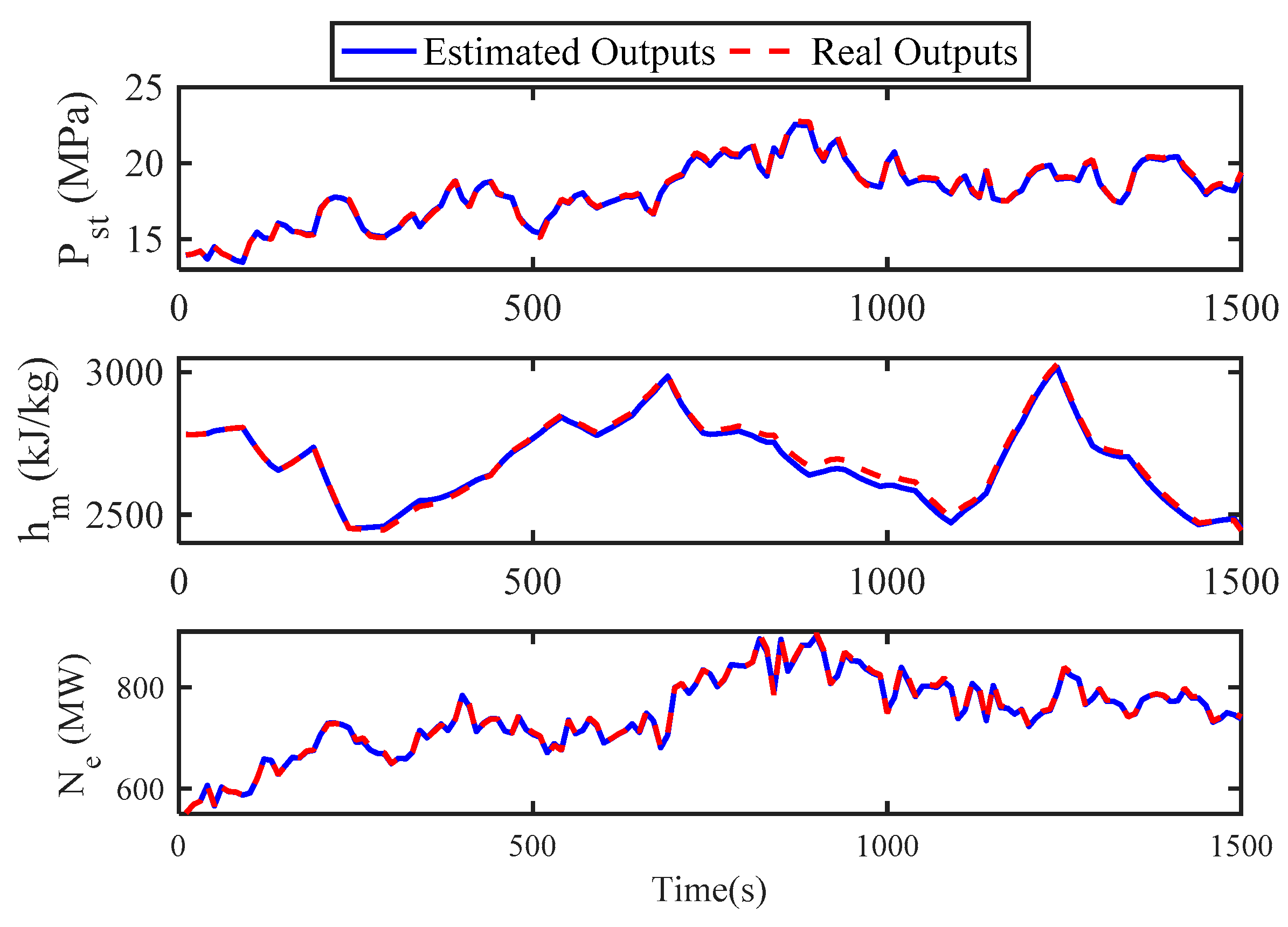
Fuzzy model verification.

Figure 8.
Case 1: Responses to a step-type disturbance applied to the turbine throttle valve. (a,c,e) Output disturbance response; (b,d,f) Input disturbance response; (g) Disturbance estimation; (h) Upper bound of the objective function, showing the performance of the controllers; SMPTC: stable model predictive tracking controller; ESO–FMPC: ESO-based fuzzy model predictive control; FESO-SFPC: fuzzy ESO-based stable fuzzy predictive control.

Figure 9.
Case 2: Responses to a ramp-type disturbance applied to the water input channel. (a,c,e) Output disturbance response; (b,d,f) Input disturbance response; (g) Disturbance estimation; (h) Upper bound of the objective function, showing the performance of the controllers.
Figure 9.
Case 2: Responses to a ramp-type disturbance applied to the water input channel. (a,c,e) Output disturbance response; (b,d,f) Input disturbance response; (g) Disturbance estimation; (h) Upper bound of the objective function, showing the performance of the controllers.

Figure 10.
Case 3: Responses to a ramp-type disturbance applied to the fuel input channel. (a,c,e) Output disturbance response; (b,d,f) Input disturbance response; (g) Disturbance estimation; (h) Upper bound of the objective function, showing the performance of the controller.
Figure 10.
Case 3: Responses to a ramp-type disturbance applied to the fuel input channel. (a,c,e) Output disturbance response; (b,d,f) Input disturbance response; (g) Disturbance estimation; (h) Upper bound of the objective function, showing the performance of the controller.

Figure 11.
Case 4: Load tracking. (a,c,e) Output disturbance response; (b,d,f) Input disturbance response; (g) Disturbance estimation; (h) Upper bound of the objective function, showing the performance of the controller.
Figure 11.
Case 4: Load tracking. (a,c,e) Output disturbance response; (b,d,f) Input disturbance response; (g) Disturbance estimation; (h) Upper bound of the objective function, showing the performance of the controller.


Table 1.
Symbols in the equations relative to the 1000 MW USC boiler-turbine unit model.
| Parameter | Representation | Unit |
|---|---|---|
| Pulverized coal flow rate that enters the boiler | kg/s | |
| Separator steam pressure | MPa | |
| Enthalpy | kJ/kg | |
| Throttle steam pressure | MPa | |
| Separator steam enthalpy | kJ/kg | |
| Active electric power | MW | |
| Fuel flow rate | kg/s | |
| Feed water flow rate | kg/s | |
| Turbine throttle valve opening | % |
Table 2.
Equilibrium operating points of the USC boiler–turbine unit.
| #1 | 13.68 | 2786.1 | 547.56 | 52.9 | 407.03 | 74.47 |
| #2 | 16.3 | 2751.5 | 650 | 62.48 | 492.31 | 74.25 |
| #3 | 18.23 | 2729 | 728.33 | 69.77 | 558.50 | 74.56 |
| #4 | 20.0 | 2710.0 | 800.0 | 76.422 | 619.97 | 74.88 |
| #5 | 22.54 | 2701.3 | 901.49 | 85.81 | 702.04 | 75.28 |
| #6 | 22.6 | 2698.0 | 1000 | 94.89 | 780.20 | 83.3 |
Table 3.
Integrated absolute errors (IAE) under Cases 1–4.
| Case | Method | IAE (pst) | IAE (hm) | IAE (Ne) |
|---|---|---|---|---|
| Case 1 | FESO–SFPC | 18.8 | 80.6 | 271.5 |
| ESO–FMPC | 63.7 | 846.6 | 1350.7 | |
| SMPTC | 31.2 | 99.4 | 316.6 | |
| Case 2 | FESO–SFPC | 0.4 | 2.6 | 9.8 |
| ESO–FMPC | 12.5 | 314.7 | 490.7 | |
| SMPTC | 0.5 | 3.1 | 11.3 | |
| Case 3 | FESO–SFPC | 0.51 | 2.2 | 8.9 |
| ESO–FMPC | 14.9 | 384.9 | 582.5 | |
| SMPTC | 2.2 | 11.7 | 19.2 | |
| Case 4 | FESO–SFPC | 131.1 | 264.7 | 829.5 |
| SMPTC | 1036.6 | 5009.6 | 9286.8 |
© 2018 by the authors. Licensee MDPI, Basel, Switzerland. This article is an open access article distributed under the terms and conditions of the Creative Commons Attribution (CC BY) license (http://creativecommons.org/licenses/by/4.0/).
Share and Cite
MDPI and ACS Style
Chen, C.; Pan, L.; Liu, S.; Sun, L.; Lee, K.Y. A Sustainable Power Plant Control Strategy Based on Fuzzy Extended State Observer and Predictive Control. Sustainability 2018, 10, 4824. https://doi.org/10.3390/su10124824
AMA Style
Chen C, Pan L, Liu S, Sun L, Lee KY. A Sustainable Power Plant Control Strategy Based on Fuzzy Extended State Observer and Predictive Control. Sustainability. 2018; 10(12):4824. https://doi.org/10.3390/su10124824
Chicago/Turabian StyleChen, Chen, Lei Pan, Shanjian Liu, Li Sun, and Kwang Y. Lee. 2018. "A Sustainable Power Plant Control Strategy Based on Fuzzy Extended State Observer and Predictive Control" Sustainability 10, no. 12: 4824. https://doi.org/10.3390/su10124824
Note that from the first issue of 2016, this journal uses article numbers instead of page numbers. See further details here.