The Impact of Socio-Economic Indicators on Sustainable Consumption of Domestic Electricity in Lithuania

1
Department of Management and Human Resources Development, Alexander Dubcek University, 91150 Trencin, Slovakia
2
School of Economics and Business, Kaunas University of Technology, 44239 Kaunas, Lithuania
*
Author to whom correspondence should be addressed.
Sustainability 2018, 10(2), 162; https://doi.org/10.3390/su10020162
Submission received: 26 December 2017
/
Revised: 13 January 2018
/
Accepted: 17 January 2018
/
Published: 23 January 2018
(This article belongs to the Special Issue Sustainable Electric Power Systems Research)
Abstract
:Lithuania is one of the EU Member States, where the rate of energy consumption is comparatively low but consumption of electricity has been gradually increasing over the last few years. Despite this trend, households in only three EU Member States consume less electricity than Lithuanian households. The purpose of this research is to analyse the impact of socio-economic factors on the domestic electricity consumption in Lithuania, i.e., to establish whether electricity consumption is determined by socio-economic conditions or population’s awareness to save energy. Cointegration analysis, causality test and error-correction model were used for the analysis. The results reveal that there is a long run equilibrium relationship between residential electricity consumption per capita and GDP at current prices as well as the ratio of the registered unemployed to the working-age population. In consequence, the results of the research propose that improvement of living standards for Lithuanian community calls for the necessity to pay particular attention to the promotion of sustainable electricity consumption by providing consumers with appropriate information and feedback in order to seek new energy-related consumption practices.
1. Introduction
Sustainable energy development and assessment are the topical issues in the latest research on the field of energy. The importance of energy lies in its wide applicability and indispensability. Energy, as the concerning issue for people around the world, is an inevitable component of their daily lives [1]. Social and economic development of modern societies is based on energy [2]. Energy is the key contributor to poverty relief, the increase in human welfare and improvement of living standards. Energy is placed in the middle of triangle among the nature, society and economy; it is treated as an essential element of global progress [3]. Growth of population and economics requires even the increasing demand of energy every year. As the resources are limited and unreasonable consumption of resources has a negative impact on environment, each of us must follow the principles of sustainable energy consumption.
In recent years, much work has been done to make energy more sustainable, i.e., economic and efficient, clean and secure [4]. Many discussions and debates about sustainable development take place in governments as well non-government and academic circles. Hence, sustainable development has become a major focus of the national and international economic, social and environmental agendas [5,6,7]. Investment in energy efficiency has a potential to contribute to economic growth, employment, innovation and reduction of fuel poverty in households and therefore makes a positive contribution to economic, social and territorial cohesion [8].
In the 21-st century, the world confronts the challenge of converting its base of fossil fuels energy to sustainable energy resources. The major interest is to reach a sustainable energy balance in order to avoid the negative effects of global warming and significant economic problems, which are faced when the resources of oil and gas are rapidly declining and becoming too expensive to use [2,9].
As transport and heating are getting climate-friendlier, the environmental effect of energy consumption is increasingly determined by electricity. The degree of electrification measured in terms of the share of electric energy in the final energy mix is predicted to sharply increase by 2050. The increase in electric energy efficiency is considered to result in smaller amounts of electricity required for fulfillment of a given demand for power and light. However, the demand is predicted to significantly increase in account of the growth economies and electrification of transport and heating. With reference to the forecasts of the World Energy Council, world electricity consumption will have increased twice by 2050.
According to Filippini et al. [10], Yohanis et al. [11] and other researchers, the residential sector of the EU holds a relatively high potential for energy savings. With reference to the data of Eurostat for the 10-year period from 2005 to 2015, consumption of electricity by households fell by 0.9% in EU-28. The decrease in electricity consumption in individual states was even faster: consumption of electricity in Belgian households decreased by 27.6%, while in British households it decreased by 14%. Nevertheless, despite the general trends of decrease, total figures of household electricity consumption rose in the biggest part (18) of the EU Member States, generally by less than 20%. The largest expansions were recorded for Romania (31.0%) and Lithuania (23.0%).
As a member of the EU, Lithuania develops various programs to insure the effective use of energy. Lithuanian household energy accounts for about 30% of all the energy consumed in the country. Consumption of the biggest part of energy sources has been decreasing over the last decade but consumption of electricity has still been rising despite all the exhortations to save energy. The purpose of this research is to analyse the impact of socio-economic factors on the domestic electricity consumption in Lithuania. The paper seeks to reveal the trends of household energy consumption in Lithuania and to establish the main socio-economic factors that it depends on.
The results of the research might help to develop the measures that would promote electricity saving in the country in order to achieve the aims of the strategy Energy 2020 [12]. Furthermore, if electricity consumption is determined by socio-economic conditions and electricity saving constitutes the major concern for the reduction of pollution, then Lithuanian government must turn to the appropriate programs, including financial incentives, changes in tax legislation and etc. and to information campaigns that assist to change resident behaviour and encourage households to use power saving features in all electrical appliances. On the other hand, the financial and living conditions and population’s awareness to save energy in Lithuania change and it raises interesting discussion topics and further research issues from the sustainability perspective. Finally, there is more empirical work to be done to explore whether and how the changes of socio-economic factors and residents’ behaviour are able to reconfigure everyday life practices and household electricity consumption. It would be interesting to investigate what do more sustainable energy-consuming practices in different countries look like and how the changes of socio-economic factors and resident behaviour influence household electricity consumption in other communities.
The remainder of this paper has been organized as follows: at first, the analysis of the literature on sustainable usage of electricity and general energy has been conducted by emphasizing the importance of energy saving in households and highlighting the main factors that affect electricity consumption in households; next, the analysis of energy and electricity consumption in Lithuania has been conducted. Finally, the impact of particular economic and social indicators on electricity consumption in Lithuanian households has been researched.
2. Materials and Methods
2.1. Literature Review
2.1.1. The Issues of Sustainable Use of Energy
Energy plays a vital role in economic development. Many studies have sought to find the causality between energy and economic growth but still no consensus has emerged. Chontanawat et al. [13] tested for causality between energy and GDP for over 100 countries. Causality from energy to GDP is found to be more prevalent in the developed OECD countries in comparison to the developing non-OECD countries. This implies that a policy to reduce energy consumption aimed at reducing emissions is likely to have a greater impact on GDP of the developed countries rather than on GDP of the developing world. Lee [14], who investigated the causal relationship between energy consumption and GDP in 18 developing countries by employing the data for the period 1975 to 2001, showed that long-run and short-run causalities run from energy consumption to GDP but not vice versa. Soytas and Sari [15] found that this kind of causality also exists in some developed countries—i.e., Turkey, France, Germany and Japan. This indicates that energy conservation may harm economic growth for these countries in the long run.
Generally, the level of energy efficiency of a state is approximated by energy intensity, commonly calculated as the ratio of energy use to GDP. However, Filippini and Hunt [16,17] showed that energy intensity is not an accurate proxy for energy efficiency, because changes in energy intensity are a function of changes in several factors, including the structure of the economy, climate, efficiency in the use of resources and technical change.
Researchers employ a different number of sustainability indicators. For example, Schlor et al. [18] employed 15 energy indicators for the analysis of German energy sector: energy and raw materials productivity (energy, raw materials), emissions of the six greenhouse gases covered by the Kyoto Protocol, proportion of energy consumption from renewable energy (primary energy consumption in percent, electricity consumption in percent), mobility transport intensity (passenger traffic, goods traffic), air quality (air quality, NOX, SO2, CO, dust, NMVOC, NH3) and employment (employment rate in percent). Lior [19] introduced some sustainability effects of the global 2008–2009 economic downturn by employing the following parameters: total PE consumption, energy consumption per person, electricity generated and electricity generated per person, electricity generation capacity and electricity generation capacity per person, total CO2 emissions and CO2 emissions per person, GDP in PPP per person, unemployment, HDI and population. Zolfani and Saparauskas [3] analysed resource indicators, environmental indicators, economic indicators and social indicators and revealed that social indicators are the most important. Then, the indicators were ranked as follows: environmental, economic and resource indicators.
Asafu-Adjaye [20] estimated the causal relationships between energy consumption and income in India, Indonesia, the Philippines and Thailand. The results of their research showed that, in the short-run, unidirectional Granger causality runs from energy to income for India and Indonesia, while bidirectional Granger causality runs from energy to income for Thailand and the Philippines.
Scientific literature is rich in the studies that analyse the issues of energy consumption and energy efficiency in a particular country or industry level [1,21,22,23,24,25,26]. But it is important to note that efficient usage of energy in an industry or in a country starts and largely depends on the people and their awareness of the necessity to save energy. Hence, efficient energy consumption in households is the key indicator, which must be considered while aiming at sustainable energy development.
2.1.2. The Importance of Energy Saving in Households
Brosch et al. [27] declare that a successful energy transition depends not only on the development of new energy technologies but also on the changes in the patterns of individual energy-related decisions and the behaviours resulting in substantial reductions of energy demand. Across scientific disciplines most theoretical approaches that try to understand energy-related decisions and behaviours focus mainly on cognitive processes, such as computations of utility (typically economic), the impact of cognitive heuristics, or the role of individual beliefs. While these models already explain the important aspects of human decisions and behaviour in the energy domain, the researchers argue that an additional consideration of the contributions of emotional processes may be very fruitful for a deeper understanding of the issue.
In 2010, the EU adopted a new energy strategy—Energy 2020. It is a strategy for competitive, sustainable and secure energy, where energy-efficiency is listed among the top-five priorities. Following the projected trends, the EU Member States are expected to achieve 20% energy savings by 2020 [8,12]. According to Filippini et al. [10], in order to develop and implement efficient energy policy instruments, it is necessary to have the information on energy demand price and income elasticity. The authors estimated the level of energy efficiency for the residential sector of 27 EU Member States over the period from 1996 to 2009. The results showed that the EU residential sector indeed holds a relatively high potential for energy savings from reduced inefficiency. Therefore, despite the common objective to decrease ‘wasteful’ energy consumption, a considerable variation in energy efficiency among the EU Member States was established. The results also suggest that financial incentives, changes in tax legislation [28] as well as energy performance standards play an important role in promoting energy efficiency improvements, whereas informative measures do not have any significant impact [10].
Yohanis et al. [11] also agree that total domestic energy consumption can be reduced 10–30% by changing residents’ behaviour. Energy consumption in households depends on the location, design and construction of a dwelling, specification of heating systems, dwelling size, family size, climate, appliance ownership, lifestyle, the behaviour and other socio-demographical characteristics of the residents. The adoption of energy saving measures largely depends on income, i.e., a low-income consumer can invest only in case the payback period is short, whereas a high-income consumer is able to accept longer payback periods.
Following the approach, proposed by Filippini and Hunt [29], Evans et al. [30] and Filippini et al. [10], employed stochastic frontier analysis to estimate a ‘frontier’ residential energy demand function using panel data for 27 EU member states over the period 1996 to 2009. Four indicators were chosen (GDP per capita, the real energy price, the average household size, heating degree days) in order to evaluate the average residential energy consumption. The results indicated that there is considerable room for improvement. The obtained average energy efficiency was between 84% and 93% (it depends on the applied model). The new EU members are found performing, on average, slightly worse than the old EU member states.
According to Vassileva and Campillo [31], the lack of energy awareness among consumers is the main obstacle. In highly-developed countries, where the wages are high, energy awareness is primarily based on environmental concerns [31,32]. The effect of environmental attitudes is clearly stronger among the households with higher income than among those with lower income [33]. However, energy awareness is usually weak amongst consumers with low income or foreign background. Vassileva and Campillo [31] presented the results of the analysis of two groups of households, located in different cities in Sweden and characterized by having low income. The results showed that selection of the households with high energy saving potential as well as selection of the most suitable (i.e., aligned with the households’ characteristics and needs) ways to provide energy consumption feedback within the group are essential determinants since consumption levels tend to increase, when consumers realize that they consume less than similar households. The research of energy consumption in the households, characterized by high income levels, showed that money is the main motivating factor to save energy [34]. Hence, appropriate information and feedback increase the awareness of inhabitants, which, in turn, leads to behavioural changes and may help to reduce energy consumption by 15–25% [34].
2.1.3. The Factors Affecting Household Electricity Consumption
The usage of electricity in households is affected by two different trends, i.e., an increased efficiency of household appliances which causes the reduction of consumption and the increasing number of appliances per household which negatively affects the efficiency trends. One of the problems is that households are not always interested in purchasing efficient products. Hence, the important purposes are to keep the interest of consumers in energy-related issues, to increase their awareness and to strive to long-lasting behavioural changes. Therefore, it is important to provide consumers with information and feedback which was confirmed in the studies, conducted by Vassileva et al. [35], Bertholet et al. [36] and others.
Consumers’ income is one of the main constraints that affect purchase of efficient appliances and energy consumption in general. The research of Vassileva et al. [35] showed that it is more challenging to target high-income households, due to their low interest in energy efficient products and their “fear” of losing social status.
The research of Dilaver and Hunt [37] showed that Turkish residential electricity demand depends on the household total final consumption expenditure, real energy prices and an underlying energy demand trend. According to Yohanis et al. [11], who analysed the electricity consumption for 27 representative dwellings in Northern Ireland, the type of dwelling and its location, ownership and size, household appliances, attributes of the residents, including their number, income, age and occupancy, have different but significant impact on electricity consumption. McLoughlin et al. [38] also confirmed that type of dwelling, number of bedrooms, age of the head of a household, composition and social class of a household, water heating and cooking type all have a significant impact on total Irish domestic electricity consumption. Lin et al. [39] stated that a population growth, residential energy use per capita and GDP per capita as an indicator of household income influence household energy consumption. Ding et al. [40] and Zhao et al. [41] found that the income level has significant positive influence on increasing household energy consumption in China. Guerra Santin et al. [42], among others, found that income is an important factor in residential energy consumption. According to Supasa et al. [43], expenditure affects the reduction in energy demand and the existing dwelling stock, household size and overcrowding are the determinants that affect household energy consumption in different demographic regions. Dergiates and Tsoulfidis [44] took up the position that the higher stock of occupied dwellings suggests a higher consumption of electricity. Also, they established that the price of electricity, the per capita income, the price of substitute products and the stock of dwelling impact on residential electricity usage. Pachauri and Jiang [45] compared the household energy consumption in China and India through the analysis of both aggregate statistics and nationally representative household survey. They stated that a significant increase in the quantity of electricity use per capita occurred in China and India. One of the reasons is the large population growth and urbanization in these countries. The consumption of electricity in urban areas, with their higher population densities and space limitations, is significantly greater [45]. Fuller and Crawford [46] and Stephan et al. [47] and VandeWeghe and Kennedy [48], Heinonen and Junnila [49] reported that living space and conditions are key factors influencing the consumption of energy in less dense areas. Also, Pachauri and Jiang [45], Dergiates and Tsoulfidis [50] stressed the importance of factors such as household income, expenditure and living conditions, energy prices that have an important influence on the usage of electricity.
The combinations of influential factors that affect the household energy consumption in various countries are unique and have different magnitudes of impacts. Therefore, a country-specific study of the social and economic factors of residential electricity consumption is necessary for Lithuania. The studies that analyzed the influential drivers of the changes in Lithuanian household energy consumption are rare. Therefore, our study provides comprehensive results on social and economic factors affecting household electricity consumption in Lithuania.
On the basis of the literature review, this paper will further analyze the influence of household financial and living conditions and also economic conditions on the residential electricity consumption. In most of the research literature, the variables of financial household conditions are average of monthly earning, monthly wage, basic social benefit, disposable income per month, net income and a burden of housing expenses. The variables of household living conditions used in the analysis are indicators of at-risk of poverty, stock of dwellings, overcrowding rate, useful floor area per capita, housing cost overburden rate and electricity prices for domestic consumers. In this study, in addition to the selection of these household financial and living conditions indicators, four economic indicators are used, namely, unemployment, ratio of the registered unemployed to the working-age population, Gross Domestic Product (GDP) and GDP per capita at current prices. Electricity consumption is represented by residential electricity consumption per capita.
Despite the lack of the interest in energy-related issues, consumers strive to reduce their electricity consumption and to acquire the knowledge necessary to maintain electricity consumption low. Spread of information encouraging consumers to use less energy is essential for sustainable energy development and demand response is indeed a key component of the smart grids concept [51,52].
2.2. Data and Methodology
This empirical study employs the annual data of energy and electricity consumption and socio-economic indicators for the period 1995–2016 but some indicators have shorter time series (from 2005 to 2016). The data is obtained from Lithuania Statistics and Eurostat. Social and economic indicators under investigation include:
- unemployment (%),
- ratio of the registered unemployed to the working-age population (%),
- gross monthly average earnings (euro),
- net monthly average earnings (euro),
- basic monthly wage (euro),
- basic social benefit (euro),
- average disposable income per month in cash and kind per household (euro),
- average disposable income per month in cash and kind per capita (euro),
- average disposable income per month in cash per household (euro),
- average disposable income per month in cash per capita (euro),
- a heavy burden of housing expenses on households (%),
- a slight burden of housing expenses on households (%),
- not burden of housing expenses on households at all (%),
- at-risk-of-poverty threshold, type of household: single person (euro per month),
- at-risk-of-poverty threshold, type of household: 2 adults with 2 children younger than 14 years (euro per month),
- at-risk-of-poverty gap (%),
- at-risk-of-poverty rate (%),
- gross domestic product (GDP) at current prices (million euro),
- GDP per capita at current prices (euro),
- mean equivalised net income (euro),
- median equivalised net income (euro),
- overcrowding rate (% of total population),
- housing cost overburden rate (% of total population).
Five additional indicators, i.e., stock of dwellings (thousand m2), useful floor area per capita (m2), electricity prices for domestic consumers (consumption less than 1000 kWh) with taxes and levies (euro), electricity prices before taxes and levies (euro) and heating degree days, were taken as control variables that directly affect electricity consumption and are not social or economic indicators.
The following research methods were employed:
- Unit root test or Augmented Dickey-Fuller (ADF) test was used in order to test if the processes are stationary. It estimates the following regression:
Maximum lag order for ADF test is set to 3 (p = 3) and test down from maximum lag order using Schwarz Bayesian criterion (BIC) was made. Unit root test is a one-sided test whose null hypothesis is α = 0 versus the alternative α < 0. If the null hypothesis is accepted, yt must be differenced at least once to achieve stationarity. If null hypothesis is rejected, yt is already stationary and no differencing is required.
- A long-run equilibrium relationship between residential electricity consumption per capita (kWh) and other indicators under investigation can be obtained through the application of the cointegration technique. Cointegration test of Engle and Granger, which is built on the ADF test, was used for that. Cointegration is supported if null hypothesis of non-stationarity is not rejected for each of the series individually but the null hypothesis is rejected for the residuals. Log values of the variables were used for these calculations.
- If two or more time-series are cointegrated, then there must be Granger causality between them—either one-way or in both directions. Granger causality test was performed in order to evaluate if socio-economic indicators Granger cause residential electricity consumption per capita and not vice versa (both directions are also eligible). The Granger approach to the question of whether x causes y is to see how much of the current y can be explained by past values of y and then to see whether addition of the lagged values of x can improve the explanation. y is said to be Granger-caused by x if x helps to predict y, or equivalently if the coefficients of the lagged x are statistically significant. VAR model is created in the levels of the data and it take the following form:
Here t denotes the time period dimension. The null hypothesis is that , i.e., x does not Granger-cause y in regression (2) and y does not Granger-cause x in regression (3). The appropriate maximum lag length p for the variables in the VAR is determined using BIC ensuring that there is no serial correlation in the residuals. If it is needed, p is increased until any autocorrelation issues are resolved.
- Vector Error Correction Model (VECM) allows embed a representation of equilibrium relationships. Firstly, “unrestricted” (or conventional) error-correction model (ECM) is formulated using log values of the variables. In the case of three explanatory variables it can be written as follows:
The ranges of summation in the various terms in (4) are from 1 to maximum lags that are determined by using BIC.
Secondly, a bounds test was performed to see if there is evidence of a long-run relationship between the variables. As in conventional cointegration testing, the absence of a long-run equilibrium relationship between the variables was tested. This absence coincides with zero coefficients for yt−1, x1 t−1, x2 t−1 and x3 t−1 in Equation (4). It was tested performing an F-test of the hypothesis H0: θ0 = θ1 = θ2 = θ3 = 0 against the alternative that at least one parameter of the lagged variables is non-zero. A rejection of H0 implies that a long-run relationship exists. The F-statistic was obtained by performing the Wald test.
Thirdly, if the bounds test leads to the conclusion of cointegration, the long-run equilibrium relationship between the variables can be estimated:
as well as the usual ECM:
where and the a’s are the OLS estimates of the ’s in (5). zt−1 is the error correction term resulting from the verified long-run equilibrium relationship and is a parameter indicating the speed of adjustment to the equilibrium level after a shock. The ranges of summation in the various terms in (6) are from 0 for explanatory variables and from 1 for Δyt−i to maximum lags that are determined by using BIC. The long-run coefficients for x1, x2 and x3 are −(θ1/θ0), −(θ2/θ0) and −(θ3/θ0) respectively.
3. Results
3.1. Energy Consumption in Lithuania
The facts and results of several above-mentioned studies are contradictory when we talk about the domestic energy consumption in Lithuania. Energy consumption in Lithuania is one of the lowest in comparison to the other EU Member States. Nevertheless, according to the results of the research conducted by Filippini et al. [10] and some others, Lithuania falls into a group of states in which the potential to save energy is considered to be one of the largest. Therefore, this issue calls for a deeper analysis.
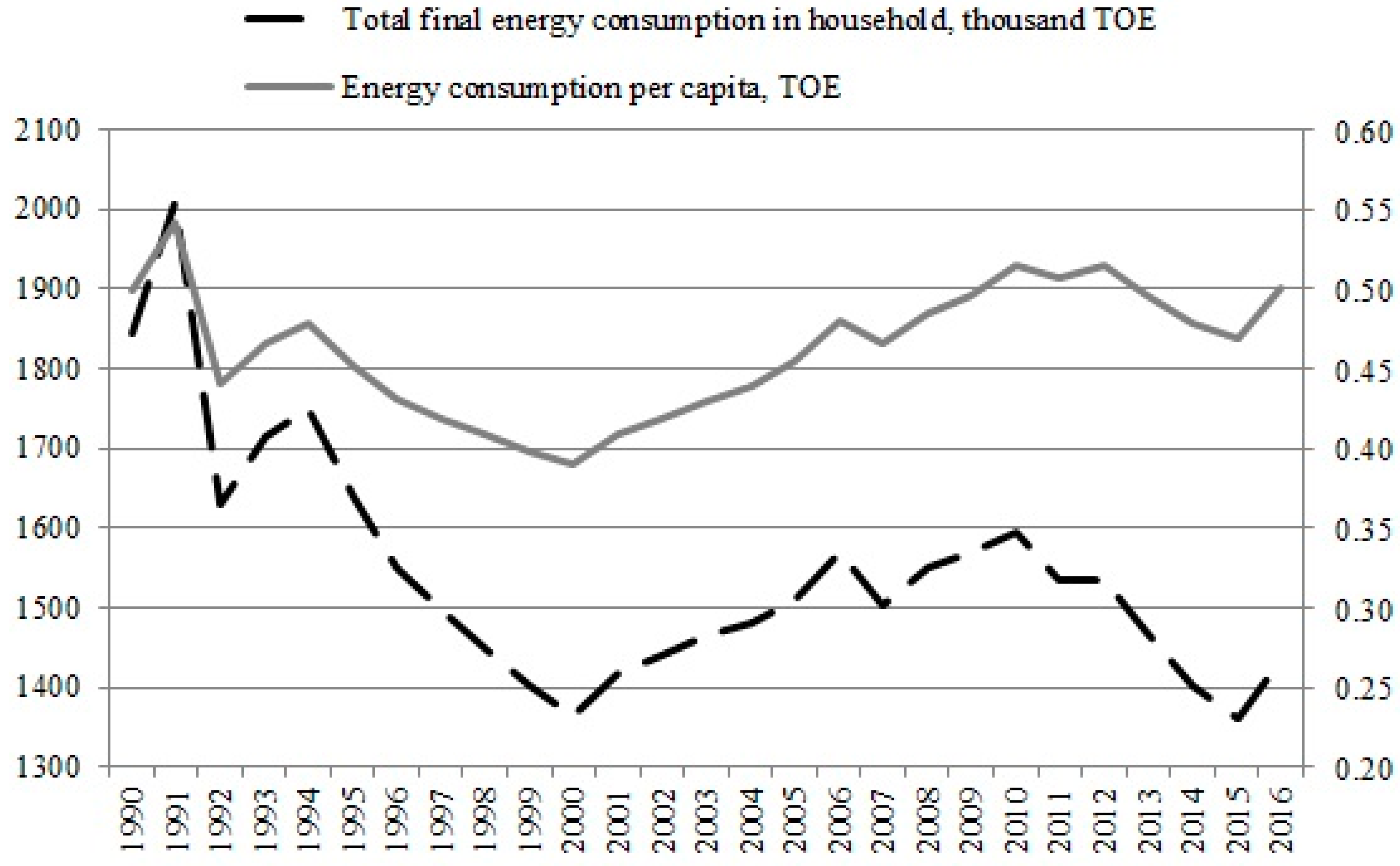
Residential energy consumption was decreasing for several years and reached the lowest level in 2015 (see Figure 1). Nevertheless, it rose in 2016 again. During that time, Lithuanian population decreased and this fact should be taken into account. The figures of energy consumption per capita reveal the real trends of energy consumption in the country. The calculations show that the level of energy consumption has decreased from 2010 but rose during 2016.
The rates of energy consumption in Lithuania are not high in comparison to the other EU Member States. In 2015, energy consumption per capita in Lithuania was 13.1% lower than the average energy consumption per capita in 28 EU Member States (see Figure 2).
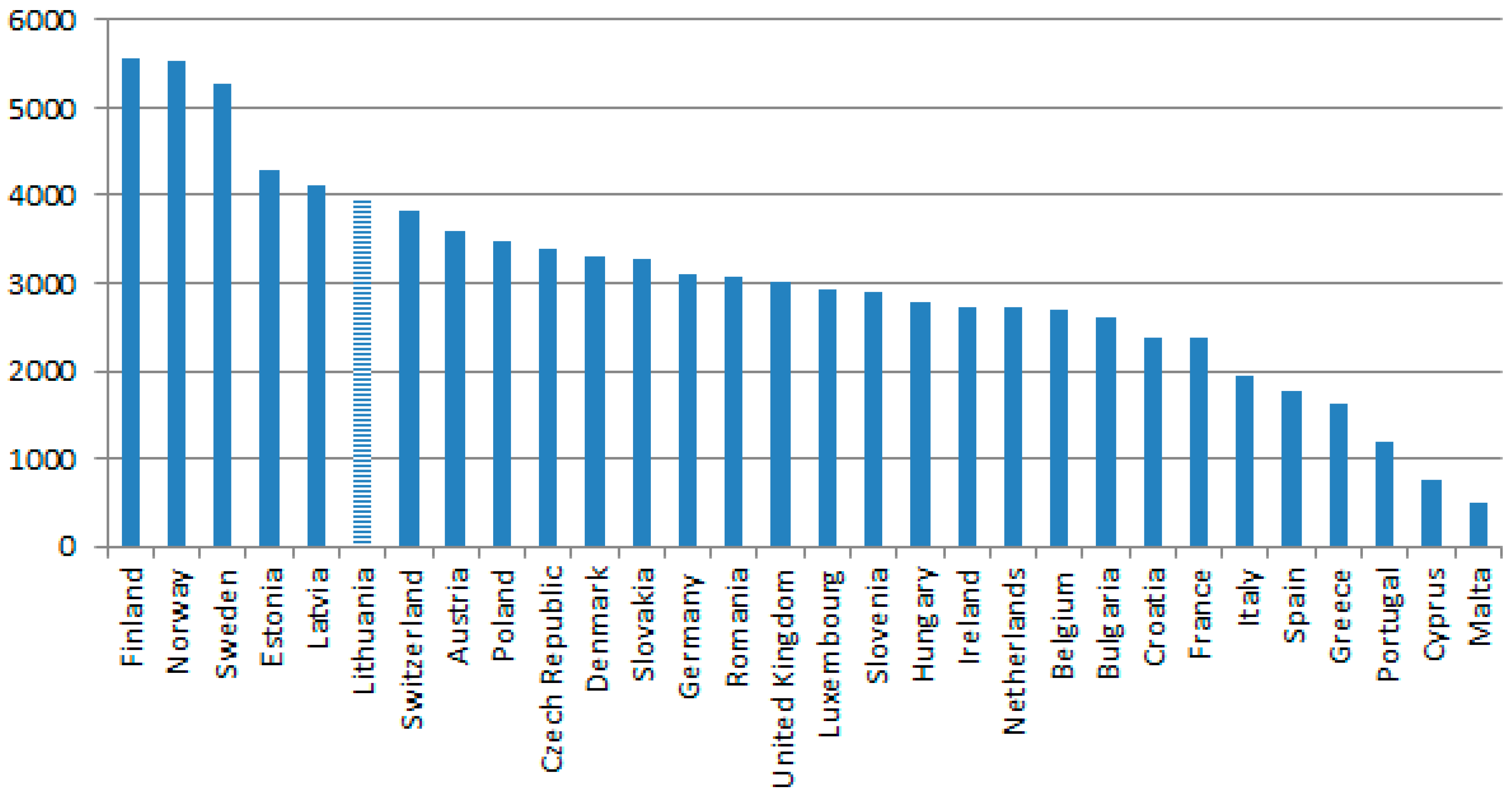
Lithuania’s geographic location should be taken into account in order to analyze the statistical data. Most of the states that consume less energy are located to the south of Lithuania. Therefore, the needs of these EU states for heating are considerably lower. Only Latvia, Estonia, Sweden, Norway and Finland have more heating days than Lithuania (see Figure 3). It means that residents from the states that are Luxembourg, Belgium, Denmark, Austria, Germany, France, the United Kingdom, the Netherlands, Ireland, Slovenia, Czech Republic, Hungary, Croatia, France, Italy and Poland (located to the left of Lithuania in Figure 2) consume less energy than Lithuanian residents.
Lithuanian residents spend really much on household energy bills. The average consumption expenditure per household member amounted to 297.5 euro per month in 2016 and it increased by 48% over ten years. Meanwhile, the expenditure for housing, water, electricity, gas and other fuels increased by 86% during the same period and amounted to 42.3 euro per month in 2016. The expenditure was twice higher in the largest cities as in rural areas. This type of expenditure accounted for 14.2% of all consumption expenditure per household member in 2016, while it accounted for about 11.4% in 2006.
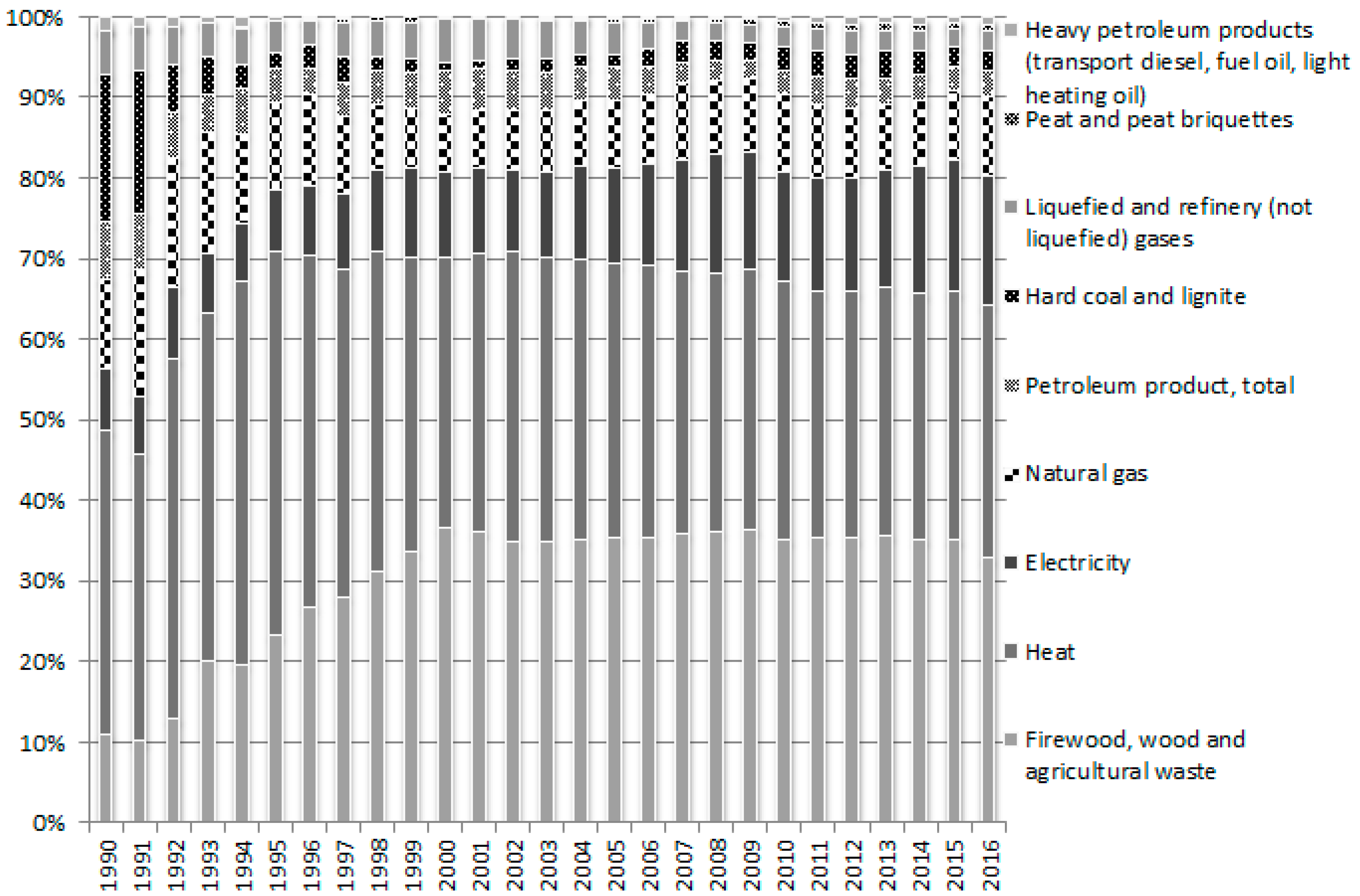
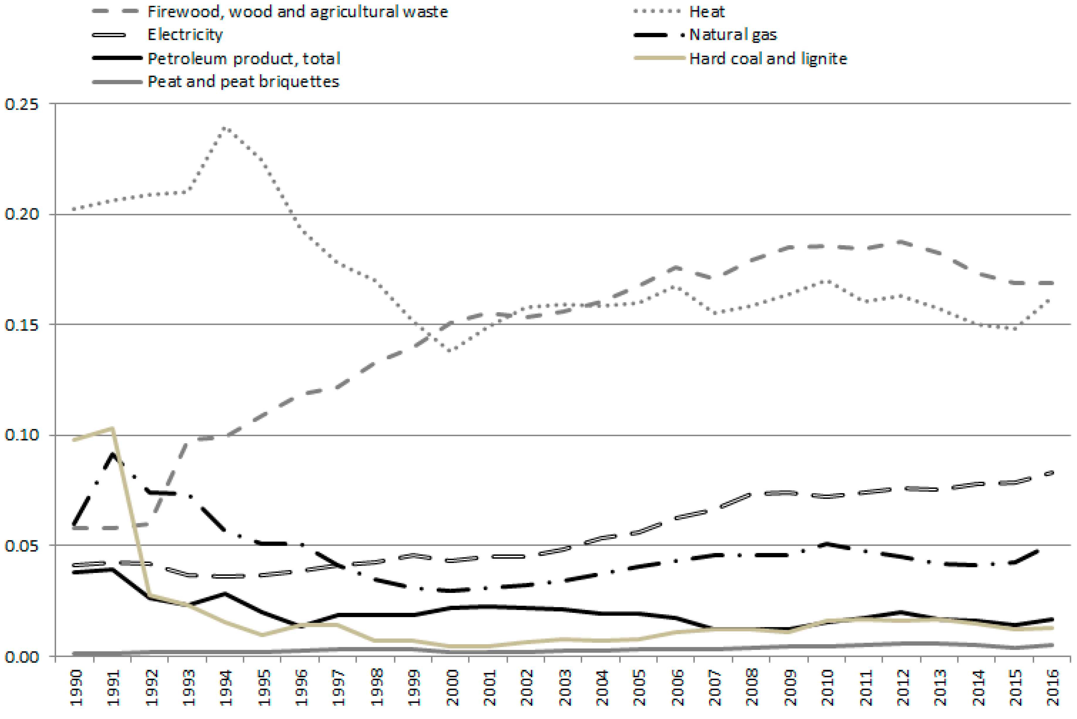
Figure 4 shows the structure of energy consumption per capita in Lithuania. Firewood, wood and agricultural waste, heat and electricity as the main energy commodities accounted for 83% of all the energy consumed in 2016 (firewood, wood and agricultural waste—33.8%, heat—32.5% and electricity—16.7%). Natural gas accounted for 10.1%, petroleum products—for 3.4%, hard coal and lignite—for 2.5% of all the energy consumed.
Consumption of the biggest part of energy commodities with the exception of firewood, wood and agricultural waste has decreased in Lithuania in recent years. The consumption of firewood, wood and agricultural waste increased by 42.4% over the last 20 years. However, the share of the above-mentioned fuels in the total amount of energy consumption has been decreasing for the last two years. Meanwhile, the share of electricity is constantly rising and the volume of electricity consumption increased more than twice over the last 20 years (see Figure 5). That is one of the reasons why household electricity consumption requires more scientific attention.
3.2. Electricity Consumption in Lithuania
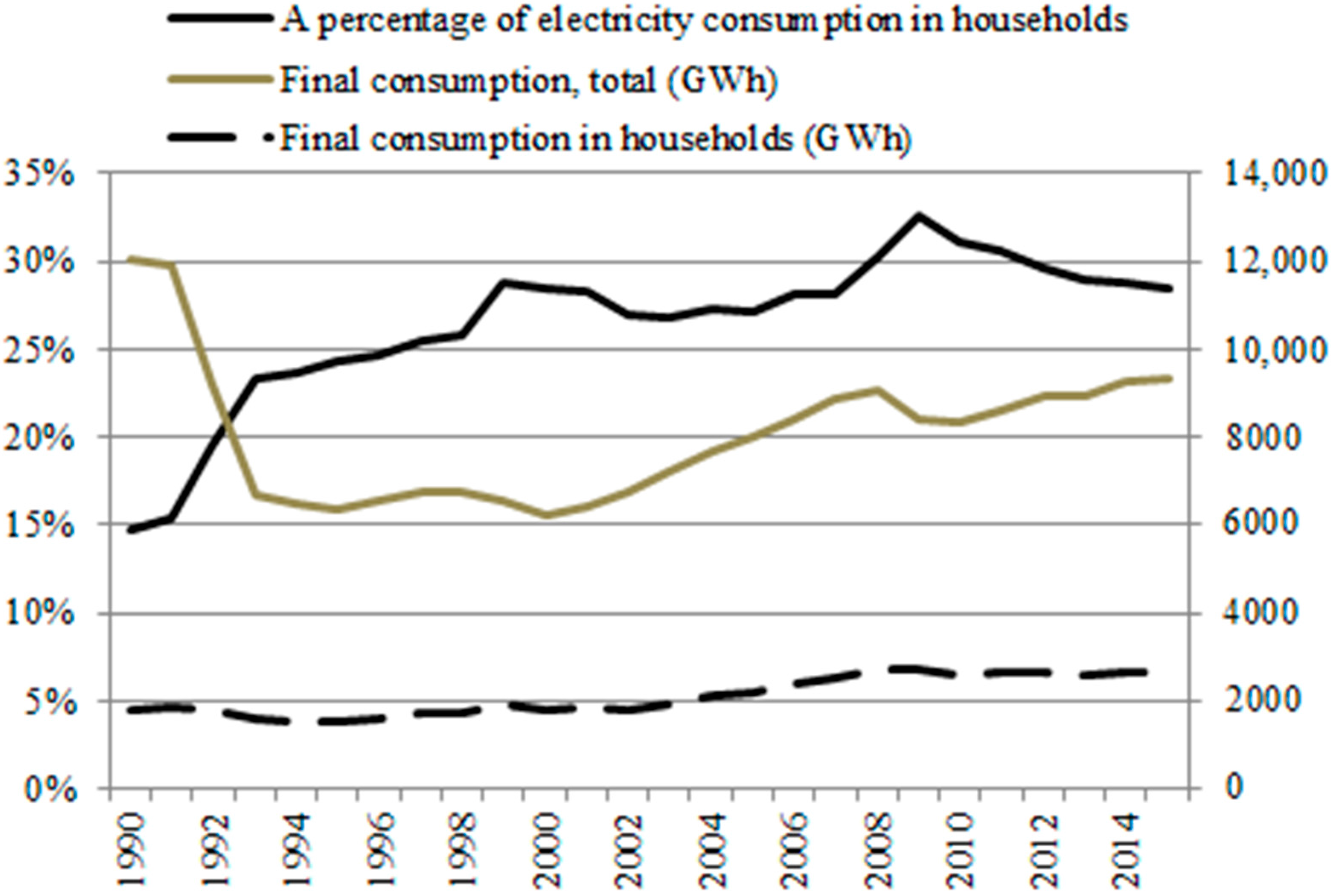
Total final consumption of electricity (consumed by households, industry, transport and other sectors) increased by 47% during the last 20 years, while the final consumption of electricity in households climbed 72.3% during the same period (see Figure 6). Therefore, the percentage of household electricity consumption has increased almost twice in the base of all final consumption of electricity in the country from 1990. Nevertheless, it has been moving downwards since 2010.
Even the increase of electricity price did not stop the rise of consumption. The price of electricity grew by nearly 50% (taking into account all the taxes) in Lithuania from 2004 to 2016. The price of electricity price has decreased recently, so that may have a negative impact on the efforts to reduce the volume of electricity consumption.
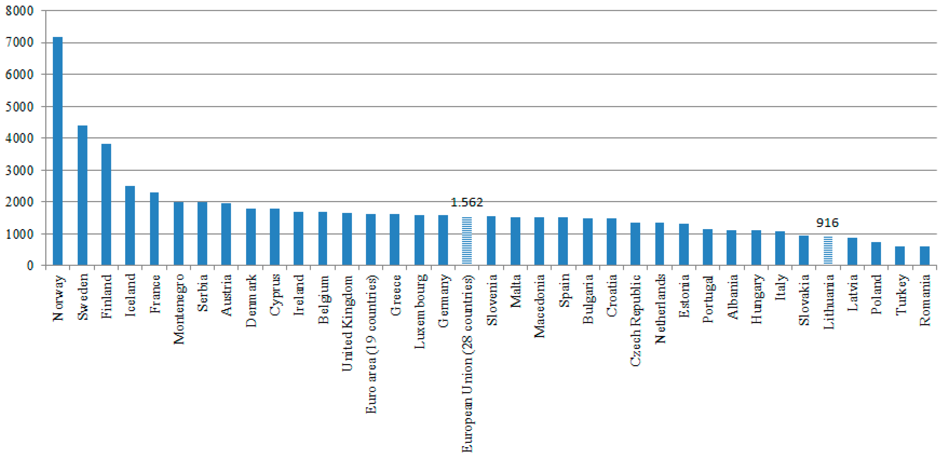
Nevertheless, electricity consumption per capita is not high in Lithuania by comparison to the other European countries (see Figure 7). So, Lithuania is on the right track. Lithuania outperformed Slovakia in 2014. At present only the households of Poland, Turkey, Latvia and Romania consume less electricity than Lithuanians. In general, electricity consumption is 41.4% lower than the EU-28 average in Lithuania.
The results of the survey of Lithuanian residents about their electricity consumption habits (conducted by the research company UAB Baltijos tyrimai, ordered by the electricity company ESO, AB) showed that 75% of the respondents save electricity [53]. 45% of the respondents do that due to high electricity prices and 47% of the respondents admit saving electricity because of their bad financial situation and low income.
Therefore, we can raise the question: is the rate of electricity consumption in Lithuania low because of the residents’ awareness to save energy or as low income of Lithuanian households? When answering this question, it is important to examine the relationship between the indicators of Lithuanian household electricity consumption and the social and economic indicators of the country.
3.3. The Impact of Economic and Social Factors on Household Electricity Consumption
Unit root test showed that only basic monthly wage, basic social benefit and heating degree days are stationary processes (i.e., all of them are stationary processes with intercept). While gross monthly average earnings, net monthly average earnings, average disposable income per month per household (in cash and in cash and kind), average disposable income per month in cash and kind per capita, average disposable income per month in cash per capita, at-risk-of-poverty threshold (both types of households), mean and median equivalised net income are the second-order integrated processes. All other indicators become stationary after the first-order differentiation without any trend or intercept (see Table 1).
Cointegration is tested for the first order integrated processes. The aim is to select the indicators that are cointegrated with residential electricity consumption per capita (log values of all indicators are analyzed). Engle-Granger cointegration test is used. Maximum lag order 3 is analyzed. The calculations reveal that five indicators, i.e., ratio of the registered unemployed to the working-age population, a heavy burden of housing expenses on households, at-risk-of-poverty rate, GDP at current prices and housing cost overburden rate are cointegrated with residential electricity consumption per capita at the 0.05 significance level (see Table 2).
Granger causality test is conducted as an additional test. If two or more time-series are cointegrated, then there must be Granger causality between them but in this case a conflict in the results exists. Although data are cointegrated, any evidence of causality between residential electricity consumption per capita and at-risk-of-poverty rate as well as housing cost overburden rate is not found (see Table 3). This might occur if the sample size is too small to satisfy the asymptotics that the cointegration and causality tests rely on (at-risk-of-poverty rate and housing cost overburden rate consist of only 12 observations). As a result, these two indicators are eliminated from the further analysis. Meanwhile there is strong evidence that ratio of the registered unemployed to the working-age population, a heavy burden of housing expenses on households and GDP at current prices Granger-cause electricity consumption per capita.
ARDL model is formulated using log values of the variables that are denoted as follows: y is log value of electricity consumption per capita, x1 is log value of GDP at current prices, x2 is ratio of the registered unemployed to the working-age population and x3 is log value of a heavy burden of housing expenses on households. Maximum lags are determined by using BIC and it is 1 for all variables. The results are presented in Table 4.
The results are not satisfactory as the model is not significant and residuals are autocorrelated. Short time series of a heavy burden of housing expenses on households (12 observations) restricts to correct the model. As a consequence, this indicator is eliminated from the further analysis and unrestricted ECM is re-estimated with two explanatory variables. Although the precision of the model significantly decreased, the model is significant and residuals are not autocorrelated (see Table 5).
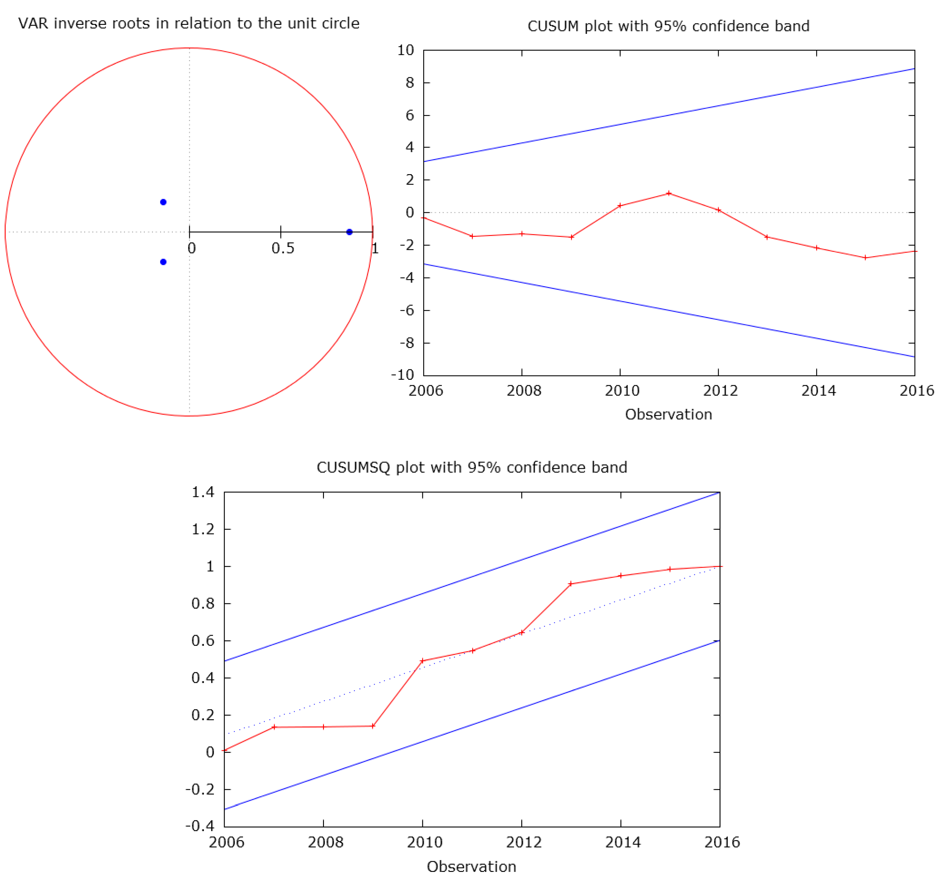
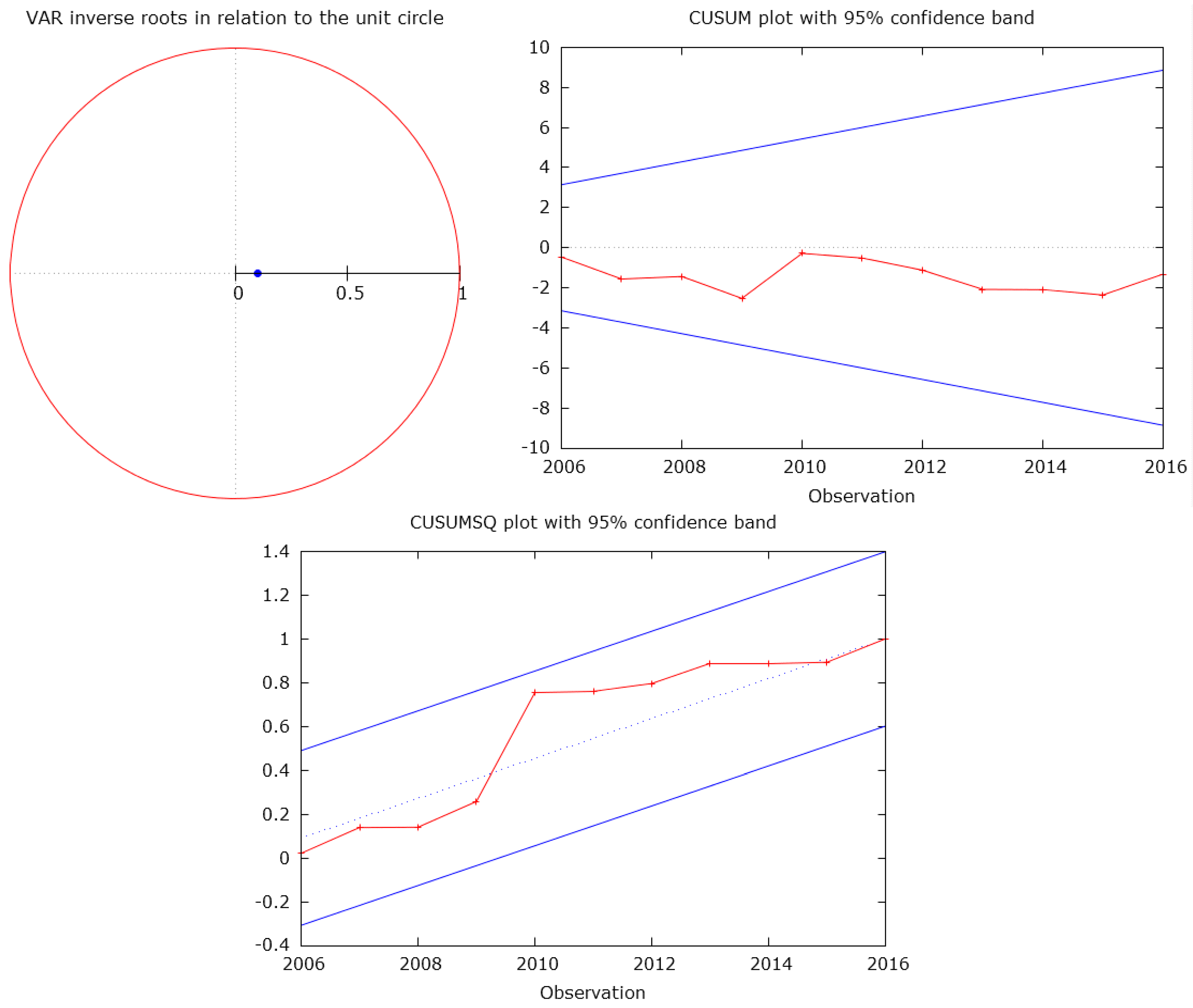
The model is dynamically stable as the inverse roots are all inside the unit circle (Figure 8). In order to ensure the stability of the long-run parameters, the CUSUM and the CUSUMQ tests are also applied. In both graphs (see Figure 8), the blue lines represent the critical upper and lower bounds at the 5% level of significance. The visual inspection of graphs reveals that there is no evidence of parameters instability, since the cumulated sum of scaled residuals and the cumulated sum of the squared residuals move within the critical bounds.
Wald test on VAR is performed to test the null hypothesis that the regression parameters are zero for the variables yt−1, x1 t−1 and x2 t−1. The calculations reveal that χ2 = 21.0315 and p-value is 0.0125. The results confirm the existence of a long-run relationship.
As the bounds test leads to the conclusion of cointegration, the long-run equilibrium relationship between the variables can be estimated. Results presented in Table 5 indicate that the long-run multiplier between electricity consumption per capita and GDP at current prices is 0.5346, meanwhile long-run multiplier between electricity consumption per capita and ratio of the registered unemployed to the working-age population is −0.2284. It means that in the long run, an increase of 1% in GDP at current prices will lead to an increase of 0.5346% in electricity consumption per capita, while increase of 1% in ratio of the registered unemployed to the working-age population will lead to a decrease of 0.2284% in electricity consumption per capita.
OLS estimates of Equation (5) are presented in Table 6. Although model is significant and precision of the model quite high, the parameter of the ratio of the registered unemployed to the working-age population is not significant. Residuals of the model are distributed by normal distribution (χ2(2) = 4.629 and p-value is 0.0988) and they are not autocorrelated.
The final step is the estimation of the short-run dynamic coefficients via the usual error correction model. Estimates of usual ECM are presented in Table 7. The coefficient of the error-correction term, zt−1, is negative but not significant. Its value indicates that deviations from equilibrium are restored to an annual rate of approximately 74%.
Residuals of the model are distributed by normal distribution (χ2(2) = 0.007 and p-value is 0.9964) and they are not autocorrelated. The model is also dynamically stable as the inverse roots are all inside the unit circle. The CUSUM and the CUSUMQ graphs confirm that there is no evidence of parameters instability, since the cumulated sum of scaled residuals and the cumulated sum of the squared residuals move within the critical bounds (see Figure 9).
4. Discussion
The research has revealed that social and economic situation in Lithuania has a significant impact on residential electricity consumption. This study leads to conclude that there is a long run equilibrium relationship between electricity consumption per capita and GDP at current prices as well as the ratio of the registered unemployed to the working-age population. In other words, these indicators are not drifting farther from each other in the long run. In the long run, an increase of 1% in GDP at current prices will lead to an increase of 0.5346% in electricity consumption per capita, while increase of 1% in ratio of the registered unemployed to the working-age population will lead to a decrease of 0.2284% in electricity consumption per capita.
A heavy burden of housing expenses on households is also found to be cointegrated with residential electricity consumption per capita but statistically significant evaluation of its impact is problematic because of short time series. The impact of at-risk-of-poverty rate and housing cost overburden rate on electricity consumption per capita is also under discussion and its evaluation is problematic for the same reason. As a consequence, this study should be repeated after some years to clarify the results.
Though residential electricity consumption depends on financial situation of the households, the potential to reduce the use of electricity is comparatively low. Housing expenses are significant for about 90% of Lithuanian households. That means that this share of population is already characterized by electricity saving. This leads to the conclusion that electricity consumption in Lithuania is low due to the poor financial situation of Lithuanian households but not due to their awareness to save energy. The improvement of economic and social situation in the country as well as the growth of welfare in communities is the main task of Lithuanian government. In turn, higher living standards should promote Lithuanian people to pay particular attention to sustainable electricity consumption on condition that they are provided with the appropriate information and feedback on how to keep energy consumption low. The results of this research can contribute to promotion of electricity saving aligned with the changes in economic and social situation in Lithuania. It also may help to evaluate the actual benefit of the measures that are employed for promotion of sustainable electricity consumption in Lithuanian households.
Author Contributions
Sergej Vojtovic contributed to the design of the article title, provided advice on results and modified the manuscript. Alina Stundziene reviewed the literature, carried out analysis and wrote the majority of the manuscript. Rima Kontautiene joined the literature review and discussion and contributed to writing the paper. All authors have read and approved the final manuscript.
Conflicts of Interest
The authors declare no conflicts of interest.
References
- Ates, S.A.; Durakbasa, N.M. Evaluation of corporate energy management practices of energy intensive industries in Turkey. Energy 2012, 45, 81–91. [Google Scholar] [CrossRef]
- Kahraman, C.; Kaya, I. A fuzzy multi-criteria methodology for selection among energy alternatives. Expert Syst. Appl. 2010, 37, 6270–6281. [Google Scholar] [CrossRef]
- Zolfani, S.H.; Saparauskas, J. New application of SWARA method in prioritizing sustainability assessment indicators of energy system. Eng. Econ. 2013, 24, 408–414. [Google Scholar] [CrossRef]
- Klevas, V.; Streimikiene, D.; Grikstaite, R. Sustainable energy in Baltic States. Energy Policy 2007, 35, 76–90. [Google Scholar] [CrossRef]
- Bilgen, S.; Keles, S.; Kaygusuz, A.; Sari, A.; Kaygusuz, K. Global warming and renewable energy sources for sustainable development: A case study in Turkey. Renew. Sustain. Energy Rev. 2008, 12, 372–396. [Google Scholar] [CrossRef]
- Omer, A.M. Energy, environment and sustainable development. Renew. Sustain. Energy Rev. 2008, 12, 2265–2300. [Google Scholar] [CrossRef]
- Yuksel, I. Hydropower in Turkey for a clean and sustainable energy future. Renew. Sustain. Energy Rev. 2008, 12, 1622–1640. [Google Scholar] [CrossRef]
- Directive 2012/27/EU of the European Parliament and of the Council of 25 October 2012 on Energy Efficiency, Amending Directives 2009/125/EC and 2010/30/EU and Repealing Directives 2004/8/EC and 2006/32/EC. Available online: http://eur-lex.europa.eu/legal-content/EN/TXT/?uri=celex%3A32012L0027 (accessed on 20 November 2017).
- Dahlquist, E.; Vassileva, I.; Thorin, E.; Wallin, F. How to save energy to reach a balance between production and consumption of heat, electricity and fuels for vehicles. Energy 2012, 46, 16–20. [Google Scholar] [CrossRef]
- Filippini, M.; Hunt, L.C.; Zoric, J. Impact of energy policy instruments on the estimated level of underlying energy efficiency in the EU residential sector. Energy Policy 2014, 69, 73–81. [Google Scholar] [CrossRef]
- Yohanis, Y.G.; Mondol, J.D.; Wright, A.; Norton, B. Real-life energy use in the UK: How occupancy and dwelling characteristics affect domestic electricity use. Energy Build. 2008, 40, 1053–1059. [Google Scholar] [CrossRef]
- Communication from the Commission to the European Parliament, the Council, the European Economic and Social Committee and the Committee of the Regions. Energy 2020—A Strategy for Competitive, Sustainable and Secure Energy. COM (2010) 639 Final, Brussels. 10 November 2010. Available online: http://eur-lex.europa.eu/legal-content/EN/TXT/?uri=celex:52010DC0639 (accessed on 20 November 2017).
- Chontanawat, J.; Hunt, L.C.; Pierse, R. Does energy consumption cause economic growth? Evidence from a systematic study of over 100 countries. J. Policy Model. 2008, 30, 209–220. [Google Scholar] [CrossRef]
- Lee, C. Energy consumption and GDP in developing countries: A cointegrated panel analysis. Energy Econ. 2005, 27, 415–427. [Google Scholar] [CrossRef]
- Soytas, U.; Sari, R. Energy consumption and GDP: Causality relationship in G-7 countries and emerging markets. Energy Econ. 2003, 25, 33–37. [Google Scholar] [CrossRef]
- Filippini, M.; Hunt, L.C. US residential energy demand and energy efficiency: A stochastic demand frontier approach. Energy Econ. 2012, 34, 1484–1491. [Google Scholar] [CrossRef]
- Filippini, M.; Hunt, L.C. Underlying Energy Efficiency in the US; School of Economics, University of Surrey: Guildford, UK, 2015; Available online: http://www.seec.surrey.ac.uk/research/SEEDS/SEEDS150.pdf (accessed on 12 October 2017).
- Schlor, H.; Fischer, W.; Hake, J.F. Methods of measuring sustainable development of the German energy sector. Appl. Energy 2013, 101, 172–181. [Google Scholar] [CrossRef]
- Lior, N. Sustainable energy development with some game-changers. Energy 2012, 40, 3–18. [Google Scholar] [CrossRef]
- Asafu-Adjaye, J. The relationship between energy consumption, energy prices and economic growth: Time series evidence from Asian developing countries. Energy Econ. 2000, 22, 615–625. [Google Scholar] [CrossRef]
- Daioglou, V.; Faaij, A.P.C.; Saygin, D.; Patel, M.K.; Wicke, B.; van Vuuren, D.P. Energy demand and emissions of the non-energy sector. Energy Environ. Sci. 2014, 7, 482–498. [Google Scholar] [CrossRef]
- Phdungsilp, A. Projections of energy use and carbon emissions for Bangkok, Thailand. J. Rev. Glob. Econ. 2017, 6, 248–257. [Google Scholar] [CrossRef]
- Phdungsilp, A.; Wuttipornpun, T. Energy and carbon modeling with multi-criteria decision-making towards sustainable industrial sector development in Thailand. Low Carbon Econ. 2011, 2, 165–172. [Google Scholar] [CrossRef]
- Saygin, D.; Worrell, E.; Patel, M.K.; Gielen, D.J. Benchmarking the energy use of energy-intensive industries in industrialized and in developing countries. Energy 2011, 36, 6661–6673. [Google Scholar] [CrossRef]
- Saygin, D.; Worrell, E.; Tam, C.; Trudeau, N.; Gielen, D.J.; Weiss, M.; Patel, M.K. Long-term energy efficiency analysis requires solid energy statistics: The case of the German basic chemical industry. Energy 2012, 44, 1094–1106. [Google Scholar] [CrossRef]
- Siitonen, S.; Tuomaala, M.; Ahtila, P. Variables affecting energy efficiency and CO2 emissions in the steel industry. Energy Policy 2010, 38, 2477–2485. [Google Scholar] [CrossRef]
- Brosch, T.; Patel, M.K.; Sander, D. Affective influences on energy-related decisions and behaviors. Front. Energy Res. 2014, 2, 1–12. [Google Scholar] [CrossRef]
- Srovnalikova, P.; Karbach, R. Tax Changes and Their Impact on Managerial Decision Making. In Proceedings of the 1st International Conference Contemporary Issues in Theory and Practice of Management (CITPM 2016), Czestochowa, Poland, 21–22 April 2016; Okreglicka, M., Gorzen-Mitka, I., Lemanska-Majdzik, A., Sipa, M., Skibinski, A., Eds.; Wydawnictwo Wydzialu Zarzadzania Politechniki Czestochowskiej: Czestochowa, Poland, 2016; pp. 410–415, ISBN 978-83-65179-43-2. [Google Scholar]
- Filippini, M.; Hunt, L.C. Energy demand and energy efficiency in the OECD countries: A stochastic demand frontier approach. Energy J. 2011, 32, 59–80. [Google Scholar] [CrossRef]
- Evans, J.; Filippini, M.; Hunt, L.C. Measuring Energy Efficiency and Its Contribution towards Meeting CO2 Targets: Estimates for 29 OECD Countries; School of Economics, Discussion Papers (SEEDS) 135; School of Economics, University of Surrey: Guildford, UK, 2011; pp. 1–36. Available online: http://www.seec.surrey.ac.uk/research/SEEDS/SEEDS135.pdf (accessed on 12 October 2017).
- Vassileva, I.; Campillo, J. Increasing energy efficiency in low-income households through targeting awareness and behavioral change. Renew. Energy 2014, 67, 59–63. [Google Scholar] [CrossRef]
- Martinsson, J.; Lundqvist, L.J.; Sundstrom, A. Energy saving in Swedish households. The (relative) importance of environmental attitudes. Energy Policy 2011, 39, 5182–5191. [Google Scholar] [CrossRef]
- Rakauskiene, O.G.; Strunz, H. Approach to reduction of socioeconomic inequality: Decrease of vulnerability and strengthening resilience. Econ. Sociol. 2016, 9, 243–258. [Google Scholar] [CrossRef]
- Vassileva, I.; Campillo, J.; Wallin, F.; Dahlquist, E. Comparing the characteristics of different high-income households in order to improve energy awareness strategies. In Proceedings of the 5th International Conference on Appl. Energy (ICAE 2013), Pretoria, South Africa, 1–4 July 2013; Available online: https://www.researchgate.net/publication/254864543_Comparing_the_characteristics_of_different_high-income_households_in_order_to_improve_energy_awareness_strategies (accessed on 12 October 2017).
- Vassileva, I.; Dahlquist, E.; Wallin, F.; Campillo, J. Energy consumption feedback devices’ impact evaluation on domestic energy use. Appl. Energy 2013, 106, 314–320. [Google Scholar] [CrossRef]
- Bertholet, J.L.; Cabrera, S.J.D.; Lachal, B.M.; Patel, M.K. Evaluation of an energy efficiency program for small customers in Geneva. In Proceedings of the IEPEC International Energy Program Evaluation Conference, Berlin, Germany, 9–11 September 2014; Available online: https://archive-ouverte.unige.ch/unige:41571 (accessed on 12 October 2017).
- Dilaver, Z.; Hunt, L.C. Industrial electricity demand for Turkey: A structural time series analysis. Energy Econ. 2011, 33, 426–436. [Google Scholar] [CrossRef] [Green Version]
- McLoughlin, F.; Duffy, A.; Conlon, M. Characterising domestic electricity consumption patterns by dwelling and occupant socio-economic variables: An Irish case study. Energy Build. 2012, 48, 240–248. [Google Scholar] [CrossRef]
- Lin, W.; Chen, B.; Luo, S.; Liang, L. Factor analysis of residential energy consumption at the provincial level in China. Sustainability 2014, 6, 7710–7724. [Google Scholar] [CrossRef]
- Ding, Y.; Qu, W.; Niu, S.; Liang, M.; Qiang, W.; Hong, Z. Factors influencing the spatial difference in household energy consumption in China. Sustainability 2016, 8, 1285. [Google Scholar] [CrossRef]
- Zhao, C.S.; Ni, S.-W.; Zhang, X. Effects of household energy consumption on environment and its influence factors in rural and urban areas. Energy Procedia 2012, 14, 805–811. [Google Scholar] [CrossRef]
- Santin, O.G.; Itard, L.; Visscher, H. The effect of occupancy and building characteristics on energy use for space and water heating in Dutch residential stock. Energy Build. 2009, 41, 1223–1232. [Google Scholar] [CrossRef]
- Supasa, T.; Hsiau, S.S.; Lin, S.M.; Wongsapai, W.; Wu, J.C. Household energy consumption behaviour for different demographic regions in Thailand from 2000 to 2010. Sustainability 2017, 9, 2328. [Google Scholar] [CrossRef]
- Dergiades, T.; Tsoulfidis, L. Estimating residential demand for electricity in the United States, 1965–2006. Energy Econ. 2008, 30, 2722–2730. [Google Scholar] [CrossRef]
- Pachauri, S.; Jiang, L. The household energy transition in India and China. Energy Policy 2008, 36, 4022–4035. [Google Scholar] [CrossRef]
- Fuller, R.J.; Crawford, R.H. Impact of past and future residential housing development patterns on energy demand and related emissions. J. Hous. Built Envrion. 2011, 26, 165–183. [Google Scholar] [CrossRef]
- Stephan, A.; Crawford, R.H.; Myttenaere, K. Multi-scale life cycle energy analysis of a low-density suburban neighbourhood in Melbourne, Australia. Build. Envrion. 2013, 68, 35–49. [Google Scholar] [CrossRef]
- VandeWeghe, J.R.; Kennedy, C. A spatial analysis of residential greenhouse gas emissions in the Toronto census metropolitan area. J. Ind. Ecol. 2007, 11, 133–144. [Google Scholar] [CrossRef]
- Heinonen, J.; Junnila, S. Residential energy consumption patterns and the overall housing energy requirements of urban and rural households in Finland. Energy Build. 2014, 76, 295–303. [Google Scholar] [CrossRef]
- Dergiades, T.; Tsoulfidis, L. Revisiting residential demand for electricity in Greece: New evidence from the ARDL approach to cointegration analysis. Empir. Econ. 2011, 41, 511–531. [Google Scholar] [CrossRef]
- Vassileva, I.; Wallin, F.; Dahlquist, E. Understanding energy consumption behavior for future demand response strategy development. Energy 2012, 46, 94–100. [Google Scholar] [CrossRef]
- Krajnakova, E.; Navikaite, A.; Navickas, V. Paradigm shift of small and medium-sized enterprises competitive advantage to management of customer satisfaction. Eng. Econ. 2015, 26, 327–332. [Google Scholar] [CrossRef]
- ESO. Tyrimas: Gyventojai Elektrą Taupo Iš Įpročio ir Tausodami Aplinką. 2015. Available online: http://www.eso.lt/lt/ziniasklaida/p50/tyrimas-gyventojai-elektra-taupo-is-iprocio-ir-3fuz.html (accessed on 10 October 2016).
Figure 1.
The energy consumption per capita (in tonnes of oil equivalent—TOE) and total final energy consumption (in thousand TOE) in Lithuania.
Figure 1.
The energy consumption per capita (in tonnes of oil equivalent—TOE) and total final energy consumption (in thousand TOE) in Lithuania.

Figure 2.
Energy consumption per capita in 2015 (in TOE).
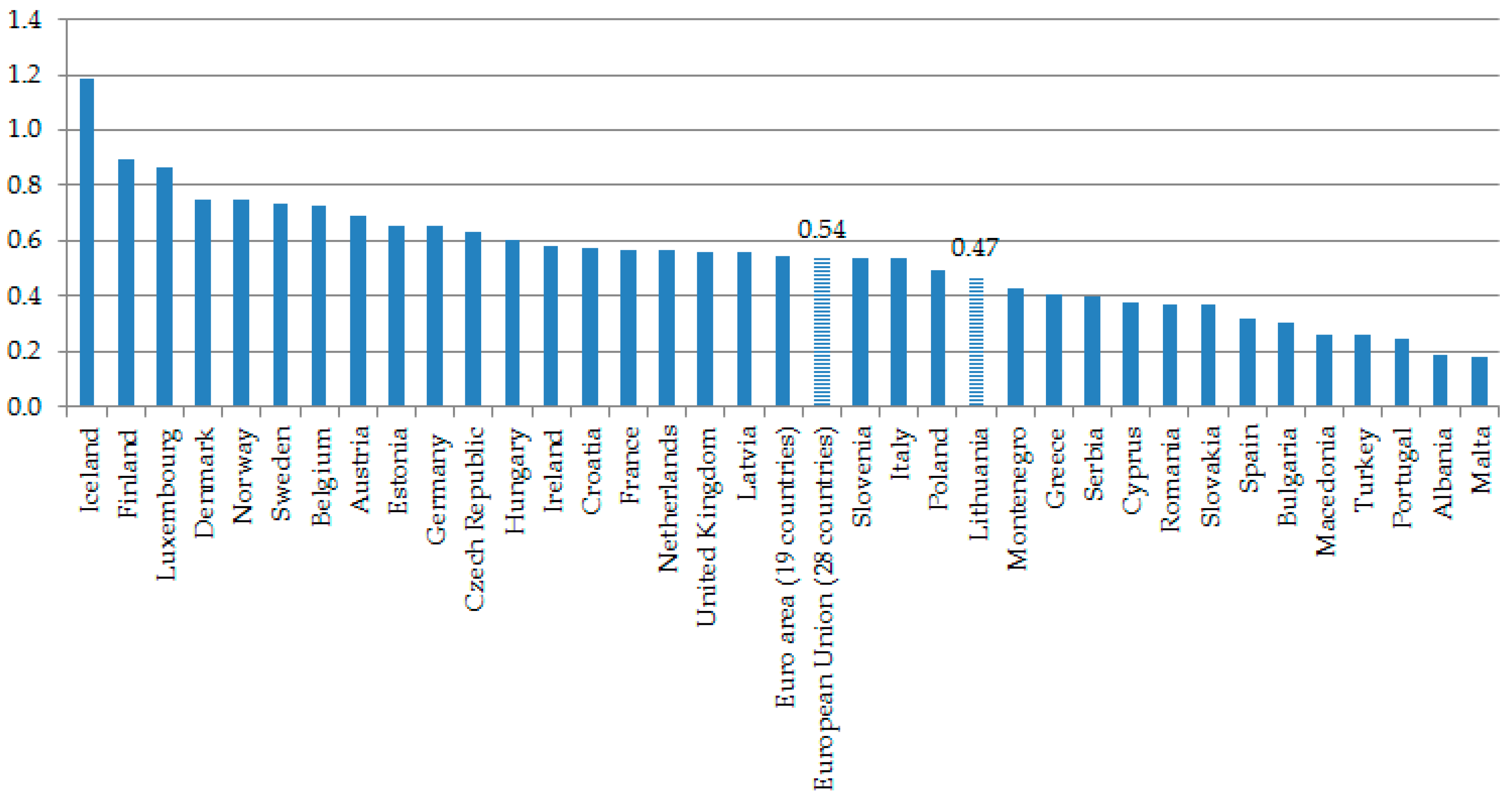
Figure 3.
Actual heating degree-days (the average of 1995–2016).

Figure 4.
Structure of energy consumption per capita.

Figure 5.
The tendency of energy consumption (in TOE) per capita during 1990–2016.

Figure 6.
Final consumption of electricity in Lithuania.

Figure 7.
Electricity consumption (KWh) per capita in 2015.

Figure 8.
Inverse roots and CUSUM and CUSUMSQ plots with 95% confidence band.

Figure 9.
Inverse roots and CUSUM and CUSUMSQ plots with 95% confidence band.


Table 1.
ADF unit root test.
| Social or Economic Indicator | Integration |
|---|---|
| Residential electricity consumption per capita | I(1) without constant |
| Stock of dwellings | I(1) without constant |
| Useful floor area per capita | I(1) without constant |
| Electricity prices for domestic consumers with taxes and levies | I(1) without constant |
| Electricity prices before taxes and levies | I(1) without constant |
| Heating degree days | I(0) with constant |
| Unemployment | I(1) without constant |
| Ratio of the registered unemployed to the working-age population | I(1) without constant |
| Gross monthly average earnings | I(2) |
| Net monthly average earnings | I(2) |
| Basic monthly wage | I(0) with constant |
| Basic social benefit | I(0) with constant |
| Average disposable income per month in cash and kind per household | I(2) |
| Average disposable income per month in cash and kind per capita | I(2) |
| Average disposable income per month in cash per household | I(2) |
| Average disposable income per month in cash per capita | I(2) |
| A heavy burden of housing expenses on households | I(1) without constant |
| A slight burden of housing expenses on households | I(1) without constant |
| Not burden of housing expenses on households at all | I(1) without constant |
| At-risk-of-poverty threshold, type of household: single person | I(2) |
| At-risk-of-poverty threshold, type of household: 2 adults with 2 children younger than 14 years | I(2) |
| At-risk-of-poverty gap | I(1) without constant |
| At-risk-of-poverty rate | I(1) without constant |
| GDP at current prices | I(1) without constant |
| GDP per capita at current prices | I(1) without constant |
| Mean equivalised net income | I(2) |
| Median equivalised net income | I(2) |
| Overcrowding rate | I(1) without constant |
| Housing cost overburden rate | I(1) without constant |
Table 2.
Augmented Dickey-Fuller test (p-values) for the residuals from the cointegrating regression.
Table 2.
Augmented Dickey-Fuller test (p-values) for the residuals from the cointegrating regression.
| Social or Economic Indicator | Cointegrating Regression | ||
|---|---|---|---|
| Without Constant | With Constant | With Constant and Trend | |
| Stock of dwellings | 0.8344 | 0.7644 | 0.08844 * |
| Useful floor area per capita | 0.2499 | 0.8042 | 0.1281 |
| Electricity prices for domestic consumers with taxes and levies | 0.6416 | 0.1102 | 0.8356 |
| Electricity prices before taxes and levies | 0.39 | 0.09263 * | 0.8415 |
| Unemployment | 0.1475 | 0.9456 | 0.4599 |
| Ratio of the registered unemployed to the working-age population | 0.01237 ** | 0.9243 | 0.5102 |
| A heavy burden of housing expenses on households | 0.01643 ** | 0.312 | 0.489 |
| A slight burden of housing expenses on households | 0.3778 | 0.7135 | 0.5206 |
| Not burden of housing expenses on households at all | 0.05084 * | 0.6264 | 0.4221 |
| At-risk-of-poverty gap | 0.09932 * | 0.5095 | 0.1202 |
| At-risk-of-poverty rate | 0.02983 ** | 0.7247 | 0.02881 ** |
| GDP at current prices | 0.006181 *** | 0.04325 ** | 0.2876 |
| GDP per capita at current prices | 0.1355 | 0.06163 * | 0.2336 |
| Overcrowding rate | 0.6122 | 0.2512 | 0.4341 |
| Housing cost overburden rate | 0.02673 ** | 0.2623 | 0.7254 |
***, ** and * denote significance at the 1, 5 and 10% significance level, respectively
Table 3.
The results of Granger causality test.
| Null Hypothesis | Max Lag of VAR | p-Value of Ljung-Box Test | Probability of H0 |
|---|---|---|---|
| H0: ratio of the registered unemployed to the working-age population does not Granger-cause y * | 2 | 0.555 | 0.0127 ** |
| H0: y does not Granger-cause ratio of the registered unemployed to the working-age population | 2 | 0.48 | 0.3526 |
| H0: a heavy burden of housing expenses on households does not Granger-cause y | 2 | 0.476 | 0.0105** |
| H0: y does not Granger-cause a heavy burden of housing expenses on households | 2 | 0.562 | 0.5689 |
| H0: at-risk-of-poverty rate does not Granger-cause y | 1 | 0.907 | 0.3249 |
| H0: y does not Granger-cause at-risk-of-poverty rate | 1 | 0.751 | 0.2446 |
| H0: GDP at current prices does not Granger-cause y | 1 | 0.263 | 0.0188 ** |
| H0: y does not Granger-cause GDP at current prices | 1 | 0.533 | 0.5037 |
| H0: housing cost overburden rate does not Granger-cause y | 2 | 0.844 | 0.9770 |
| H0: y does not Granger-cause housing cost overburden rate | 2 | 0.409 | 0.2643 |
* y denotes electricity consumption per capita; ** denote significance at the 5% significance level
Table 4.
Estimates of unrestricted ECM.
| Coefficient | Std. Error | t-Ratio | p-Value | |
|---|---|---|---|---|
| const | 5.95372 | 1.31267 | 4.536 | 0.1382 |
| −0.687914 | 0.285551 | −2.409 | 0.2505 | |
| −0.165628 | 0.07074 | −2.341 | 0.257 | |
| −0.141257 | 0.022921 | −6.163 | 0.1024 | |
| 0.099619 | 0.046063 | 2.163 | 0.2757 | |
| −0.652372 | 0.445884 | −1.463 | 0.3817 | |
| −0.0173455 | 0.179583 | −0.09659 | 0.9387 | |
| 0.057235 | 0.040701 | 1.406 | 0.3935 | |
| −0.398144 | 0.062584 | −6.362 | 0.0993 * | |
| Adjusted R-squared | 0.986680 | Schwarz criterion | −82.71503 | |
| F(8, 1) | 84.33608 | p-value (F) | 0.084030 |
* denote coefficient significance at the 10% significance level.
Table 5.
Estimates of unrestricted ECM with two explanatory variables.
| Coefficient | Std. Error | t-Ratio | p-Value | |
|---|---|---|---|---|
| const | 0.399903 | 0.28973 | 1.38 | 0.1949 |
| −0.502307 | 0.368351 | −1.364 | 0.1999 | |
| 0.134839 | 0.209446 | 0.6438 | 0.5329 | |
| −0.0379285 | 0.063739 | −0.5951 | 0.5638 | |
| −0.212269 | 0.40262 | −0.5272 | 0.6085 | |
| 0.113474 | 0.241696 | 0.4695 | 0.6479 | |
| −0.0484724 | 0.034821 | −1.392 | 0.1914 | |
| Adjusted R-squared | 0.460468 | Schwarz criterion | −59.63624 | |
| F(6, 11) | 3.418129 | p-value (F) | 0.037236 | |
| p-value of Ljung-Box test | l = 1 | l = 2 | l = 3 | l = 4 |
| 0.177 | 0.402 | 0.147 | 0.139 |
Table 6.
OLS estimates.
| Coefficient | Std. Error | t-Ratio | p-Value | |
|---|---|---|---|---|
| const | 0.623541 | 0.223251 | 2.793 | 0.0125 ** |
| 0.58513 | 0.022383 | 26.14 | 3.62 × 10⁻¹⁵ *** | |
| 0.02823 | 0.021073 | 1.34 | 0.198 | |
| Adjusted R-squared | 0.973696 | Schwarz criterion | −65.56116 | |
| F(2, 17) | 352.6668 | p-value(F) | 1.44 × 10⁻¹⁴ | |
| p-value of Ljung-Box test | l = 1 | l = 2 | l = 3 | l = 4 |
| 0.389 | 0.624 | 0.659 | 0.403 |
*** and ** denote coefficient significance at the 1 and 5% significance level, respectively.
Table 7.
Estimates of usual ECM.
| Coefficient | Std. Error | t-Ratio | p-Value | |
|---|---|---|---|---|
| const | −0.00656340 | 0.020176 | −0.3253 | 0.7511 |
| 0.098994 | 0.337717 | 0.2931 | 0.7749 | |
| 0.287886 | 0.242526 | 1.187 | 0.2602 | |
| 0.304718 | 0.201117 | 1.515 | 0.1579 | |
| 0.02472 | 0.077465 | 0.3191 | 0.7556 | |
| 0.056222 | 0.076746 | 0.7326 | 0.4791 | |
| −0.737742 | 0.414539 | −1.780 | 0.1027 | |
| Adjusted R-squared | 0.480183 | Schwarz criterion | −60.30632 | |
| F(6, 11) | 3.617307 | p-value(F) | 0.031265 | |
| p-value of Ljung-Box test | l = 1 | l = 2 | l = 3 | l = 4 |
| 0.749 | 0.92 | 0.239 | 0.224 |
© 2018 by the authors. Licensee MDPI, Basel, Switzerland. This article is an open access article distributed under the terms and conditions of the Creative Commons Attribution (CC BY) license (http://creativecommons.org/licenses/by/4.0/).
Share and Cite
MDPI and ACS Style
Vojtovic, S.; Stundziene, A.; Kontautiene, R. The Impact of Socio-Economic Indicators on Sustainable Consumption of Domestic Electricity in Lithuania. Sustainability 2018, 10, 162. https://doi.org/10.3390/su10020162
AMA Style
Vojtovic S, Stundziene A, Kontautiene R. The Impact of Socio-Economic Indicators on Sustainable Consumption of Domestic Electricity in Lithuania. Sustainability. 2018; 10(2):162. https://doi.org/10.3390/su10020162
Chicago/Turabian StyleVojtovic, Sergej, Alina Stundziene, and Rima Kontautiene. 2018. "The Impact of Socio-Economic Indicators on Sustainable Consumption of Domestic Electricity in Lithuania" Sustainability 10, no. 2: 162. https://doi.org/10.3390/su10020162
Note that from the first issue of 2016, this journal uses article numbers instead of page numbers. See further details here.