Who Drives the Transition to a Renewable-Energy Economy? Multi-Actor Perspective on Social Innovation

Abstract

This study examines how various actors influence the transition to a renewable-energy economy. We employ a conceptual framework derived from a literature review and text-mining analysis and establish a panel data model for an empirical test using unbalanced panel data from 25 member countries of the Organization for Economic Co-operation and Development (OECD), for the period from 1990 to 2014. We establish a panel vector autoregressive (VAR) model in the first differences and use a bias-corrected least squares dummy variable (LSDVC) estimator to test complex dynamic relationships between government, the public, markets, the traditional energy sector (i.e., the sector that uses nuclear power, oil, coal and natural gas as sources for electricity) and the contribution of renewables to the total energy supply. We also perform Wald tests on the coefficients of variables estimated by LSDVC estimator to determine causal relationships between the variables. The results of this study reveal that government and markets directly promote the transition to renewable energy, whereas the traditional energy sector negatively and directly affects the transition. By contrast, the public does not directly influence the transition to a renewable-energy economy. This study also shows that the government and public have positive indirect effects on the transition, by interacting with the market. We also find convincing evidence of significant dynamic-path dependence in all estimations. Finally, we discuss some implications based on the findings of this study.

1. Introduction

Intensified social and economic problems or issues, such as those relating to economic development, energy, environment, food, health, security, social services and water and sanitation, tend to bring about social consensuses on tackling such challenges, which increasingly promote calls for extensive social change. The depletion of fossil fuels, the risks of nuclear power and climate change, as formidable challenges facing contemporary modern societies, urge each country to make fundamental and systemic societal changes by addressing socio-technical transitions, especially energy, for a shift towards a more environmentally sound and sustainable economy. A socio-technical transition focused on energy-related issues involves reconfiguring different socio-technical sub-systems or societal domains [1], which entails interactions between various actors, agents, or stakeholders in a society [2,3,4] and which involves various patterns and pathways [5], different phases [6], public discourse and high levels of co-evolution, complexity and uncertainty [7,8].

In this context, the transition to an economy based on renewable energy requires collective, complex and long-term processes involving multiple actors to achieve fundamental social innovations and new solutions to social challenges that have the intent and effect of achieving equality, justice and empowerment [9] and which become a general social phenomenon and increasingly affect all walks of life [10] (p. 91): “social innovation is intentional, meant to change something in what people do alone or together to better, at least as they perceive it” [10] (p. 3); social innovations move through a ‘4i’ process consisting of an idea, intervention, implementation and finally impact [11], which a social innovation can be considered as such when it has reached the final ‘impact’ stage; social innovations should be good and benefit society [12] by achieving a more equitable, just and empowered society [13,14,15]. Given such multi-actor dynamics of a sustainable energy transition [1], closer attention to the actors within a society is necessary in order to better understand energy transition policies, the location of power, the operations of actors and how the system and structures of the energy transition are created and changed through interaction between different actors [16]. This implies that the transition to a renewables-based economy needs to be understood from the perspective of multiple actors [17], multiple levels [2] and political economy [18,19,20], with a focus on the roles played by the various facets of society insofar as they influence social change and societal transformation.

This study investigates how actors in 25 countries—all members of the Organization for Economic Co-operation and Development (OECD)—affect the transition to a renewable-energy economy, based on multi-actor perspectives of social innovation. The existing literature, especially on renewable energy transition (e.g., [21,22]) contributes to the discussion on the roles and interactions of actors from a social innovation perspective. However, additional exploration can contribute to the existing literature in two ways. Firstly, although the literature has presented actors in promoting renewable energy use and the transition to a renewable-energy economy, a systematic review of such studies does not exist at this time. Therefore, this study reviews and identifies the actors and their roles in and implications of previous studies, especially in terms of the actors and their roles in promoting the transition to a renewable-energy economy. To determine the relevant actors, we review the literature on social innovation, energy transition and renewable energy. Actors within a society communicate with each other both orally and in writing, which shapes a discourse and can influence an actor’s responses to societal challenges [23,24,25,26]. Therefore, in addition to the literature review, we conduct text-mining analysis to determine the terminology employed by each actor within the literature. We then focus on the main actors identified in the literature review and determine the relationships between these actors and the energy transition. Secondly, despite many studies to confirm various actors, less attention has been paid to empirical investigation of their influences on the energy transition. Thus, we empirically evaluate actors’ influences on the transition to a renewables-based economy. By proposing a systematic panel approach, we identify the importance of each actor and define their influence according to the extent of the energy transition, measured as the contribution of renewables to total energy supply. Most panel data are heterogeneous and non-stationary. When employing a panel approach, it is important to check for multicollinearity, autocorrelation, structural breaks, cross-sectional for dependence, homoscedasticity within cross-sectional units and unit-roots. Such issues should be taken into account in establishing an empirical model. Our use of a systematic panel approach helps explore actors’ influences on the energy transition.

The remainder of this paper is organized as follows. Section 2 provides a literature review and performs text-mining analysis to confirm the main actors and proposes a conceptual framework regarding their influences on the energy transition. Section 3 discusses the model specification and methodology and describes the data. The empirical results are presented and interpreted in Section 4. Section 5 summarizes the main findings and lists the implications and limitations of the study.

2. Brief Literature Review

The transition to a renewable-energy economy, as part of the energy transition, is a collective, complex and long-term process comprising multiple actors for social changes (or innovations) [9], which involves far-reaching societal, technological, organizational, political, economic and sociocultural changes [16]. Hence, an understanding of such transitions or changes within a society requires simultaneous consideration of three themes: social change (broad scope), energy transition (intermediate scope) and renewable energy (narrow scope). 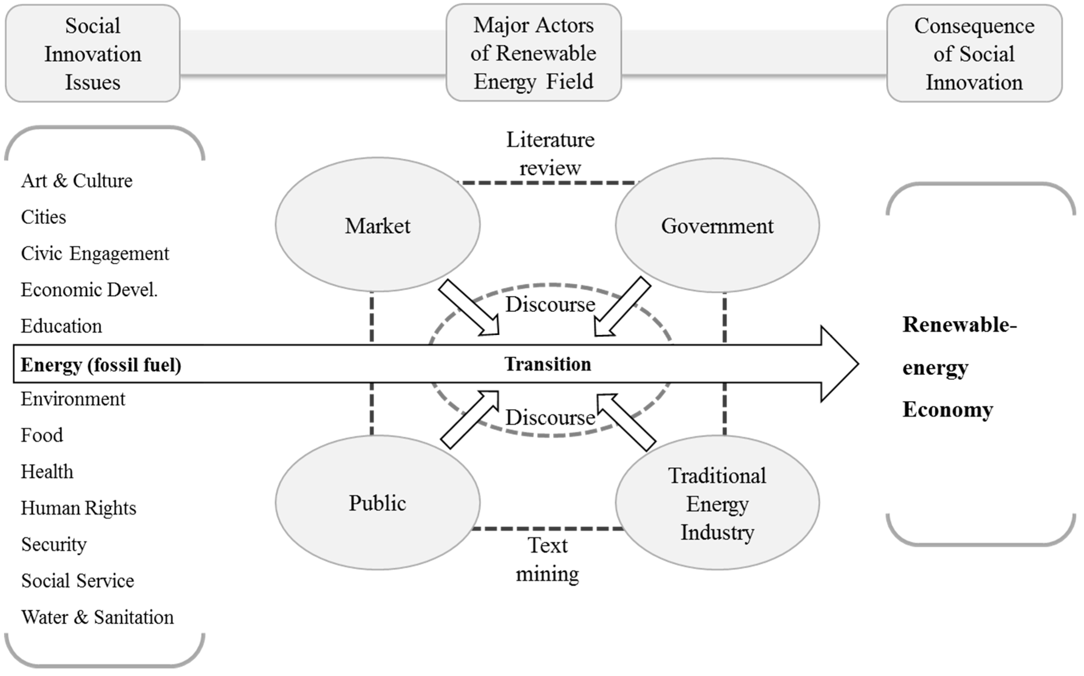There are differences between the literature on social change (e.g., [17,22,27,28,29]), energy transition (e.g., [25,30,31]) and renewable energy (e.g., [24,32,33,34]) in terms of their study settings, scope, themes and interests. Nonetheless, they commonly focus on the transition towards a better society: discussing the requirements of a constantly evolving and collective process involving multiple actors in society and utilizing social learning to address societal challenges and/or needs. Therefore, a fundamental task is to identify those actors who may affect the transition to a renewable-energy economy. Based on the literature, five actors can be distinguished: government, the public, markets, the ‘third’ sector and the traditional energy industry (see Table 1). The current study, however, excludes the influence of the ‘third’ sector for the following reasons: this sector includes various stakeholders that differ substantially across the literature; even though the ‘third’ sector can be regarded as having specific interests—mainly those of non-governmental (NGOs) and other non-profit organizations (NPOs) combined in different various ways—it is problematic to measure the influence of the third sector comprehensively; at the conceptual level, it is nevertheless feasible to measure the influence of each actor within the ‘third’ sector. Indeed NGOs, as a representative of the ‘third’ sector, are a prominent actor that substantially affects energy transition [35,36]. However, measurements of their influence have been inconsistent in the extant literature (i.e., measurements can be based the number of reports published by NGOs [37], NGO funding [38], the workforce employed by the NGO, etc.). Moreover, most NGOs are active globally; their influence is not limited to one country or region. Thus, measuring their influence at a national level tends to be limited to perceived recognition.

Table 1. Literature review: Major actors and reality-based text-mining analysis.

Scope	Theme	Study	Actors
			Government	Public	Market	Third Sector	Traditional Energy Industry
Broad	Social Change	Avelino and Wittmayer [17]	×	×	×	×
		Rana et al. [29]	×	×	×	×
		BEPA [27]		×	×	×
		Geels [39], Coenen et al. [40]	×	×		×
		Grin et al. [28]	×	×	×
		Kemp et al. [22]	×
Middle	Energy Transition	Mallett [30]		×	×	×	×
		Sarrica et al. [25]		×
		Geels [31]		×	×		×
Narrow	Renewable Energy	Wüstenhagen et al. [41]		×	×		×
		Hancock [35]	×			×	×
		Betsill and Stevis [24]		×		×	×
		Michalena and Hills [32]	×	×		×	×
		Hills and Michalena [33]	×		×
		Mazzucato and Semieniuk [34]	×	×			×
		Park [42]	×	×	×

Notes: Government includes states, governments, public agencies, politicians, policy-makers, bureaucrats, local governments and sub-governmental organizations, etc.; Public includes communities, households, families, residents, neighbors, civil societies, community groups and academia, etc.; Market includes markets, firms, businesses, consumers, infrastructure and bank groups; Third sector includes NGOs, non-profit associations, activists, volunteers, benefactors, researchers and philanthropists, etc.; Traditional energy sector includes energy companies, coal mining, oil and gas companies, trade associations, etc.

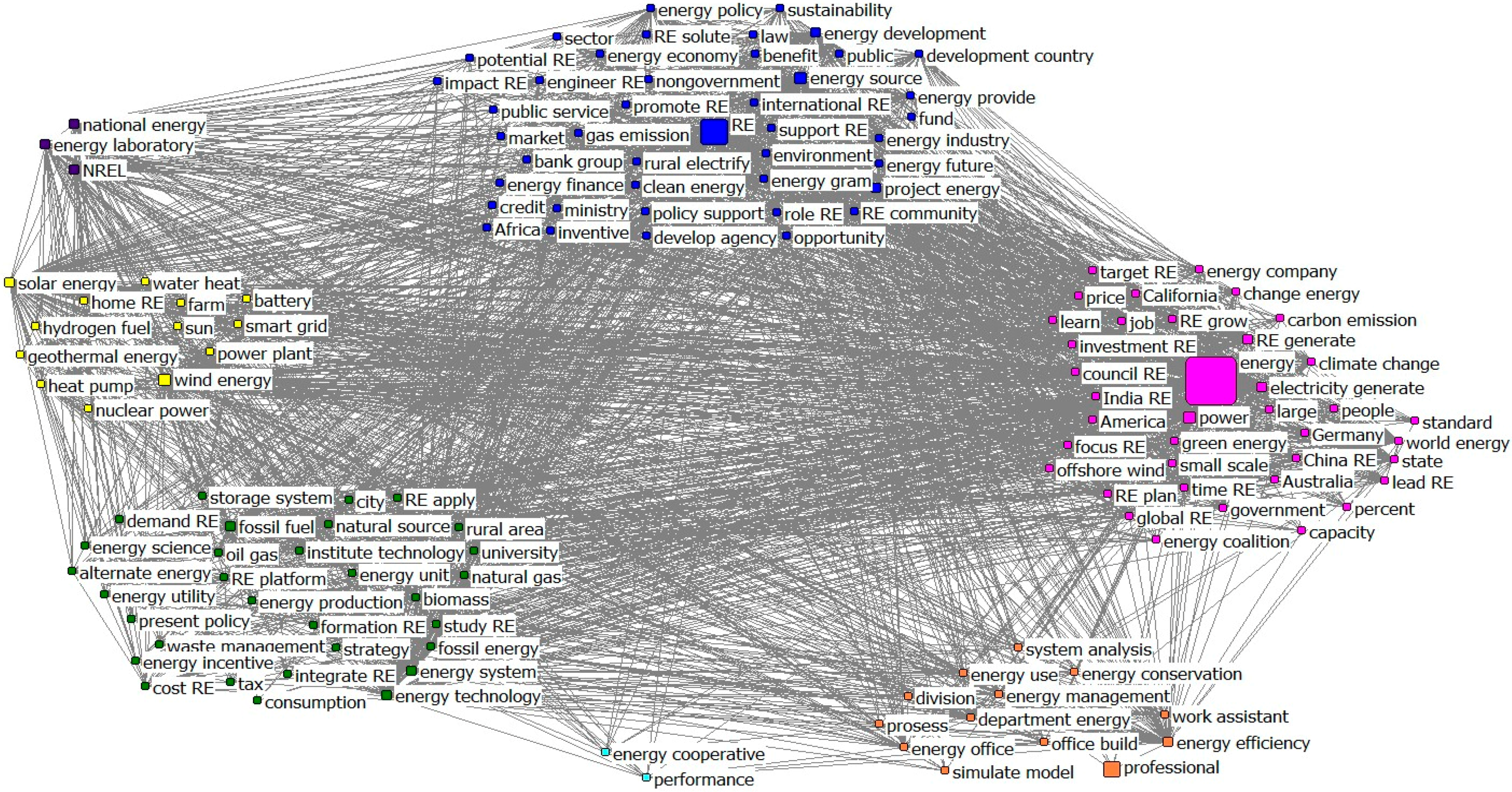
Discourse, meaning written and spoken communications by actors, can promote actors’ efforts to tackle societal issues that need to be resolved in order to achieve a better society [23,24,25,26,30]. The discovery of actors in the texts is becoming increasingly important to research on social innovation. Therefore, we use text-mining analysis to determine which keywords are attributed to each actor within the literature. Using a software module written in Python, we gathered texts on renewable energy for the period 1991–2016 from Google, which is the most comprehensive search engine worldwide and the most efficient channel for discourse analysis. The Google search returned 6.8 billion pieces of information related to renewable energy; narrowing the range of news and documents returned 265 million hits. From the results, we identified 104,644 words that directly related to renewable energy after text cleaning. Text mining was then performed, based on the TF–IDF (Term Frequency–Inverse Document Frequency) and degree centrality value of these words, giving a final list of approximately 140 words (for the formulas and results of text mining, refer to Appendix A and Table A1 of Appendix B, respectively).

Overall, the results of text mining analysis confirm that various keywords formed by the discourse can be classified among the four actors distinguished above (see Table 2). In particular, the law can be regarded as a necessary regulatory system in relation to the phrase “renewable energy.” On the other hand, the two energy-related departments (“Department of Energy” and “ministry”) with lower centrality in terms of the TF–IDF are less critical. Regarding market actors: the phrases market, bank group, energy economy, RE (renewable energy) platform, firm and energy finance appeared to be relatively significant. In the public actor group: public services, renewable energy communities and people appeared to be significant. Finally, within the traditional energy sector, the terms fossil fuel, energy industry and oil and gas are relatively significant. The terms energy companies, natural gas and nuclear power, were slightly less important compared to their frequency of occurrence.

Table 2. Text-mining analysis using renewable energy as a keyword.

Actors	Included Words
Government	energy policy (17/15), state (23/19), department of energy (27/63), policy support (44/37), government (46/29), law (100/89), ministry (137/139)
Market	market (50/44), investment RE (37/48), bank group (77/56), energy economy (78/73), tax (86/124), RE platform (101/90), firm (104/91), energy incentive (107/140), price (125/119), energy finance (131/126)
Public (Civil Society)	job (40/81), institute technology (68/61), public service (89/76), RE community (95/83), energy coalition (106/103), council RE (120/129), public (136/132), people (138/109), association (139/137)
Traditional Energy Industry	fossil fuel (14/12), energy company (30/23), natural gas (32/45), energy industry (35/28), oil gas (73/68), nuclear power (99/102)

Notes: The numbers in parentheses denote term frequency-inverse document frequency (TF–IDF) and degree centrality ranks in order.

Taking into account the aforementioned points from the literature review and text-mining analysis, we identified government, market, public and industry (traditional energy industry) actors as having important influence on the transition to a renewables-based economy.

Government (governmental agencies), as one of the most potent extrinsic forces [43], initiates and guides a variety of policies (technology-push and demand-pull) to promote and achieve current and future deployment goals towards an energy transition [44]. Policies are outcomes of interactions between government and various interest groups or actors within a society and play an important role in providing a collective strategic direction (roadmap) in promoting social change. In this context, policies make contributions to creating and supporting room for niches and experiments (such as development of infrastructure and provision of locations for experimentation-enabled innovation) [3,45,46,47], increasing the attractiveness of the renewables market [48], attracting the private sector to invest in renewable energy by increasing risk-sharing by the government and changing the concerns and uncertainties of the risk–return relationship in the field [49,50] and promoting the collective entrepreneurial efforts of those innovative stakeholders in a society who are unable to exploit their full innovation potential without public intervention [51,52]. This enhances the shared ‘problem frame,’ defined as problem-solving activities [6] in social learning—the integration of knowledge, values and interests from multiple actors that enables joint or collective action to address the challenges involved [53,54], such as the depletion of fossil fuels, the risks of nuclear power and climate change and enabling the transition to a low-carbon, sustainable and renewable-energy economy.

Civil society—a crucial actor in transition [55] processes, comprising the public or citizens—is potentially implicated in processes of socio-technical change as a network of political actors that welcomes or resists technological development in general, or in particular places and settings. Although some scholars consider that the roles and functions of civil society in transition are not clearly defined [56] or are negative [57], the public can aspire toward green living and sustainability, which is normally triggered by societal awareness of environmental and sustainability issues. Such public concerns provide a normative message that the society socially accepts [41,58] and diffuses [59] renewable energy innovation; supports and encourages the use of energy generated from renewable sources [60]; demands and pushes for changes in the sensitivity of economic agents toward environmental solutions [59,61]; and lobbies and protests to unsettle the regime and to influence the policies and procedures of other players [59,62]. According to Avelino and Wittmayer [63], in doing so, civil society actors take the initiative in seeking opportunities to support the ongoing transition to a renewable-energy economy, which in turn tends to boost the formation of public discourse, promote social consensus (or the formation of social norms) on the issue and promote a variety of efforts that are required for transitioning toward social betterment. This means that the public is the most important social force in finding new solutions to issues of social innovation, such as the transition to a renewable-energy economy.

Market actors consist of firms that seek business opportunities by bringing their new products and services to the market served and by implementing business strategies to take advantage of their new development [45,64]; consumers that seek benefit by purchasing satisfactory products and services [65]; and other stakeholders who are interested in investing in some activities [41]. This implies that such economic benefit-seeking behaviors represent the market attractiveness of products and services. Market attractiveness, defined as market potential, is a function of the size and rate of market growth [66], which ensures higher profits [67]. Today, consumers increasingly have positive attitudes towards and express strong demand for renewable energy, which seems to be making a long-term impact on energy markets, by promoting the transition to a green energy market. Furthermore, discerning consumers are finding new means of procuring renewable power to contribute to sustainability ambitions [68] and acting as co-producers, peers and partners in the electricity sector [69]. Hence, consumer demand for renewable energy is increasing as consumers become active so-called ‘prosumers’ who regard electricity as a commodity and both consume and produce electricity from renewable sources [70]. The increasing market attractiveness of renewable energy, due to positive signs on the demand side, encourages firms involved in the renewable energy technology and product sectors to develop strategies for capturing the profit potential. Increased demand and competition among these firms reinforces the market attractiveness. Such a cycle of ongoing reinforced market attractiveness, as an economic driver, contributes significantly to promoting the transition towards a renewable-energy economy.

The traditional energy sector is an important stakeholder and attempts to define the conditions of its work to legitimize its professional autonomy, involving the professionalization of industry or sector members. Such professionalization expresses normative pressures to keep societal development dependent on fossil fuel, such as via massive propaganda campaigns focused on cheaper price of fossil fuels relative to renewables (that remains relatively immature in that there is significant scope for further cost reductions through innovation) [71] and civil society’s preference for low-cost electricity supply [44] generated by fossil fuels such as coal, oil, nuclear, etc. This lobbying effect [72] promotes higher contribution of traditional energy sources to electricity generation and means that the traditional energy sector negatively influences the transition to a renewable-energy economy

The aforementioned points inform the following conceptual framework for tackling the relationships between major actors and the transition to a renewable-energy economy as a social innovation issue (see Figure 1).

Figure 1. Conceptual Framework. The social innovation issues were obtained from the Stanford Social Innovation Review (http://ssir.org) and the authors created a framework based on the literature review and text mining.

3. Model Specification and Methodology

Taking into account the points derived from the literature review, we employ the following panel data model to investigate how multiple actors or agents may affect the transition:

$$RETR{A}_{i,t}=\alpha +\beta {\mathrm{X}}_{i,t}^{\prime }+{\eta }_i+{\epsilon }_{i,t}$$

(1)

where $i$ is the country (N = 25 countries, see Table 2), $t$ is the year (between 1990 and 2014), ${\eta }_i$ denotes the country-specific effect for the $i\mathrm{th}$ individual in the panel (non-observable specific effects) and ${\epsilon }_{i,t}$ is the error term assumed to be independently distributed across $i$ and $t$ with a mean of zero and variance ${\sigma }^2>0$ distributed independently of the regressors (${\mathrm{X}}_{i,t}^{\prime }$). $RETRA$ is a proxy variable that represents the degree of transition to a renewable-energy economy in each country, measured as the contribution of renewables to total energy supply. ${\mathrm{X}}_{it}^{\prime }$ is a vector of explanatory variables that consists of $EP{S}_{i,t},GH{C}_{i,t},EO{S}_{i,t},EN{S}_{i,t},ENG{S}_{i,t},EC{S}_{i,t},GDPP{C}_{i,t}\mathrm{and}ESEC{U}_{i,t}$. EPS is a proxy variable for government pressure. As one of the strongest extrinsic forces, this can directly facilitate social change. We use a composite index of economy-wide environmental policy stringency (EPS) developed by Botta and Kózluk [73] to measure government pressure. The EPS index is based on the taxonomy developed by De Serres et al. [74], which includes market- and non-market-based components. The market-based component groups market-based policy instruments that assign an explicit price to environmental externalities (taxes: CO2, NOX, SOX and diesel; Trading schemes: CO2, renewable energy certificates and energy efficiency certificates; Feed-in tariffs: solar and wind energy; Deposit and refund schemes), while the non-market-based component clusters command-and-control instruments (Standards: NOX, SOX, PMX emission limits and sulfur content limit (diesel); Government research and subsidies expenditure on renewable energy). $GHC$ is a proxy for informal pressure from the general public, measured in thousands of kilograms of CO2-equivalent total greenhouse-gas emissions per capita (per 1000 people). Greenhouse gases, mostly comprising water vapor, carbon dioxide, methane, nitrous dioxide, ozone, chlorofluorocarbons and hydrofluorocarbons, are directly linked to the climate change phenomenon and global warming. Efforts to tackle global warming and move towards planetary sustainability are mainly focused on reducing greenhouse-gas emissions. $EOS,$ $ENS,$ $ENGS$ and $ECS$ refer to trade association pressures, measured as the contributions of oil, nuclear, natural gas and coal sources to electricity generation. Power exercised by interest groups, including the trade associations of the traditional and nuclear energy industries, increases the shares of fossil- and nuclear-based energy, which can inhibit the development and growth of renewable energy technologies. Given this, we used the contributions of the traditional energy sources (oil, natural gas, coal and nuclear) for electricity generation as proxies for the power exerted by their respective trade associations within energy technology industries. $GDPPC$ refers to market attractiveness, derived from both market size and the rate of market growth of renewable energy technologies, driven by consumption of renewable energy technologies (measured in GDP per capita) [60,75]. $ESECU$ denotes a country’s dependency on imported energy, measured as the ratio of imported to total energy supply [60]. Our motivation for including this factor was to control for the relationships between higher import dependency, inducing investment in a country’s own renewable sources and increasing the contribution of renewables to total energy supply (increasing energy security).

Data on $RETRA$ were obtained from the International Energy Agency’s Renewable and Waste Energy Supply section and the US Energy Information Administration’s International Energy Statistics. Data on $EPS$, $GHG$, $EOS$, $ENS$, $ENGS$, $ECS$, $GDP$ and $ESECU$ were extracted from the World Development Indicator database of World Bank. All variables of interest in this study were measured for the 25 OECD countries from 1990 to 2014. However, incomplete data availability means the data set is unbalanced (Australia, Canada, France, Italy, Japan, Korea, Turkey, UK and USA: 1990–2014; Austria, Belgium, Denmark, Finland, Greece, Ireland, Netherland, Norway, Spain, Sweden and Switzerland: 1990–2012; Germany, Hungary and Portugal: 1991–2012; Czech Republic and Slovakia: 1993–2012). We selected the period and countries based on data availability. All variables are expressed in logarithmic form. GDP was calculated according to constant 2009 prices and international purchasing power parity levels.

In the panel context, we conducted the empirical analysis in the following way. We confirmed the characteristics of the data before establishing the empirical model, by testing the presence of normality (in each variable), multi-linearity (between independent variables), structural breaks (in the individual time series), cross-sectional dependence (between cross-sectional units within the panel), homoscedasticity (within cross-sectional units) and autocorrelation (in the panel). We then performed panel unit-root tests to check each variable for stationarity, taking into account the results of structural break and cross-sectional dependence tests. When the series was non-stationary (which means that panel unit-roots existed in each variable) from panel unit-root tests and the sample size was sufficiently large, we conducted a panel co-integration test, considering the results of structural break and cross-sectional tests. In the final phase, we established an empirical to test the relationship between the variables in question based on the results for various panel framework tests, along with consideration of the sample size and conducted the empirical tests.

4. Empirical Analysis

4.1. Panel Estimator

The current study carried out Jarque and Bera’s [76] test for normality. The results revealed that, with some exceptions (Italy, Korea and Norway in $RETRAO$; Denmark and Greece in $EPS$; Belgium and USA in $GHG$; France, Sweden, Switzerland, Turkey and UK in $EOS$; Japan and Norway in $ENS$; Japan and Sweden in $ENGS$; Korea, Portugal, Switzerland, Turkey and USA in $ECS$; Czech Republic, Germany, Italy and Japan in $ESECU$), the individual time-series do not deviate significantly from the normal distribution at 1% or 5% significance levels (the results are available upon request from the authors). Table 3 presents descriptive statistics of the variables in question.

Table 3. Descriptive statistics.

Country	RETRA		EPS		GHG		EOS		ENS		ENGS		ECS		GDPPC		ESECU
	Mean	SD	Mean	SD	Mean	SD	Mean	SD	Mean	SD	Mean	SD	Mean	SD	Mean	SD	Mean	SD
Australia	9.750	1.954	1.537	1.098	24.692	0.874	1.482	0.554	0	0	11.730	4.978	77.286	6.195	30,777.290	18,859.340	−122.746	27.254
Austria	70.468	3.674	2.238	0.644	10.302	0.536	3.197	1.209	0	0	16.435	2.283	11.423	2.576	31,881.840	11,871.060	67.297	2.183
Belgium	4.040	3.665	1.449	0.796	13.862	1.337	1.509	0.784	56.721	3.085	20.893	8.220	16.889	7.789	29,892.770	11,340.950	75.508	1.687
Canada	62.159	1.509	1.697	1.298	22.245	1.194	2.250	0.804	15.053	1.778	5.790	2.646	15.798	3.005	30,177.250	13,854.400	−50.139	7.816
Czech Republic	4.578	1.950	1.589	0.916	14.251	0.804	0.509	0.328	26.361	5.926	1.609	0.544	67.202	6.852	11,053.270	7002.182	24.339	3.100
Denmark	18.776	13.774	2.613	0.814	13.666	1.786	6.241	4.073	0	0	15.983	7.803	59.252	18.052	38,892.840	15,209.630	−14.355	33.586
Finland	31.037	4.715	2.088	0.870	14.103	1.086	1.360	0.788	30.753	2.362	12.559	2.631	24.184	4.692	31,637.090	12,440.790	54.586	3.033
France	14.202	1.937	2.021	1.127	8.984	0.805	1.339	0.603	77.135	1.741	2.468	1.454	5.369	1.632	29,637.510	9720.321	48.002	1.633
Germany	11.857	7.552	2.456	0.501	12.641	1.089	1.484	0.498	25.615	4.999	10.392	2.468	50.892	4.693	32,115.320	9336.628	58.776	2.795
Greece	10.233	3.607	1.641	0.460	11.019	0.790	16.867	3.971	0	0	10.205	8.671	63.150	7.520	16,229.570	8598.137	62.784	3.154
Hungary	3.049	3.101	1.514	0.989	7.335	0.614	7.883	6.405	40.322	3.751	24.756	8.858	24.073	4.346	6927.478	4976.804	53.817	5.792
Ireland	8.108	4.992	1.235	0.693	16.187	1.674	12.739	7.225	0	0	41.460	12.890	38.028	11.667	32,590.590	18,426.950	80.400	10.263
Italy	23.147	7.345	1.940	0.710	9.053	0.851	28.142	17.994	0	0	35.552	13.494	14.045	2.802	25,815.260	9032.672	81.626	2.308
Japan	11.196	1.366	1.757	0.673	10.686	0.329	18.733	6.652	22.994	9.411	25.311	6.391	22.873	6.095	37,835.240	5603.120	82.875	4.620
Korea	1.738	0.842	1.799	1.155	10.930	2.010	11.579	8.374	36.673	6.147	15.095	5.035	34.874	9.721	14,203.580	7372.544	81.906	2.396
Netherlands	6.366	3.933	2.141	0.946	13.809	1.190	2.771	1.055	4.178	0.601	57.176	2.763	29.672	4.441	33,199.780	13,810.640	15.037	8.151
Norway	99.446	1.087	1.670	0.833	11.801	0.513	0.013	0.010	0	0	0.698	1.161	0.086	0.017	51,454.190	28,543.370	−666.472	105.870
Portugal	35.213	9.398	1.688	0.658	7.220	0.700	19.219	11.029	0	0	15.670	12.504	31.187	6.392	14,756.230	6232.670	82.073	2.983
Slovakia	17.375	2.358	1.359	0.783	9.443	0.650	2.721	1.324	52.009	5.102	8.255	1.783	20.400	4.255	9324.929	6080.582	66.696	3.573
Spain	20.648	5.641	2.050	0.723	8.603	0.936	7.589	2.056	26.867	6.504	15.579	13.022	29.694	9.779	19,600.900	9086.922	71.984	531
Sweden	51.561	5.374	2.065	0.896	7.659	0.752	1.659	1.087	45.382	4.405	0.530	0.376	1.808	0.609	36,153.390	12,913.790	34.949	2.479
Switzerland	59.135	2.087	2.272	0.503	7.304	0.421	0.451	0.316	40.747	2.114	1.213	0.268	0.004	0.015	50,481.980	17,045.190	53.811	2.236
Turkey	31.350	8.780	0.995	0.630	4.799	0.725	4.954	2.740	0	0	34.824	13.049	29.930	3.874	5398.555	4632.277	64.550	8.080
UK	5.547	4.992	1.781	1.077	11.685	1.647	3.077	2.953	22.034	4.048	30.122	13.825	39.458	11.109	30,333.750	11,431.970	2.239	22.020
USA	10.851	1.519	1.609	0.803	24.148	1.605	2.546	1.123	19.435	0.541	18.194	5.073	49.426	4.617	36,020.280	11,872.710	21.565	5.503

Notes: A mean value of ENS means that the country does not use nuclear power for electricity generation. A negative value of ESECU indicates that the country is a net exporter.

We then performed Brown et al.’s [77] cumulative sum of recursive residuals (CUSUM) and cumulative sum of recursive residuals of squares (CUSUMQ) tests to detect whether: (a) the regression coefficient estimates show systematic variation over the long term; and (b) deviations from the short-term constancy of regression coefficients are randomized. With the exception of the results of the CUSUM test for Germany and the CUSUMQ test for Australia, Japan, the Netherlands and Switzerland, the two tests’ results showed that almost all the series are stable (the results are available upon request from the authors).

We conducted a multicollinearity test to confirm whether or not independent variables are correlated. As presented in Table 4, the results confirm that the data do not display multicollinearity, demonstrating that all independent variables meet the criteria that VIF is < 10 and that the tolerance value is >0.1 [78,79].

Table 4. Correlation between independent variables.

Panel A: Correlation
	$EPS$	$GHG$	$EOS$	$ENS$	$NGS$	$ECS$	$GDP$	$ESECU$
$EPS$	1.000
$GHG$	−0.054	1.000
$EOS$	0.693	0.346	−1.000
$ENS$	−0.234	−0.191	−0.272	1.000
$ENGS$	−0.005	−0.166	−0.019	−0.286	1.000
$ECS$	0.180	−0.028	0.089	0.127	−0.372	1.000
$GDPPC$	−0.167	0.045	−0.261	0.079	−0.358	0.067	1.000
$ESECU$	0.029	−0.139	−0.200	0.214	0.241	0.247	0.217	1.000
Panel B: Multicollinearity
VIF	3.010	2.790	1.410	2.130	1.480	2.660	4.270	1.800
Tolerance	0.332	0.358	0.707	0.468	0.676	0.375	0.234	0.556

Notes: VIF = variance inflation factor.

We used Wooldridge’s [80] test for the presence of autocorrelation in the panel data, which detected signs of autocorrelation of one order (F statistic = 23.305, $p<0.001$). We performed a panel group-wise heteroscedasticity test, which showed that heteroscedasticity within cross-sectional units exists, rejecting the null hypothesis (at the 1% significance level) of homoscedasticity within cross-sectional units with a Wald test statistic of 5370 ($p=0.001$).

We tested for cross-sectional dependence (CD) using the method proposed by Pesaran [81]. The CD test for fixed-effects regression residuals in each country rejects the null hypothesis of no cross-sectional dependence, showing residual mean absolute correlations (0.475, Pesaran CD statistic 2.192 ($p=0.028$)) (for correlation matrix of residuals of Pesaran’s [81] test, see Table A2 of Appendix C). We used Pesaran’s [82] panel unit-root test, which allows for cross-sectional dependence, to investigate whether the series are stationary. The results in Table 5 indicate that the variables included in the prediction model must be first-differenced before being used in further statistical analysis, showing that the series are non-stationary.

Table 5. Panel unit-root tests.

Variables	With Trend			Without Trend
	Statistic	p-Value	Lag	Statistic	p-Value	Lag
$RETRA$	1.581	0.943	3	$-$0.026	0490	2
$\Delta RETRA$	$-$3.847	0.000	3	$-$8.732	0.000	1
$EPS$	$-$3.272	0.001	2	1.246	0.894	2
$\Delta EPS$	$-$3.390	0.000	2	$-$6.085	0.000	1
$GHG$	2.653	0.996	2	3.087	0.999	2
$\Delta GHG$	$-$9.510	0.000	1	$-$7.978	0.000	1
$EOS$	$-$1.300	0.097	3	$-$1.067	0.143	3
$\Delta EOS$	$-$4.259	0.000	3	$-$2.536	0.006	3
$ENS$	8.517	1.000	2	8.323	1.000	2
$\Delta ENS$	$-$2.273	0.012	1	$-$3.150	0.001	1
$ENGS$	0.516	0.697	3	$-$0.447	0.697	3
$\Delta ENG\mathrm{S}$	$-$3.726	0.000	2	$-$4.746	0.000	2
$ECS$	0.377	0.647	3	3.134	0.999	3
$\Delta ECS$	$-$4.148	0.000	2	$-$7.424	0.000	1
$GDPPC$	1.211	0.887	3	2.502	0.994	3
$\Delta GDPPC$	$-$4.305	0.000	1	$-$3.559	0.000	1
$ESECU$	2.095	0.982	3	3.201	0.999	3
$\Delta ESECU$	$-$5.628	0.000	1	$-$5.584	0.000	1

Notes: The numbers denote the Pesaran cross-sectional augmented Dickey-Fuller (CADF) test z [t-bar] statistics. To remove cross-sectional dependence, the standard DF (or ADF) regressions are augmented with the cross-sectional average of lagged levels and the first differences of the individual series (CADF statistics). The lag lengths for the panel test [in square brackets] are based on those employed in the univariate ADF test. The normalized z-test statistic is calculated using the t-bar statistics.

Non-stationarity of the series suggests that there might be a long-term equilibrium among the variables. Hence, we conducted the heterogeneous panel co-integration tests proposed by Westerlund [83], which allow for cross-sectional dependence. However, it was not possible to conduct the co-integration tests, due to the large number (>6) of covariates and the small sample size relative to the number of variables to be tested.

The presence of first-order autocorrelation in the series indicates that a model that accounts for autocorrelation—the dynamic model (which specifies the dependent variable based on its values in the previous period)—should be used. Also, cross-sectional dependence poses another obstacle to accurate and efficient parameter estimates. Cross-sectional dependence among errors can be eliminated by including time dummies or by cross-sectionally demeaning the data. We created year-dummy control variables to prevent cross-individual correlation [84,85], thereby improving the robustness of our results [86]. It calls for a first-order dynamic panel-data approach to exploring the relationships between the variable in question.

In addition, the results of the panel unit-root tests suggest that the variables included in the prediction model must be first-differenced before being used in further statistical analyses. There can also exist complex dynamic relationships between the variables examined in this study. Almost all economic and social situations, including the situation where society faces the transition to a renewable-energy economy, in which multi-actors are interrelated, are closely related to each other regarding each variable that comprises the system. This implies that all the variables in question, i.e., $RETRA$, $EPS$, $GHG$, $EOS$, $ENS$, $ENGS$, $ECS$, $GDP$ and $ESECU$, capture very complex dynamic interactions that can drive changes in both directions. The presence of such dynamic and interrelated relationships seems to yield reverse causality problems in the panel models.

For modeling, this study uses panel vector autoregressive (VAR) model in the firs differences, allowing us to estimate the underlying dynamic relationships between the variable without applying any a priori restriction. The panel VAR model in the first difference can be expressed as follows:

$$\Delta Y_{i,t}=\gamma \Delta Y_{i,t-1}+\beta \Delta {\mathrm{X}}_{i,t}^{\prime }+\Delta {\epsilon }_{i,t}+d_t$$

(2)

where $\Delta$ is the first difference operator. $Y_{i,t}$ is a vector of the logs of dependent variables. ${\mathrm{X}}_{i,t}^{\prime }$ is a vector of the logs of exogenous control variables. ${\epsilon }_{i,t}$ is a vector of idiosyncratic errors and $d_t$ is the time dummy. The vectors of dependent and exogenous control variables consist of $RETRA$, $EPS$, $GHG$, $EOS$, $ENS$, $ENGS$, $ECS$, $GDP$ and $ESECU$.

For Equation (2), differencing introduces a simultaneity problem, because the lagged endogenous variables on the right-hand side correlate with the new differenced error term. Genuine errors across the industries are characterized by heteroscedasticity. These conditions led us to use the instrumental variable (IV) [87] or generalized method of moments (GMM) estimators—specifically, the difference GMM [88] and system GMM [89,90]—to infer a causal relationship among the variable in question.

However, both the IV and GMM estimator techniques suffer from a problem: under certain conditions, the variance of the estimates might increase asymptotically, generating considerable bias.

This problem occurs if the sample is finite, as in this study [90]. When $T\left(time\right)\to \infty$, the least squares dummy variable (LSDV) estimator is consistent and is biased only to a negligible degree [91]. However, when $T$ < 30, Judson and Owen [92] show that the LSDV estimator has a bias of up to 20% of the time value coefficient of interest. When $T$ < 30, as in this study, a bias-corrected LSDV (LSDVC) estimator performs well, compared to the IV or GMM estimation techniques by Judson and Owen [92] for balanced panel and Bruno [93] (for unbalanced panel) in terms of bias and root-mean-square error. Hence, we applied the LSDVC estimator, including it in Equation (2), causality, complex dynamic relationships between the variables, is determined by running Wald tests on the coefficients of variables.

4.2. Empirical Results

We obtained the results from the five estimators, difference GMM, system GMM, LSDVC (Anderson–Hsiao (Initial A), Arellano–Bond (Initial AB) and Blundell–Bond (Initial BB)). The results from LSDVC estimators are presented in Table 6, Table A3 and Table A4 of the Appendix D and are similar regarding estimated parameters and corresponding p-values but the AB estimator is more efficient [94] (for the results from difference and system GMMs, see Table A5 and Table A6 of the Appendix D, which is for comparison with the LSDVC estimation results).

Table 6. Panel Vector Auto regression Results (Bias-Corrected LSDV Estimation Initially Utilizing Anderson-Bond Estimator).

Panel A: Bias-Corrected LSDV Estimation
Independent Variables	Dependent Variables
	$\mathbf{\Delta }\mathit{R}\mathit{E}\mathit{T}\mathit{R}{\mathit{A}}_{\mathit{i}\mathit{t}}$	$\mathbf{\Delta }\mathit{E}\mathit{P}{\mathit{S}}_{\mathit{i}\mathit{t}}$	$\mathbf{\Delta }\mathit{G}\mathit{H}{\mathit{G}}_{\mathit{i}\mathit{t}}$	$\mathbf{\Delta }\mathit{E}\mathit{O}{\mathit{S}}_{\mathit{i}\mathit{t}}$	$\mathbf{\Delta }\mathit{E}\mathit{N}{\mathit{S}}_{\mathit{i}\mathit{t}}$	$\mathbf{\Delta }\mathit{E}\mathit{N}\mathit{G}{\mathit{S}}_{\mathit{i}\mathit{t}}$	$\mathbf{\Delta }\mathit{E}\mathit{C}{\mathit{S}}_{\mathit{i}\mathit{t}}$	$\mathbf{\Delta }\mathit{G}\mathit{D}\mathit{P}\mathit{P}{\mathit{C}}_{\mathit{i}\mathit{t}}$	$\mathbf{\Delta }\mathit{E}\mathit{S}\mathit{E}\mathit{C}{\mathit{U}}_{\mathit{i}\mathit{t}}$
$\Delta RETR{A}_{it}$		−0.021	−0.003	0.003	−0.002	−0.017 ***	−0.016 ***	−0.001	0.002
$\Delta EP{S}_{it}$	0.074 ***		−0.011 **	0.001	0.003	0.005	0.000	0.021 *	−0.012
$\Delta GH{G}_{it}$	−0.170	−0.410 ***		0.006	0.018	0.043 ***	0.064 ***	0.186 ***	−0.038
$\Delta EO{S}_{it}$	−2.609 ***	0.090	0.396 ***		−0.082	−0.145 ***	−0.291 ***	0.226 *	0.057
$\Delta EN{S}_{it}$	−2.918 ***	−0.762 **	0.019	−0.052		−0.224 ***	−0.277 ***	0.190	−0.022
$\Delta ENG{S}_{it}$	−2.264 ***	0.005	0.353 ***	−0.056	−0.089		−0.312 ***	−0.056	0.033
$\Delta EC{S}_{it}$	−2.910 ***	0.630 *	0.597 ***	−0.051	−0.094	−0.251 ***		−0.196	0.083
$\Delta GDPP{C}_{it}$	0.074 *	0.200 ***	0.055 ***	−0.007	0.007	−0.007	−0.002		0.023
$\Delta ESEC{U}_{it}$	0.009	0.123	−0.034 *	0.006	0.012	0.015	0.022 **	−0.000
Each dependent variable in period, $t-1$	0.762 ***	0.812 ***	0.762 ***	1.000 ***	1.078 ***	0.820 ***	0.820 ***	0.919 ***	0.980 ***
Panel B: Statistical Values for Panel Causality Tests
Independent Variables	Dependent Variable
	$\mathbf{\Delta }\mathit{R}\mathit{E}\mathit{T}\mathit{R}\mathit{A}$	$\mathbf{\Delta }\mathit{E}\mathit{P}\mathit{S}$	$\mathbf{\Delta }\mathit{G}\mathit{H}\mathit{G}$	$\mathbf{\Delta }\mathit{E}\mathit{O}\mathit{S}$	$\mathbf{\Delta }\mathit{E}\mathit{N}\mathit{S}$	$\mathbf{\Delta }\mathit{E}\mathit{N}\mathit{G}\mathit{S}$	$\mathbf{\Delta }\mathit{E}\mathit{C}\mathit{S}$	$\mathbf{\Delta }\mathit{G}\mathit{D}\mathit{P}\mathit{P}\mathit{C}$	$\mathbf{\Delta }\mathit{E}\mathit{S}\mathit{E}\mathit{C}\mathit{U}$
$\Delta RETRA$		0.530	0.350	0.080	0.010	20.040 ***	18.010 ***	0.020	0.060
$\Delta EPS$	6.320 ***		3.870 ***	0.010	0.030	2.380	0.010	2.780 *	2.050
$\Delta GHG$	1.650	8.610 ***		0.020	0.030	6.210 ***	15.620 ***	9.610 ***	0.840
$\Delta EOS$	112.060 ***	0.100	54.550 ***		0.140	5.650 ***	50.970 ***	3.240 *	0.390
$\Delta ENS$	76.880 ***	3.890 **	0.070	0.190		11.150 ***	42.520 ***	1.220	0.040
$\Delta ENGS$	70.600 ***	0.000	37.180 ***	0.170	0.250		55.890 ***	0.170	0.150
$\Delta ECS$	85.730 ***	2.950 *	77.840 ***	0.120	0.150	12.120 ***		1.500	0.580
$\Delta GDPPC$	2.740 *	19.200 ***	42.590 ***	0.200	0.030	1.570	0.200		2.590
$\Delta ESECU$	0.010	1.440	3.090 *	0.160	0.210	2.280	4.910 **	0.000

Notes: Panel A contains the results of tests based on Bias-corrected LSDV estimates. Time dummies are included in the estimation. Bias is corrected up to the first order, 0 (1/T) and 500 replications are used in the bootstrap procedure to find the asymptotic variance-covariance matrix of estimators. All estimates were controlled to include time effects (not reported in this study). Panel B reports ${\chi }^2$-statistics. In Panel A and B, ***, ** and * denote the 1%, 5% and 10% significance levels, respectively. Each dependent variable in period, $t-1$, denotes $\Delta RETR{A}_{it-1}$, $\Delta EP{S}_{it-1}$, $\Delta GH{G}_{it-1}$, $\Delta EO{S}_{it-1}$, $\Delta EN{S}_{it-1}$, $\Delta ENG{S}_{it-1}$, $\Delta EC{S}_{it-1}$, $\Delta GDPP{C}_{it-1}$, $\Delta ESEC{U}_{it-1}$ in order of estimation presented in Panel A.

As presented in Table 6, seven variables, including one lagged dependent variable, significantly affect the transition to a renewable-energy economy. The LSDVC estimation results of Table 6 show evidence of dynamic effects in all bias-corrected LSDV estimations; the dependent variables (e.g., $\Delta RETR{A}_{it}$, $\Delta EP{S}_{it}$) depend on their values in the previous period (e.g., $\Delta RETR{A}_{it-1}$, $\Delta EP{S}_{it-1}$) at 1% significance levels, by demonstrating that a null hypothesis where each coefficient equals zero can be rejected at 1% significance level and that each coefficient is a positive sign. The results from panel causality tests presented in Panel B of Table 6 find that $EPS$ and $GDPPC$ have positive effects on $RETRA$, that $EOS$ and $ENS$ have negative effects on $RETRA$, that $ENS$ negatively affect $EPS$, that $EOS$ has a positive effect on $GDPPC$, that $ENS$ and $EOS$ negatively affect and $ESECU$ positively affects $ECS$, that $ENS$ and $EOS$ have negative effects on $ENGS$ and that $EOS$ and $ESECU$ have a positive and a negative effect on $GHG$, respectively, at 1%, 5% and 10% significance levels. However, any significant direct relationships between $ENS$ and $EOS$, $EPS$ and $ENGS$, $EOS$ or $\mathrm{ESECU}$, $RETRA$ and $GHG$ or $ESECU$, $GDPPC$ and $ECS$, $ENGS$, $ENS$ or $ESECU$ do not exist (The complex dynamic casual relationships between the variables are also presented through Casual Loop Diagram (see Figure 2) drawn based on the results of LSDVC (Initial AB)-based panel causality tests).

Figure 2. Casual Loop Diagram. P and N stand for positive and negative casual relationships between the variables.

The findings suggest that government (positive sign), market (positive sign) and traditional energy industries (negative sign) are the main factors affecting the transition to a renewable-energy economy and that persistent commitment to renewables is required to promote this transition.

5. Discussion and Conclusions

This study investigated how the main actors influence the transition to a renewable-energy-based economy, using unbalanced panel data for 25 countries spanning the period from 1990 to 2014. We performed some panel framework analyses to evaluate the data characteristics before establishing the panel estimator and empirically testing the relationship between the variables of interest. We used the bias-corrected least squares dummy variables (LSDVC) to control for time dummies in order to eliminate dynamic panel bias and yield more efficient and consistent parameter estimates. The LSDVC dynamic estimator proved to be the most appropriate, taking into account the results of panel framework analyses. We also used other panel estimators, as appropriate, for comparison with the LSDVC estimation results.

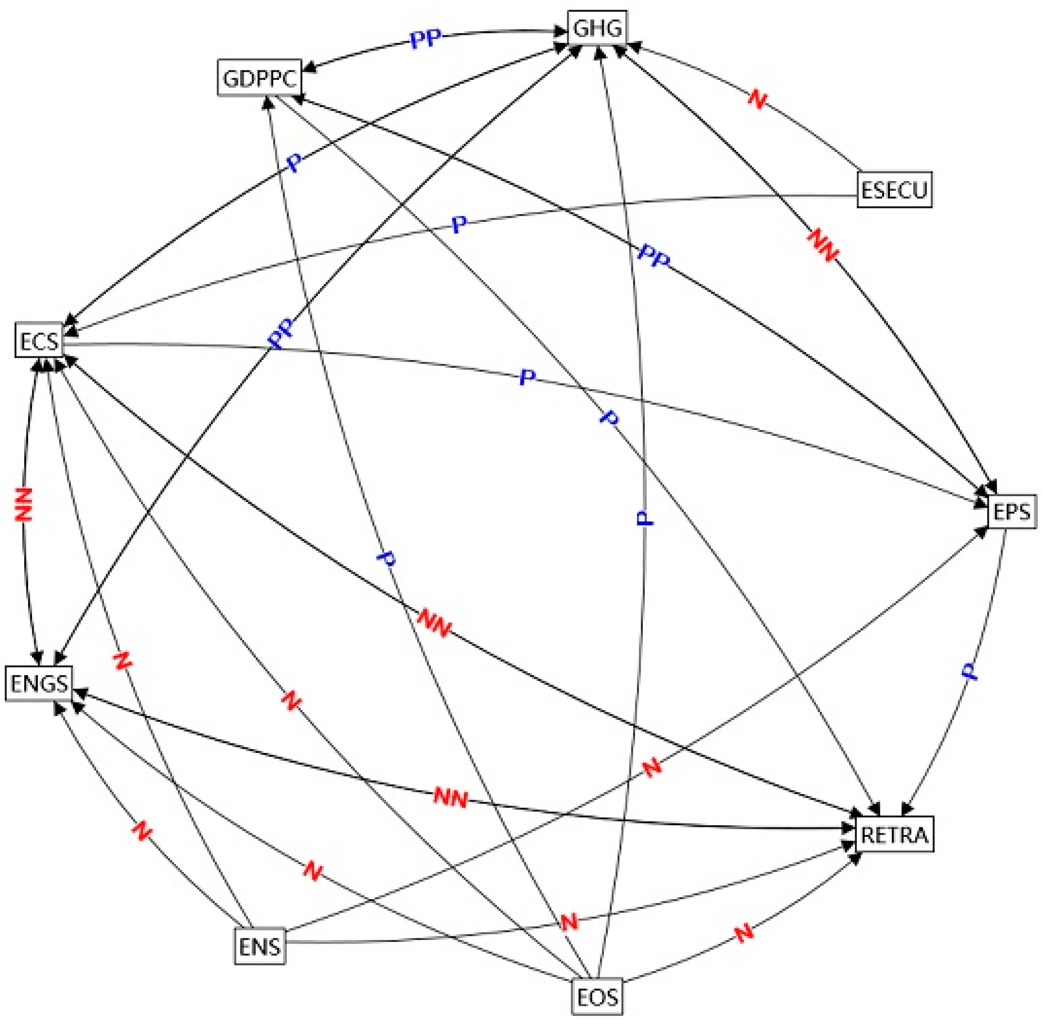
We can draw the following five conclusions based on the LSDVC estimation results from this study. First, the LSDVC estimation results show which of the actors should be prioritized by policy-makers to promote the transition to a renewable-energy-based economy. Based on the coefficients, the variables (most important first) follow the sequence ENS (negative sign) > ECS (negative sign) > EOS (negative sign) > ENGS (negative sign) > RETRA (continuous commitment to renewables; positive sign) > EPS (positive sign) > GDPPC (positive sign). Hence, to promote the transition to renewables, priority should be given to social efforts to decrease the share of traditional energy sources and consumption. These efforts should be followed by policies that ensure steadfast commitment to renewables; that induce economy-wide activities to be eco-friendly; and which develop market conditions that can create massive demand or renewable energy use and renewable energy technologies and products. Overall, the LSDV estimation results show that governments and markets actually induce social efforts to promote the transition to renewables; and that the traditional energy slows the transition to a renewable-based economy.

Second, the findings from the LSDVC estimation show that the traditional energy industries negatively affect the transition to renewables, in which a nuclear source for electricity has emerged as having the most negative influence, followed by coal, oil and natural gas sources for electricity. This implies that existing energy production, consumption and management systems based on traditional energy sources can be an encumbrance to the deployment of renewable energy in society. However, these findings do not necessarily mean that traditional energy sectors represent an obstacle to the process of transitioning to a renewable-energy economy. Rather, it implies that this sector can be the largest strategic reference point towards which each government needs to expend a great deal of effort in promoting social innovation towards renewables. Although modern societies currently face the depletion of fossil fuels, the risks associated with nuclear power and climate change are formidable societal challenges. The core infrastructures used by the private and public sectors of society are still heavily dependent on traditional energy derived from fossil fuels. Achieving a renewable-energy economy will take a long time. This implies that governments should take a gradual, long-term approach to creating various socially innovative activities, such as the transformation and downscaling of reliance on traditional forms of energy, public infrastructure and the energy deployment system itself. Such efforts require a variety of economy-wide market- and nonmarket-based instruments. This study also shows that negative bidirectional casual relationships between RETRA and ECS or ENGS exist. According to Rubio-Maya et al. [95], the high productivity of electricity production from fossil fuels like coal and natural gas still hinder the utilization of renewable energy technologies. In this context, the results suggest that the production of electricity through the cheapest fossil fuels interferes with the production of electricity from renewable energy sources and that the active use of renewable energy can reduce the use of coal and natural gas. Should this occur, investments made into developing natural gas could be invested in renewable energy production technology. This study shows that, predictably, there are positive bidirectional casual relationships between GHG and ECS or ENGS and that ESECU has a positive influence on ECS and negative effects on GHG. The results imply that among traditional energy sources, natural gas, nuclear, oil and coal negatively affect the transition to renewable-energy economy. Coal in particular is directly related to energy security, which delays the transition. That is because coal is widely used in the industry and is a source that better meets four important elements considered in energy security: availability (e.g., market liquidity), accessibility (e.g., supplier diversity), affordability (e.g., economic efficiency) and acceptability (e.g., environmental and societal acceptability), as compared to oil [96]. Our calculation shows that the ratio of coal source for electricity generation from traditional energy sources (oil, coal, natural gas and nuclear) on average in the 25 countries for 1990–2014 is about 41%. This suggests that policy-makers should make efforts to reduce coal consumption.

Third, the findings of this study demonstrate that markets have a significantly positive influence in promoting sustainability and the transition to a renewable-energy economy. This implies that policy-makers should make full use of market functions to encourage the economy to be renewable-friendly by promoting the renewable energy technology sector. The promotion of production and consumption of renewable energy are very important for ensuring market competitiveness and for creating good opportunities and profit structures for potential investors. This means that, in order to establish sustainable development and renewable energy as the basic system of national energy management, in the context of Lewis and Wiser [97] and Sawhney and Kahn [98], each country requires sufficient demand for renewable energy within its domestic markets. Market conditions that create representative demand for renewable energy, including technologies and products—i.e., market attractiveness as a function the size and rate of market growth [66]—depend mainly on sociopolitical and economic contexts, driven by increase in real GDP that allows supporting regulatory costs to promote the deployment of renewable energy [60]. This support framework also requires policies that: promote the dual missions of maximizing business profit while also realizing social justice; create supportive conditions for more local deals in different geographic locations [47]; and spur collective entrepreneurial efforts by innovative stakeholders, especially firms, that would otherwise be unable to exploit their full innovation potential without public intervention [51,52]. Furthermore, it requires awareness and agreement that all members of society should have a responsibility to promote renewable energy for present and future generations and that such investment would stimulate the sustainable economy [99]. In this context, the study findings suggest that it is necessary for the government to properly utilize a mixed combination of sociopolitical and economic mechanisms, not only economic considerations, in promoting the transition to a renewable-energy economy. The results of causality tests also indicate that public and government actors positively interact with market actors, by showing convincing evidence of bidirectional positive interaction between $GDPPC$ and $EPS$ or $GHG$. It suggests that although the market itself may have a positive impact on the transition to a renewable-energy economy, policy-makers should bear in mind that creating interaction between the government and the market [100] and the public discourse network that stimulates the market actors [101] are very crucial to promote the transition to a renewable-energy society. Based on such interactions, policy-makers should make significant effort to enhance their potential synergy effects in developing and implementing a variety of policy instruments for promoting the transition. In the context of Newell et al. [102], this means that policy-makers need to understand the collaborative process at the level of a multi-actor network that transcends the formal hierarchy in order to invest in renewable energy.

Fourth, the results of this study show that governmental actors positively influence the transition to renewables. We used a composite index of economy-wide environmental policy stringency (EPS) as a proxy variable for governmental pressure, based on the perspective that government’s role is expressed as various policies—coercive pressure—to which firms attempt to adapt in order to increase their competitive advantage [43]. The EPS index encompasses a wide range of market- and non-market-based policy instruments that are necessary to make each economy environmentally sound and sustainable, such as taxes on pollutants and fuels; trading schemes for carbon dioxide emissions, renewable energy and energy efficiency; feed-in tariffs for renewables; deposit and refund schemes; limits on pollutant emissions; R&D and subsides for renewable energy. In this context, the findings suggest that governments should take into account both sides of a sociopolitical and economic situation, give consideration to maintaining a balance between the differing interests expressed by actors in society and develop and implement various market- and non-market-based policy instruments for deployment of renewable energy. Furthermore, this study demonstrates that there is a dynamic effect (path dependence), showing that the contribution of renewables to total energy supply in previous periods has positive effects on that in the present period. This suggests the importance of a persistent commitment to renewables. Hence, in order to promote the transition to a renewable-energy economy, various continuous efforts are required across the society. By demonstrating a bidirectional positive causal relationship between $EPS$ that positively affects $RETRA$ and $GDPPC$, the results of causality tests show that environmental policy facilitates the transition to a renewable energy society by interacting with the market. This suggests that policy-makers should make significant efforts to develop and implement reliable policy measures that can enhance high and positive elasticities (elasticity of environmental efforts to market expansion and vice versa) and that synergy effects between the environment and market expansion policies should be taken into account in developing and implementing policy instruments to further promote the transition to renewable-energy economy.

Fifth, this study showed convincing evidence of dynamic effects (dynamic-path dependence) in all LSDVC estimations, by demonstrating that the dependent variables are based on their values in the previous at 1% significance levels. It suggests that a learning-by-doing effect exists in each variable, showing that the value of $ERETRA$, $EPS$, $GHG$, $DEOS$, $ENS$, $ENGS$, $ECS$, $CGDPPC$ and $NESECU$ in the present period depends on their values in the previous period. Such learning-by-doing effects refer to a variety of mechanisms that the current level of the contribution of the renewable energy component to the total energy supply, environmental policy stringency, greenhouse gas emissions, market growth, power generation from the traditional energy sector, or dependence on imported energy might be enhanced by its own previous level. The results of this study suggest that policy-makers should continuously make significant efforts to use industrial export promotion policy strategies by continuously creating productivity gain through exporting and promoting industry expansion as much as possible, implement various policy strategies to promote the transition to a renewable-energy economy by increasing the contribution of renewables to total energy supply, implement environmental policies that encourage firms in the industry to be eco-friendly and reduce the ratio of power generation from traditional sources such as oil, natural gas, nuclear energy and coal. Especially, considering that there are positive bidirectional dynamic relationships between $GDPPC$ and $EPS$ or $GHG$ and that $GDPPC$ and $EPS$ have positive effects on $RETRA$, policy-makers should make and implement an optimum policy-mix of various policy instruments to promote market expansion, environmentally sound and sustainable development of society and public awareness about the environmental sustainability of society and necessity of the transition to renewable-energy economy. Such various government efforts to develop and implement a variety of policy measure need to be undertaken by carefully considering the time lag shown as the result of a dynamic path-dependence process.

Sixth, this study found that public actors do not significantly direct influence the transition to a renewable-energy economy. This does not necessarily mean that the public is not important for this purpose. Rather, the results indicate that, despite the importance of public’s central role in forming discourse regarding the transition, public actors do not exert enough of influence to induce efforts toward tackling the societal issues and challenges related to the renewables transition. This interpretation of the results can be supported by the convergence of iterated correlation (CONCOR) semantic network analysis applied to the text-mining data obtained in Section 2 that we conducted (for details of the results of the CONCOR semantic network analysis, refer to Appendix E). This analysis showed that public-related terms, such as Community, Public and Public service, are centered on “renewable energy,” indicating that public actors appeared to be prominent in forming discourse regarding the transition to a renewable-energy economy. Hence, the results of the panel data and CONCOR semantic network analyses suggest that, even though public actors form strong bonds with each other and a consensus on the transition to a renewable-energy economy, this is still insufficient to encourage various social innovations that can directly contribute to the deployment of renewable energy. However, the result of causality tests that there is a bidirectional positive causal relationship between $GHG$ and $GDPPC$ implies that public actors can indirectly affect interaction between the government and market actors and transition to renewable-energy economy. This suggests that the transition cannot—and should not—be radical but should instead be considered as a process of social innovation that induces gradual change with the participation of various stakeholders and members of society. In this context, the study findings should be understood as indicating that the public is still contributing to the transition in terms of generating discourse on this process and that discourse formed by public actors could mobilize social innovation across society. Taking into account the results of CONCOR analysis and causality tests, public actor is a very important factor indirectly affecting the transition to the renewable-energy society. It suggests that policy-makers need to devise and implement policy strategies to utilize public actors and encourage the market and the government, which leads to promotion of the transition.

This study contributes to a detailed understanding of the many actors who are likely to affect the transition to a renewable-energy economy, through a literature review and text-mining analysis and through empirical examination of the influences of major actors on this transition. However, the inability of the data to measure the components’ forces (for example NGOs, academic groups and investor groups) limits our ability to empirically grasp their effects on the transition to a renewable-energy economy. Hence, further research is required to identify the roles of these components in promoting a transition to a renewable-energy economy. An analysis of the effects of major actors on the transition to a renewable-energy economy can be performed taking various approaches, such as multi-actor, sociopolitical-economy, stakeholder, legitimacy theory. For better understanding of the influences of the actors in the process of the transition, an integrated approach should be done in future research. In addition, the results of the data analysis presented in this study should be viewed with regard to the complexity of the issue, namely, correlations across space, which is especially true for European OECD countries. In terms of stringent environmental policy; greenhouse gas emissions; the market; import dependency of energy; and the contribution of the sum of oil, nuclear, natural gas and coal sources to electricity generation of the sample that consists of European countries only, this study obtained Pesaran CD statistics of 12.379 ($p=0.000$), 24.845 ($p=0.000$), 21.063 ($p=0.000$), 48.932 ($p=0.000$), 3.211 ($p=0.000$) and 11.397 ($p=0.000$), respectively and the corresponding averaged absolute correlation coefficients are 0.263, 0.388, 0.771, 0.228 and 0.295. The test results indicate interactions among European OECD countries for each variable. In particular, the result of the Pesaran CD test for the market (Pesaran CD statistics of 48.932 and average absolute correlation coefficient of 0.771) demonstrates that European OECD countries have a highly linked energy market. If fact, the European energy market is now tightly connected, as a result of three integration packages [103]; package one (1996–1998) allows for the opening of the energy market, package two (2003) unbundles the energy market and package three (2009) newly unbundles the regime and provides clear obligations in terms of national regulations. The consensus on energy issues has led the European Commission to initiate a joint policy response to three themes: sustainability, competitiveness and security of supply. This means that the European Union’s energy policy primarily focuses on the same direction and destination and within this macro framework, each member country pursues a detailed energy policy. The market is thus moving in close alignment with the EU’s overall energy policy. This context is a potential cause for cross-sectional dependence between the countries with regard to the market. However, it is difficult to attribute this highly linked market to only one cause. According to Vega and Maria [104], addressing the nature of the observed correlation across European OECD countries in terms of the market, including other variables, is a complex issue, because potential sources of interactions between countries, space, or regions (namely, spatial autocorrelation) can be a common factor and/or spatial spillover effects may be caused by various factors. Thus, the potential causes of spatial autocorrelation need to be explored in future research so as to obtain more efficient estimates.

References

1. Verbong, G.; Loorbach, D. (Eds.) Governing the Energy Transition: Reality, Illusion or Necessity? Routledge: New York, NY, USA, 2012. [Google Scholar]
2. Geels, F.W. The multi-level perspective on sustainability transitions: Responses to seven criticisms. Environ. Innov. Soc. Transit. 2011, 1, 24–40. [Google Scholar] [CrossRef]
3. Fischer, L.-B.; Newig, J. Importance of actors and agency in sustainability transitions: A systematic exploration of the literature. Sustainability 2016, 8, 476. [Google Scholar] [CrossRef]
4. Wittmayer, J.M.; Avelino, F.; van Steenbergen, F.; Loorbach, D. Actor roles in transition: Insights from sociological perspectives. Innov. Soc. Transit. 2017, 24, 45–56. [Google Scholar] [CrossRef]
5. De Haan, J.; Rotmans, J. Patterns in transitions: Understanding complex chains of change. Technol. Forecast. Soc. 2011, 4, 45–58. [Google Scholar] [CrossRef]
6. Grin, J.; Rotmans, J.; Schot, J. (Eds.) Transitions to Sustainable Development: New Directions in the Study of Long Term Transformative Change; Routledge: New York, NY, USA, 2010. [Google Scholar]
7. Geels, F.W.; Schot, J. The Dynamics of Transitions: A Socio-Technical Perspective. In Transitions to Sustainable Development: New Directions in the Study of Long Term Transformative Change; Grin, J., Rotmans, J., Schot, J.W., Eds.; Routledge: New York, NY, USA, 2010. [Google Scholar]
8. Rotmans, J.; Loorbach, D. Complexity and transition management. J. Ind. Ecol. 2009, 13, 184–196. [Google Scholar] [CrossRef] [Green Version]
9. Anderson, T.; Curtis, A.; Wittig, C. Definition and Theory in Social Innovation: The Theory of Social Innovation and International Approaches; ZSI Discussion Paper, Nr. 33; Zentrum für Soziale Innovation: Wien, Austria, 2015. [Google Scholar]
10. Franz, H.-W.; Hochgerner, J.; Howaldt, J. (Eds.) Final observations. In Challenge Social Innovation (1–16); Springer: Berlin, Germany, 2012. [Google Scholar]
11. Hochgerner, J. New combinations of social practices in the knowledge society. In Challenge Social Innovation; Franz, H.-W., Hochgerner, J., Howaldt, J., Eds.; Springer: Berlin, Germany, 2012. [Google Scholar]
12. Hubert, A. Empowering People, Driving Change: Social Innovation in the European Union; BEPA (Bureau of European Policy Advisers): Brussels, Belgium, 2011.
13. Pol, E.; Ville, S. Social innovation: Buzz word or enduring term? J. Socio Econ. 2009, 38, 878–885. [Google Scholar] [CrossRef]
14. Martinelli, F. Social innovation or social exclusion? Innovation social services in the context of retrenching welfare state. In Challenge Social Innovation; Franz, H.-W., Hochgerner, J., Howaldt, J., Eds.; Springer: Berlin, Germany, 2012; pp. 169–180. [Google Scholar]
15. Mulgan, G. Social innovation theories: Can theory catch up with practice? In Challenge Social Innovation; Franz, H.-W., Hochgerner, J., Howaldt, J., Eds.; Springer: Berlin, Germany, 2012; pp. 19–42. [Google Scholar]
16. Markard, J.; Raven, R.; Truffer, B. Sustainability transitions: An emerging field of research and its prospects. Res. Policy 2012, 4, 955–967. [Google Scholar] [CrossRef]
17. Avelino, F.; Wittmayer, J.M. Shifting power relations in sustainability transitions: A multi-actor perspective. J. Environ. Pol. Plan. 2016, 18, 628–649. [Google Scholar] [CrossRef]
18. Newell, P.; Mulvaney, D. The political economy of the ‘just transition’. Geogr. J. 2013, 179, 132–140. [Google Scholar] [CrossRef]
19. Baker, L.; Newell, P.; Phillips, J. The political economy of energy transitions: The case of South Africa. New Political Econ. 2014, 19, 791–818. [Google Scholar] [CrossRef]
20. Jenkins, K.; Heffron, R.J.; McCauley, D. The political economy of energy justice: A nuclear energy perspective. In The Palgrave Handbook of the International Political Economy of Energy; Palgrave Macmillan: London, UK, 2016. [Google Scholar]
21. Smith, A.; Stirling, A.; Berkhout, F. The governance of sustainable socio-technical transitions. Res. Policy 2005, 34, 1491–1510. [Google Scholar] [CrossRef]
22. Kemp, R.; Loorbach, D.; Rotmans, J. Transition management as a model for managing processes of co-evolution towards sustainable development. Int. J. Sustain. Dev. World Ecol. 2007, 14, 1–15. [Google Scholar] [CrossRef] [Green Version]
23. Howaldt, J.; Butzin, A.; Domanski, D.; Kaletka, C. Theoretical Approaches to Social Innovation—A Critical Literature Review; A deliverable of the project: ‘Social Innovation: Driving Force of Social Change’ (SI-DRIVE); Sozialforschungsstelle: Dortmund, Germany, 2014. [Google Scholar]
24. Betsill, M.; Stevis, D. The politics and dynamics of energy transitions: Lessons from Colorado’s (USA) “New Energy Economy”. Environ. Plan. C 2016, 34, 381–396. [Google Scholar] [CrossRef]
25. Sarrica, M.; Brondi, S.; Cottone, P.; Mazzara, B.M. One, no one, one hundred thousand energy transitions in Europe: The quest for a cultural approach. Energy Res. Soc. Sci. 2016, 3, 1–14. [Google Scholar] [CrossRef]
26. Sovacool, B.K.; Geels, F.W. Further reflections on the temporality of energy transitions: A response to critics. Energy Res. Soc. Sci. 2016, 22, 232–237. [Google Scholar] [CrossRef]
27. BEPA (Bureau of European Policy Advisers). Study on Social Innovation, A Paper Prepared by the Social INNOVATION EXCHANGE (SIX) and the Young Foundation for the Bureau of European Policy Advisors. 2010. Available online: https://youngfoundation.org/wp-content/uploads/2012/10/Study-on-Social-Innovation-for-the-Bureau-of-European-Policy-Advisors-March-2010.pdf (accessed on 11 October 2017).
28. Grin, J.; Rotmans, J.; Schot, J. On patterns and agency in transition dynamics: Some key insight from the KSI programme. Environ. Innov. Soc. Transit. 2011, 1, 76–81. [Google Scholar] [CrossRef]
29. Rana, N.P.; Weerakkody, V.; Dwivedi, Y.K.; Piercy, N.C. Profiling existing research on social innovation in the public sector. Inf. Syst. Manag. 2014, 31, 259–273. [Google Scholar] [CrossRef]
30. Mallett, A. Technology cooperation for sustainable energy: A review of pathways. Energy Environ. 2015, 2, 234–250. [Google Scholar] [CrossRef]
31. Geels, F.W. From sectoral systems of innovation to socio-technical systems: Insights about dynamics and change from sociology and institutional theory. Res. Policy 2004, 33, 897–920. [Google Scholar] [CrossRef]
32. Michalena, E.; Hills, J.M. Stepping up but back: How EU policy reform fails to meet the needs of renewable energy actors. Renew. Sustain. Energy Rev. 2016, 64, 716–726. [Google Scholar] [CrossRef]
33. Hill, J.M.; Michalena, E. Renewable energy pioneers are threatened by EU policy reform. Renew. Energy 2017, 108, 26–36. [Google Scholar] [CrossRef]
34. Mazzucato, M.; Semieniuk, G. Financing renewable energy: Who is financing what and why it matters. Technol. Forecast. Soc. 2018, 127, 8–22. [Google Scholar] [CrossRef]
35. Hancock, K.J. Energy regionalism and diffusion in Africa: How political actors created the ECOWAS Center for Renewable Energy and Energy Efficiency. Energy Res. Soc. Sci. 2015, 5, 105–115. [Google Scholar] [CrossRef]
36. Ahlborg, H. Towards a conceptualization of power in energy transitions. Environ. Innov. Soc. Transit. 2017, 25, 122–141. [Google Scholar] [CrossRef]
37. Couttenier, M.; Hatte, S. Mass media effects on non-governmental organizations. J. Dev. Econ. 2016, 123, 57–72. [Google Scholar] [CrossRef]
38. Christopher Brown, J.C.; Desposato, S.W.; Brown, D.S. Paving the Way to political change: Decentralization of development in the Brazilian Amazon. Political Geogr. 2005, 24, 39–52. [Google Scholar] [CrossRef]
39. Geels, F.W. Technological transitions as evolutionary reconfiguration processes: A multi-level perspective and a case-study. Res. Policy 2002, 33, 1257–1274. [Google Scholar] [CrossRef]
40. Coenen, L.; Benneworth, P.; Truffer, B. Towards a spatial perspective on sustainability transitions. Res. Policy 2012, 41, 968–979. [Google Scholar] [CrossRef]
41. Wüstenhagen, R.; Wolsink, M.; Bürer, M.J. Social acceptance of renewable energy innovation: An introduction to the concept. Energy Policy 2007, 35, 2683–2691. [Google Scholar] [CrossRef]
42. Park, S.J. State renewable energy governance: Policy instruments, markets, or citizens. Rev. Policy Res. 2015, 32, 273–296. [Google Scholar] [CrossRef]
43. Sung, B.; Song, W.-Y. Causality between public policies and export of renewable energy technologies. Energy Policy 2013, 55, 95–104. [Google Scholar] [CrossRef]
44. Chapman, A.J.; Itaoka, K. Energy transition to a future low-carbon energy society in Japan’s liberalizing electricity market: Precedents, policies and factors of successful transition. Renew. Sustain. Energy Rev. 2018, 81, 2019–2027. [Google Scholar] [CrossRef]
45. Foxon, T.J.; Hammond, G.P.; Pearson, P.J.G. Developing transition pathways for a low carbon electricity system in the UK. Technol. Forecast. Soc. 2010, 77, 1203–1213. [Google Scholar] [CrossRef] [Green Version]
46. Farla, J.C.M.; Markard, J.; Raven, R.; Coenen, L. Sustainability transition in the making: A closer look at actors, strategies and resources. Technol. Forecast. Soc. 2012, 79, 991–998. [Google Scholar] [CrossRef]
47. Hiteva, R.; Sovacool, B. Harnessing social innovation for energy justice: A business model perspective. Energy Policy 2017, 107, 631–639. [Google Scholar] [CrossRef]
48. Vidadili, N.; Suleymanov, E.; Bulut, C.; Mahmudlu, C. Transition to renewable energy and sustainable energy development in Azerbaijan. Renew. Sustain Energy Rev. 2017, 80, 1153–1161. [Google Scholar] [CrossRef]
49. Corsatea, T.D.; Giaccaria, S.; Arántegui, R.L. The role of sources of finance on the development of wind energy. Renew. Energy 2014, 66, 140–149. [Google Scholar] [CrossRef]
50. Zang, D.; Cao, H.; Zou, D. Exuberance in China’s renewable energy investment: Rationality, capital structure and implications with firm level evidence. Energy Policy 2016, 95, 468–478. [Google Scholar] [CrossRef]
51. Hall, B.H.; Oriani, R. Does the market value R&D investment by European firms? Evidence from a panel of manufacturing firms in France, Germany, and Italy. Int. J. Ind. Organ. 2006, 24, 971–993. [Google Scholar]
52. Lewin, P. Entrepreneurial opportunity as the potential to create value. Rev. Austrian Econ. 2015, 28, 1–15. [Google Scholar] [CrossRef]
53. Bouwen, R.; Taillieu, T. Multi-party collaboration as social learning for interdependence: Developing relational knowing for sustainable natural resource management. J. Community Appl. Soc. 2004, 14, 137–153. [Google Scholar] [CrossRef]
54. Beers, P.J.; Sol, J.; Wals, A. Social learning in a multi-actor innovation context. WS1.1—Innovation and change facilitation for rural development. In Proceedings of the 9th European IFSA Symposium, Vienna, Austria, 4–7 July 2010. [Google Scholar]
55. Meadowcroft, J. What about the politics? Sustainable development, transition management, and long term energy transitions. Policy Sci. 2009, 42, 323–340. [Google Scholar] [CrossRef]
56. Smith, A. Civil society in sustainable energy transitions. In Governing the Energy Transition─Reality, Illusion or Necessity? Loorbach, V.G., Ed.; Routledge Studies in Sustainability Transitions: New York, NY, USA, 2012; pp. 180–202. [Google Scholar]
57. Toke, D. Ecological Modernization and Renewable Energy; Palgrave Macmillan: London, UK, 2011. [Google Scholar]
58. Walker, G.; Cass, N.; Burningham, K.; Barnett, J. Renewable energy and sociotechnical change: Imagined subjectivities of ‘the public’ and their Implication. Environ. Plan. 2010, 42, 931–947. [Google Scholar] [CrossRef] [Green Version]
59. Seyfang, G.; Haxeltine, A.; Hargreaves, T.; Longhurst, N. Energy and Communities in Transition: Towards a New Research Agenda on Agency and Civil Society in Sustainability Transitions (No. 10–13). CSERGE Working Paper EDM. 2010. Available online: https://www.econstor.eu/handle/10419/48803 (accessed on 25 September 2017).
60. Marques, A.C.; Fuinhas, J.A. Drivers promoting renewable energy: A dynamic panel approach. Renew. Sustain. Energy Rev. 2011, 15, 1601–1608. [Google Scholar] [CrossRef]
61. Popp, D.; Hafner, T.; Johnstone, N. Environmental policy vs. public pressure: Innovation and diffusion of alternative bleaching technologies in the pulp industry. Res. Policy 2011, 40, 1253–1268. [Google Scholar] [CrossRef]
62. Jagoda, K.; Lonseth, R.; Lonseth, A.; Jackman, T. Development and commercialization of renewable energy technologies in Canada: An innovation system perspective. Renew. Energy 2011, 36, 1266–1271. [Google Scholar] [CrossRef]
63. Avelino, F.; Wittmayer, J.M. A multi-actor perspective on social innovation. In Proceedings of the Symposium Social Innovation; Practices in Knowledge Co-Production, European Social Innovation Week, Tilburg, The Netherlands, 14–18 September 2015. [Google Scholar]
64. Boons, F.; Montalvo, C.; Quist, J.; Wagner, M. Sustainable innovation, business models and economic performance: An overview. J. Clean. Prod. 2012, 45, 1–8. [Google Scholar] [CrossRef]
65. Sung, B.; Yoon, K.-K.; Yu, S. Who drives market access for genetically modified organisms and products in Korea? A political economy approach to sustainable development. Sci. Technol. Soc. 2016, 21, 271–295. [Google Scholar] [CrossRef]
66. Menon, A.; Menon, A. Enviropreneurial marketing strategy: The emergence of corporate environmentalism as market strategy. J. Mark. 1997, 61, 51–67. [Google Scholar] [CrossRef]
67. Eliashberg, J.; Chatterjee, R. Analytical models of competition and implications for marketing: Issues, findings, and outlook. J. Mark. Res. 1985, 22, 237–261. [Google Scholar] [CrossRef]
68. Davids, M.; Dijkstra, S.; van de Kletersteeg, J.; Reumkens, D. How Large Energy Consumers Can Power the Energy Transition: Translating Demand into Additional Renewable Power Generation; Climex-Report; Accenture: Naarden-Vesting, The Netherlands, 2015. [Google Scholar]
69. Morris, P.; Buys, L.; Vine, D. Moving from outsider to insider: Peer status and partnerships between electricity utilities and residential consumers. PLoS ONE. 2014, 9, e101189. [Google Scholar] [CrossRef] [PubMed]
70. Miller, W.; Senadeera, M. Social transition from energy consumers to prosumers: Rethinking the purpose and functionality of eco-feedback technologies. Sustain. Cities Soc. 2017, 35, 615–625. [Google Scholar] [CrossRef]
71. Arent, D.J.; Wise, A.; Gelman, R. The status and prospects of renewable energy for combating global warming. Energy Econ. 2011, 33, 584–593. [Google Scholar] [CrossRef]
72. Sovacool, B.K. Rejecting renewables: The socio-technical impediments to renewable electricity in the United States. Energy Policy 2009, 37, 4500–4513. [Google Scholar] [CrossRef]
73. Botta, E.; Kózluk, T. Measuring Environmental Policy Stringency in OECD Countries: A Composite Index Approach; OECD Economics Department; Working Paper No. 1177; OECD Publishing: Paris, France, 2014. [Google Scholar]
74. De Serres, A.; Murtin, F.; Nicoletti, G. A Framework for Assessing Green Growth Policies; OECD economic department working paper; OECD: Paris, France, 2010. [Google Scholar]
75. Al-mulali, U.; Fereidouni, H.G.; Lee, J.Y.; Sab, C.N.B.C. Examining the bi-directional long run relationship between renewable energy consumption and GDP growth. Renew. Sustain. Energy Rev. 2013, 22, 209–222. [Google Scholar] [CrossRef]
76. Jarque, C.M.; Bera, A.K. A test for normality of observation and regression residual. Int. Stat. Rev. 1987, 55, 163–172. [Google Scholar] [CrossRef]
77. Brown, R.L.; Durbin, J.; Evans, J.M. Technologies for testing the constancy of regression relationships over time. J. R. Stat. Soc. B 1975, 37, 149–192. [Google Scholar]
78. Neter, J.; Wasserman, W.; Kutner, M.H. Applied Linear Regression Models; Irwin: New York, NY, USA, 1989. [Google Scholar]
79. Kennedy, P. A Guide to Econometrics; Blackwell: Oxford, UK, 1992. [Google Scholar]
80. Wooldridge, J.M. Econometric Analysis of Cross Section and Panel Data; MIT Press: Cambridge, MA, USA, 2002. [Google Scholar]
81. Pesaran, M.H. General Diagnostic Tests for Cross Section Dependence in Panels; Cambridge Working Papers in Economics No. 0435; University of Cambridge: Cambridge, UK, 2004. [Google Scholar]
82. Pesaran, M.H. A simple panel unit root test in the presence of cross-section dependence. J. Appl. Econ. 2007, 22, 265–312. [Google Scholar] [CrossRef]
83. Westerlund, J. Testing for error correction in panel data. Oxf. Bull. Econ. Stat. 2007, 69, 709–748. [Google Scholar] [CrossRef]
84. Roodman, D. How to do xtabond2: An introduction to difference and system GMM in Stata. Stata J. 2009, 9, 86–136. [Google Scholar] [CrossRef]
85. Sarafidis, V.; Yamagata, T.; Robertson, D. A test for cross section dependence for a linear dynamic panel model with regressors. J. Econom. 2009, 148, 149–161. [Google Scholar] [CrossRef]
86. D’Amato, A.; Mazzanti, M.; Nicolli, F. Waste and organized crime in regional environments: How waste tariffs and the Mafia affect waste management and disposal. Resour. Energy Econ. 2015, 41, 185–201. [Google Scholar] [CrossRef]
87. Anderson, T.W.; Hsiao, C. Formulation and estimation of dynamic models using panel data. J. Econom. 1982, 18, 570–606. [Google Scholar] [CrossRef]
88. Arellano, M.; Bond, S. Some tests of specification for panel data: Monte Carlo evidence and an application to employment equations. Rev. Econ. Stud. 1991, 58, 277–297. [Google Scholar] [CrossRef]
89. Arellano, M.; Bover, O. Another look at the instrumental variable estimation of error-components model. J. Econom. 1995, 68, 29–51. [Google Scholar] [CrossRef]
90. Blundell, R.; Bond, S. Initial conditions and moment restrictions in dynamic panel data models. J. Econom. 1998, 87, 115–143. [Google Scholar] [CrossRef]
91. Nickell, S. Biases in dynamic models with fixed effects. Econometrica 1981, 49, 1417–1426. [Google Scholar] [CrossRef]
92. Judson, R.H.; Owen, A.L. Estimating dynamic panel data models: A guide for macroeconomists. Econ. Lett. 1999, 65, 9–15. [Google Scholar] [CrossRef]
93. Bruno, G. Approximating the bias of the LSDV estimator for dynamic unbalanced panel data models. Econ. Lett. 2005, 87, 361–366. [Google Scholar] [CrossRef]
94. Baltagi, H.B. Econometric Analysis of Panel Data, 3rd ed.; John Willey & Sons, Ltd.: Hoboken, NJ, USA, 2005. [Google Scholar]
95. Rubio-Maya, C.; Uche-Marcuello, J.; Martínez-Gracia, A.; Bayod-Rújula, A.A. Design optimization of a polygeneration plant fueled by natural gas and renewable energy sources. Appl. Energy 2011, 88, 449–457. [Google Scholar]
96. Kruyt, B.; van Vuuren, D.P.; de Vries, H.J.M.; Groenenberg, H. Indicators for energy security. Energy Policy 2009, 37, 2166–2181. [Google Scholar] [CrossRef]
97. Lewis, J.I.; Wiser, R.H. Fostering a renewable energy technology industry: An international comparison of wind industry policy support mechanisms. Energy Policy 2007, 35, 1844–1857. [Google Scholar] [CrossRef]
98. Sawhney, A.; Kahn, M.E. Understanding cross-national trends in high-tech renewable power equipment exports to the United States. Energy Policy 2012, 46, 308–318. [Google Scholar] [CrossRef]
99. Eagle, L.; Osmond, A.; McCarthy, B.; Low, D.; Lesbirel, H. Social marketing strategies for renewable energy transitions. Australas. Mark. J. 2017, 25, 141–148. [Google Scholar] [CrossRef]
100. Ross, S.J.; McHenry, M.P.; Whale, J. The impact of state feed-in tariffs and federal tradable quota support policies on grid- connected small wind turbine installed capacity in Australia. Renew. Energy 2012, 46, 141–147. [Google Scholar] [CrossRef]
101. Rennkamp, B.; Haunss, S.; Wongsa, K.; Ortega, A.; Casamadrid, E. Competing coalitions: The politics of renewable energy and fossil fuels in Mexico, South Africa and Thailand. Energy Res. Soc. Sci. 2017, 34, 214–223. [Google Scholar] [CrossRef]
102. Newell, D.; Sandström, A.; Söderholm, P. Network management and renewable energy development: An analytical framework with empirical illustrations. Energy Res. Soc. Sci. 2017, 23, 199–210. [Google Scholar] [CrossRef]
103. European Commission. European Energy Security Strategy; Communication, com (2014) 330 Final; European Commission: Brussels, Belgium, 2014. [Google Scholar]
104. Vega, H.; Maria, S. Cross-Sectional Dependence and Regional Labor Market Dynamics; SOM Research School, University of Groningen: Groningen, The Netherlands, 2015. [Google Scholar]
105. Son, D. Social Network Analysis; Kyungmoon: Seoul, Korea, 2002. [Google Scholar]
106. Salton, G.; Buckley, C. Term-weighting approaches in automatic text retrieval. Inf. Process. Manag. 1988, 24, 193–206. [Google Scholar] [CrossRef]
107. Borgatti, S.P.; Everett, M.G.; Freeman, L.C. UCINET for Windows: Software for Social Network Analysis; Analytic Technologies: Harvard, MA, USA, 2002. [Google Scholar]
108. Erkan, G.; Radev, D.R. LexRank: Graph-based centrality as salience in text summarization. J. Artif. Intell. Res. 2004, 22, 457–479. [Google Scholar]
109. Zhang, H.; Fiszman, M.; Shin, D.; Miller, C.M.; Rosemblat, G.; Rindflesch, T.C. Degree centrality for semantic abstraction summarization of therapeutic studies. J. Biomed. Inform. 2011, 44, 830–838. [Google Scholar] [CrossRef] [PubMed]
110. Freeman, L.C. Centrality in social networks: I. Conceptual classification. Soc. Netw. 1979, 1, 215–239. [Google Scholar] [CrossRef]
111. Yuan, E.J.; Feng, M.; Danowski, J.A. “Privacy” in semantic networks on Chinese social media: The case of Sina Weibo. J. Commun. 2013, 63, 1011–1031. [Google Scholar] [CrossRef]
112. Danowski, J.A. Network analysis of message content. In Progress in Communication Sciences XII, Network Analysis of Message Content; Barnett, G., Richards, W., Eds.; Ablex: Norwood, NJ, USA, 1993. [Google Scholar]
113. Doerfel, M.L. What constitutes semantic network analysis? A comparison of research and methodologies. Connections 1998, 21, 16–26. [Google Scholar]
114. Chung, C.; Park, H.W. Textual analysis of a political message: The inaugural addresses of two Korean presidents. Soc. Sci. Inf. 2010, 49, 215–239. [Google Scholar] [CrossRef]
115. Cho, S.E.; Choi, M.; Park, H.W. Government-civic group conflicts and communication strategy: A text analysis of TV debates on Korea’s import of U.S. beef. J. Contemp. East Asia 2011, 11, 1–20. [Google Scholar] [CrossRef]