A Statistical Tool to Detect and Locate Abnormal Operating Conditions in Photovoltaic Systems


Department of Electrical and Information Engineering, Polytechnic University of Bari, St. E. Orabona 4, I-70125 Bari, Italy
Sustainability 2018, 10(3), 608; https://doi.org/10.3390/su10030608
Submission received: 30 January 2018
/
Revised: 16 February 2018
/
Accepted: 21 February 2018
/
Published: 27 February 2018
(This article belongs to the Collection Power System and Sustainability)
Abstract
:The paper is focused on the energy performance of the photovoltaic systems constituted by several arrays. The main idea is to compare the statistical distributions of the energy dataset of the arrays. For small-medium-size photovoltaic plant, the environmental conditions affect equally all the arrays, so the comparative procedure is independent from the solar radiation and the cell temperature; therefore, it can also be applied to a photovoltaic plant not equipped by a weather station. If the procedure is iterated and new energy data are added at each new run, the analysis becomes cumulative and allows following the trend of some benchmarks. The methodology is based on an algorithm, which suggests the user, step by step, the suitable statistical tool to use. The first one is the Hartigan’s dip test that is able to discriminate the unimodal distribution from the multimodal one. This stage is very important to decide whether a parametric test can be used or not, because the parametric tests—based on known distributions—are usually more performing than the nonparametric ones. The procedure is effective in detecting and locating abnormal operating conditions, before they become failures. A case study is proposed, based on a real operating photovoltaic plant. Three periods are separately analyzed: one month, six months, and one year.
1. Introduction
The random variability of the atmospheric phenomena affects the available irradiance intensity for PhotoVoltaic (PV) generators. During clear days an analytic expression for solar irradiance can be defined, whereas it is not possible for cloudy days. Extreme-case conditions are usually assumed as reference, for the sake of check, neglecting the inherent random nature of some aspects affecting the electrical characteristics of a PV system. Several models that are able to take into account the effects of the environmental conditions have been proposed in [1,2,3]. When a PV plant is operating, a monitoring system to check the performance in all of the environmental conditions is needed. PV modules are the main components of a PV plant, so a deep attention has to be focused on their state of health [4]. For this aim, techniques that are commonly used to verify the presence of typical defects in PV modules are based on the infrared and/or luminescence analysis [5,6], while the automatic procedures to extract information by the thermo-grams are proposed in [7,8]. Nevertheless, these approaches regard single modules of PV plants and they are useful when a defect has been roughly individualized. When there is no information about the general operation of the PV plant, other techniques have to be considered to predict failures and to enhance the PV system performance, as neural networks [9] or electrical model [10]. Some authors propose statistics-based approaches [11,12,13]. Other researchers evaluate the presence of faults, by monitoring the electrical signals [14,15]. Instead, predictive model approaches for PV system power production based on the comparison between measured and modeled PV system outputs are discussed in [16,17]. For example, the international rule [18] defines some indices (final PV system yield, reference yield, Performance Ratio), that are usually used to monitor the performance of a PV plant with respect to the energy production, the solar resource, and the system losses. These indices have been used for two interesting and recent studies about the energy performance of PV plants. The first one has focused attention on 993 residential PV systems in Belgium [19], whereas the second one has studied 6868 PV plants in France [20]. Unfortunately, these indices show two criticalities: (a) they supply information about the performance of the entire PV plant; and, (b) no feedback is returned about the correct operation of single parts of the PV plant. Moreover, these monitoring approaches are based on the environmental parameters that are not always available, over of all for small-medium size PV plants.
Now, when an important fault as short circuit or islanding occurs, the electrical variables and the energy have fast and not negligible variations, so they are easily detected. These events produce drastic changes and can be classified as high-intensity anomalies. Instead, the low-intensity anomalies as ageing of the components or minimal partial shading produce minimal variations on the values of the electrical variables and on the produced energy, so it is not trivial to detect them. Moreover, these anomalies can evolve in failures or faults, so a fast and correct identification can prevent them and limit the out of order. This paper proposes a cheap and fast statistical methodology that is based on an algorithm, which processes the data usually acquired by the measurement unit of the PV plants, therefore, it does not require additional hardware/components. The issue of detecting the low-intensity anomalies by means of statistical tools has been addressed in [12], where the check on the unimodality of the energy distributions is based on the values of skewness and kurtosis. These statistical moments are also used to check whether the distributions are normal or not, whereas the check on the variances of the energy distributions is based on the homoscedasticity. In the next section, all of these critical points will be discussed in detail.
The proposed methodology is devoted to the small-medium-size PV plants, constituted by several arrays, and does not require the environmental data, as solar irradiance or cell temperature. It analyzes the dataset of the energy produced by each array and extracts the features of their statistical distributions, in order to choose the best performing statistical tool to use. Depending on the modality (unique or multiple) of the distributions and on other statistical parameters, a parametric or a non-parametric test is used, in order to evaluate whether identical arrays, in the same unknown environmental conditions, produce the same energy. The procedure is cumulative, and then new data are added to the initial dataset, as they are stored on the datalogger. The case study presented in this paper regards a real operating PV plant and three applications of the methodology will be discussed: the first one, based on the energy dataset of one month; the second one, based on the energy dataset of six months; the last one, based on the energy dataset of one year. The monitoring of the statistical parameters and of their mismatches with respect to the benchmarks allows detecting and locating possible anomalies, before they become failures.
2. Statistical Methodology
In this paper, we consider that the PV plant is composed of N identical arrays, with each of them being equipped with a measurement unit, which measures the values of voltage and current of both the DC and AC sides of the inverter, and the energy produced by the array, with a fixed sampling time, ∆t. At the generic time-instant t = k∆t of the d-th day, the k-th sample vector of the n-th array is defined as , for , (being D the number of investigated days), , where k = 1 characterizes the first daily sample at the time t = ∆t and k = K defines the last daily sample, acquired at the time For our aims, let us consider the dataset constituted by the energy values . The n-th array, at the end of the d-th day, has produced the energy , therefore the complete dataset of the produced energy by the PV plant in the whole investigated period can be represented in a matrix form:
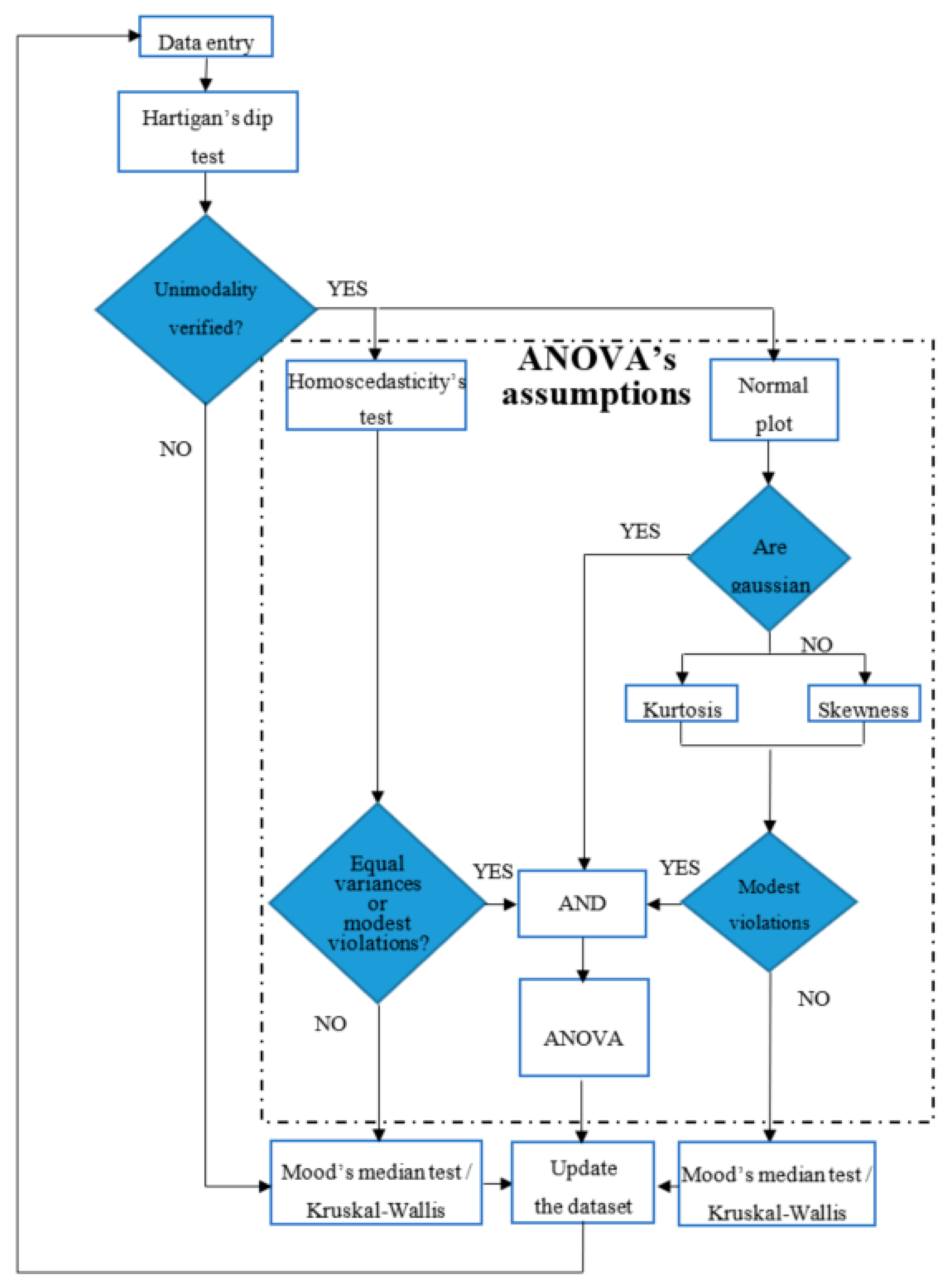
The columns of the matrix (1) are independent each other, because the values of each array are acquired by devoted acquisition units, so no inter-dependence exists among the values of the columns, which can be considered as separate statistical populations. The flow chart in Figure 1 proposes a methodology to verify the energy performance of a PV plant and to detect and locate any anomaly before it becomes a failure. The methodology is particularly useful when the PV plant is not equipped with weather station, because, in this case, the evaluations about the energy performance cannot be carried out with respect to the solar radiation, cell temperature, and so on.
The absence of the weather station is very frequent for PV systems with nominal peak power up to 100 kWp. So, the proposed methodology allows for supervising the energy performance of a PV plant on the basis of a mutual comparison among its arrays, with no environmental data as input. Obviously, this approach is valid, only if the arrays are identical (same PV modules, same number of modules, same slope, same tilt, same inverters, and so on); in fact, under this assumption, the energy productions of the arrays must be almost identical in each period and in the whole year (the changing environmental conditions affect the arrays in the same way, if they are installed next to each other). So, the comparative and cumulative monitoring of the energy performance of identical arrays allows to declare, within the uncertainty defined by the value of the significance level α, if the arrays are producing the same energy or not. This goal can be pursued by using the parametric tests or the non-parametric tests. Since the parametric tests are based on known distribution, they are more reliable than the non-parametric ones, which are, instead, distribution-free. For this reason, it is advisable to use always the parametric tests, provided that all of the needed constraints are satisfied. In particular, the parametric test known as ANalysis Of VAriance (ANOVA) [21] compares the variance inside each array distribution and the variance among the arrays’ distributions. In other words, ANOVA evaluates whether the differences of the mean values of the different groups are statistically significant or not. ANOVA is based on the null hypothesis H0 (Equation (2)) that the means of the distributions, , are equal:
versus the alternative hypothesis that the mean value of at least one distribution is different from the others. In rigorous way, ANOVA can be used under the assumptions:
- (a)
- all the observations are mutually independent;
- (b)
- all the distributions have equal variance; and,
- (c)
- all the distributions are normally distributed.
Nevertheless, ANOVA can be applied also for limited violations of the assumptions (b) and (c), whereas the assumption (a) is always verified, if the measures come from independent local measurement units.
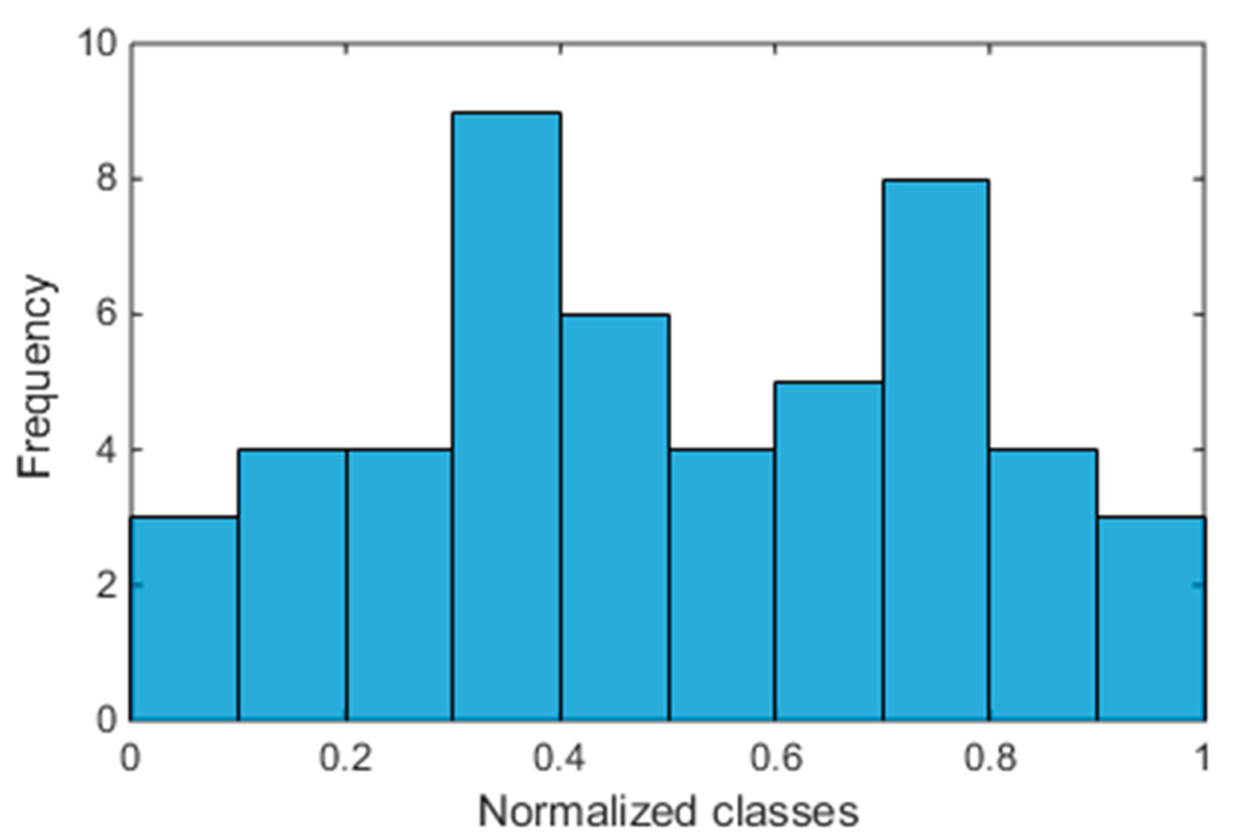
So, before applying ANOVA test, several verifications are needed and they are the blue blocks of Figure 1. The first check regards the unimodality of the dataset of each array, because a multimodality distribution, e.g., the bimodal distribution in Figure 2, is surely non-normal. The Hartigan’s Dip Test (HDT) is able to check the unimodality [22] and is based on the null hypothesis that the distribution is unimodal versus the alternative one that it is at least bi-modal.
Usually, the test hypothesis is defined with the significance value α = 0.05; so, if p-value , then the null hypothesis is rejected, when considering it as acceptable to have a 5% probability of incorrectly rejecting the null hypothesis. This is known as type I error. Smaller values of α are not advisable to study the data of a medium-large PV plant, because the higher complexity of the whole system requires a larger uncertainty to be accepted. The verification of the unimodality can be also done on the basis of a relationship between the values of skewness and kurtosis [23,24]; nevertheless, in this paper only HDT will be used, because it is usually more sensitive than other methods.
If the unimodality check is not passed, the distribution is not gaussian and ANOVA cannot be used, then a nonparametric test has to be applied. In the general case of N arrays, with , the nonparametric test to be used has to be chosen between Kruskal-Wallis test (K-W) [25,26] and Mood’s Median test (MM), which do not require that the distributions are gaussian, but only that the distributions are continuous. In presence of outliers, MM performs better than K-W.
Instead, if the unimodality is satisfied, other checks are needed, before deciding whether ANOVA can be applied. First of all, it is needed to verify the previous assumptions (b) and (c). If both of them are satisfied, ANOVA can be applied. Otherwise, since ANOVA is effective also for modest violations of those assumptions, then it is needed to quantify the entity of the violations. With this in mind, the condition (b) on the variance can be verified by means of the Homoscedasticity’s Test (HT), which is again a hypothesis test that returns a p-value. So, also in this case, it is possible to fix the significance value α = 0.05 (accepting the 5% of probability of type I error) and to compare it with the p-value. If the inequality p-value is satisfied, the variances of the distributions of the arrays are different, thus, the condition (b) is violated, and ANOVA cannot be applied. In this case, it is necessary to use K-W or MM, depending on the presence or absence of the outliers. Otherwise, ANOVA could be applied, if even the condition (c) is satisfied, eventually with a modest violation. To check the condition (c), an effective tool is the normal probability plot [27], which returns information about the range of percentiles that fall into the normal distribution. If the feedback from the normal plot is not exhaustive to decide if the condition (c) is satisfied, then it needs to calculate the values of skewness (Equation (3)) and kurtosis (Equation (4)) of each distribution [19]. Skewness, , is defined as:
where µ is the mean of the data x, σ is the standard deviation of x, and E(t) represents the expected value of the quantity t. The skewness is the third standardized moment and measures the asymmetry of the data around the mean value. Only for the distribution is symmetric; this is a necessary, but not sufficient condition for a gaussian distribution. In fact, while the gaussian distribution is surely symmetric, nevertheless there exist also symmetric but not gaussian distributions. Therefore, the only value of the skewness is not exhaustive. For this reason, it is needed to calculate also the kurtosis, , here defined as the Pearson’s kurtosis less 3 (also known as excess kurtosis) and calculated as:
The kurtosis is the fourth standardized moment and measures the tailedness of the distribution. Only for , the distribution is mesokurtic, which is the necessary but not sufficient condition for a gaussian distribution. Other details can be found in [19]. The set of the two indices (skewness and kurtosis) allows for quantifying the mismatch of the distribution with respect to a gaussian one and to evaluate if the violation of the condition (c) is acceptable or not, even if the maximum acceptable mismatches are not unique [28,29,30]. Only if also this verification is passed, the ANOVA test can be applied; otherwise a non-parametric test has to be used.
As new data are acquired and the size of the energy dataset increases, the monitoring becomes more accurate, allowing for the estimation and location also of a low-intensity anomaly, before it becomes a fault.
3. Description of the PV Plant under Investigation
The energy performance of a real operating 90 kWp grid-connected PV plant, installed in a private area of a company located in Bari, a city in the south of Italy, has been studied. It injects the energy exceeding the local consumptions into the distribution network. The 600 modules of the PV plant are equally divided in six arrays. The nominal power of a single module is 150 Wp (Sol 150, mono-crystalline, by Solterra), whereas the nominal peak power for a single array is 15,000 Wp. Each array is connected to a 15 kW inverter (Sunny Tripower 15000TL by SMA, Milan, Italy). The plant has an interface device, able to automatically connect itself to the grid. The system faces the south and is sloped at about 35°. By inserting these values in the well-known PhotoVoltaic Geographical Information System (PVGIS) [31] of the European Commission Joint Research Centre (EC-JRC), and based on the historical data of the solar irradiance, it results that the estimated yearly energy production is about 117,680 kWh, corresponding to about 1307 kWh/kWp per year. Moreover, the website provides also the estimated monthly energy production, which will be used in the next Section 4.1, Section 4.2 and Section 4.3.
The PV plant is equipped with a datalogger that acquires data from the six arrays. The datalogger has a sample time of 2 s, while internal software calculates the mean of all the measures after 10 min and only this last value is stored into a database. The monitoring system measures and stores the values of total power and energy on the AC side of each inverter, the number of the operating hours, and the voltage VDC on the DC side of each inverter. The capacity of the monitoring equipment is up one year. The observation period refers to a full year during which the PV plant has shown some malfunctions, whereas in the previous years the PV plant has not shown any malfunction, therefore the results of the previous year are not reported in the paper.
4. Cumulative Statistical Analysis
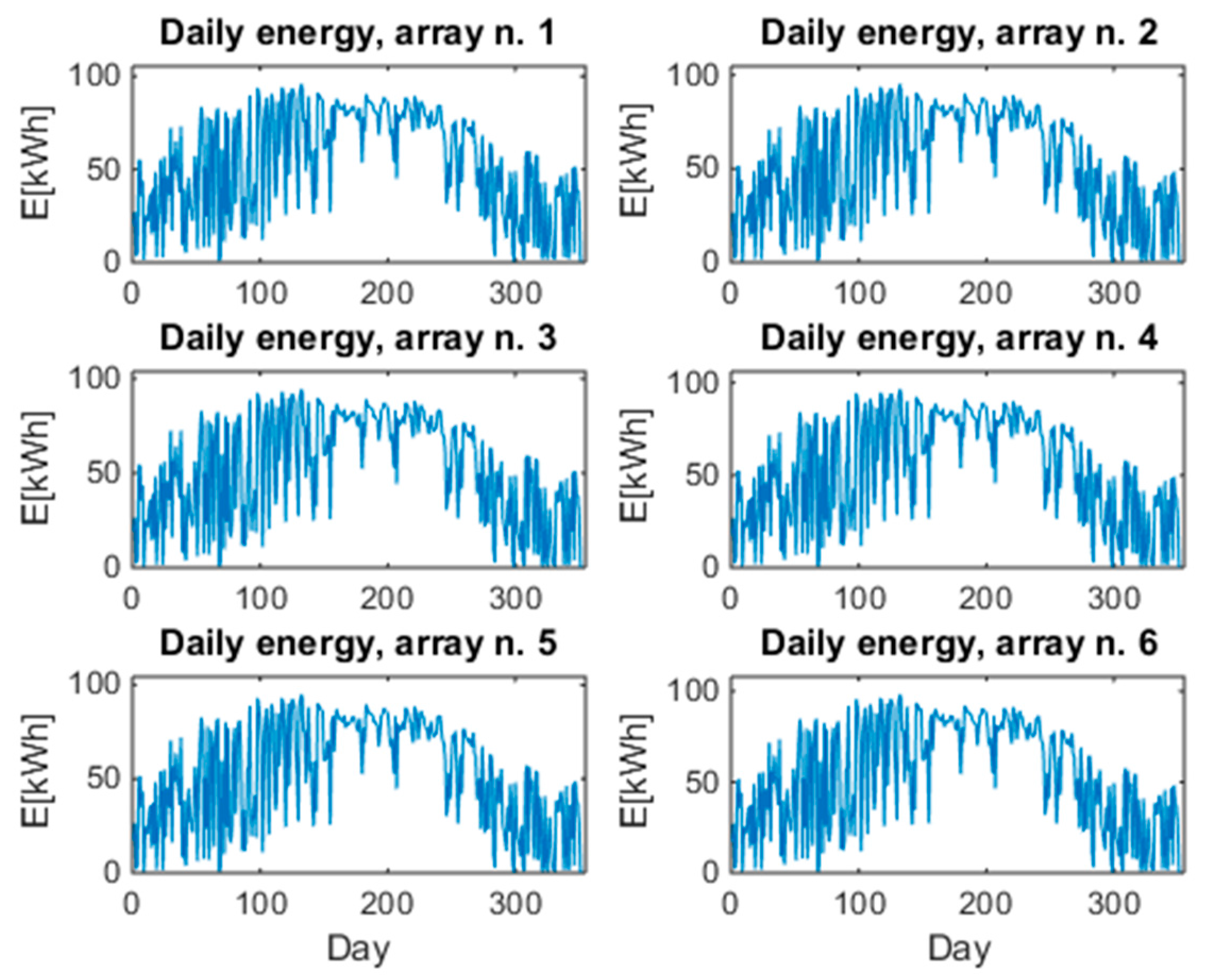
The energy performance of the PV plant described in Section 3 has been studied by means of the statistical methodology proposed in Section 2. Statistical data analysis has been carried out in Matlab R2017 environment by using the standard routines of the Statistics toolbox and by implementing the flow chart of Figure 1. Figure 3 diagrams the daily energy that is produced by each array during a whole year and it seems that no anomaly is present. In fact, the diagrams seem to be superimposable.
Three analyses are discussed to evaluate the trends of the energy performances of the PV plant. The increase of the time window described in Figure 1 allows for understanding how some characteristic benchmarks of the PV plants vary during the year as the new data are acquired. The trend of the parameters can be very useful to detect and locate possible low-intensity anomalies. Following results will be discussed:
- one-month analysis (January);
- six-months analysis (January–June); and,
- one-year analysis (January–December).
The following results will be reported for each analysis: p-value of the HDT for each array, p-value of the HT, normal probability plot, box plot of the ANOVA or K-W test, mean, median, variance, and relative spreads of each one of them, skewness and kurtosis, p-value for ANOVA, or K-W test.
4.1. One-Month Analysis (January)
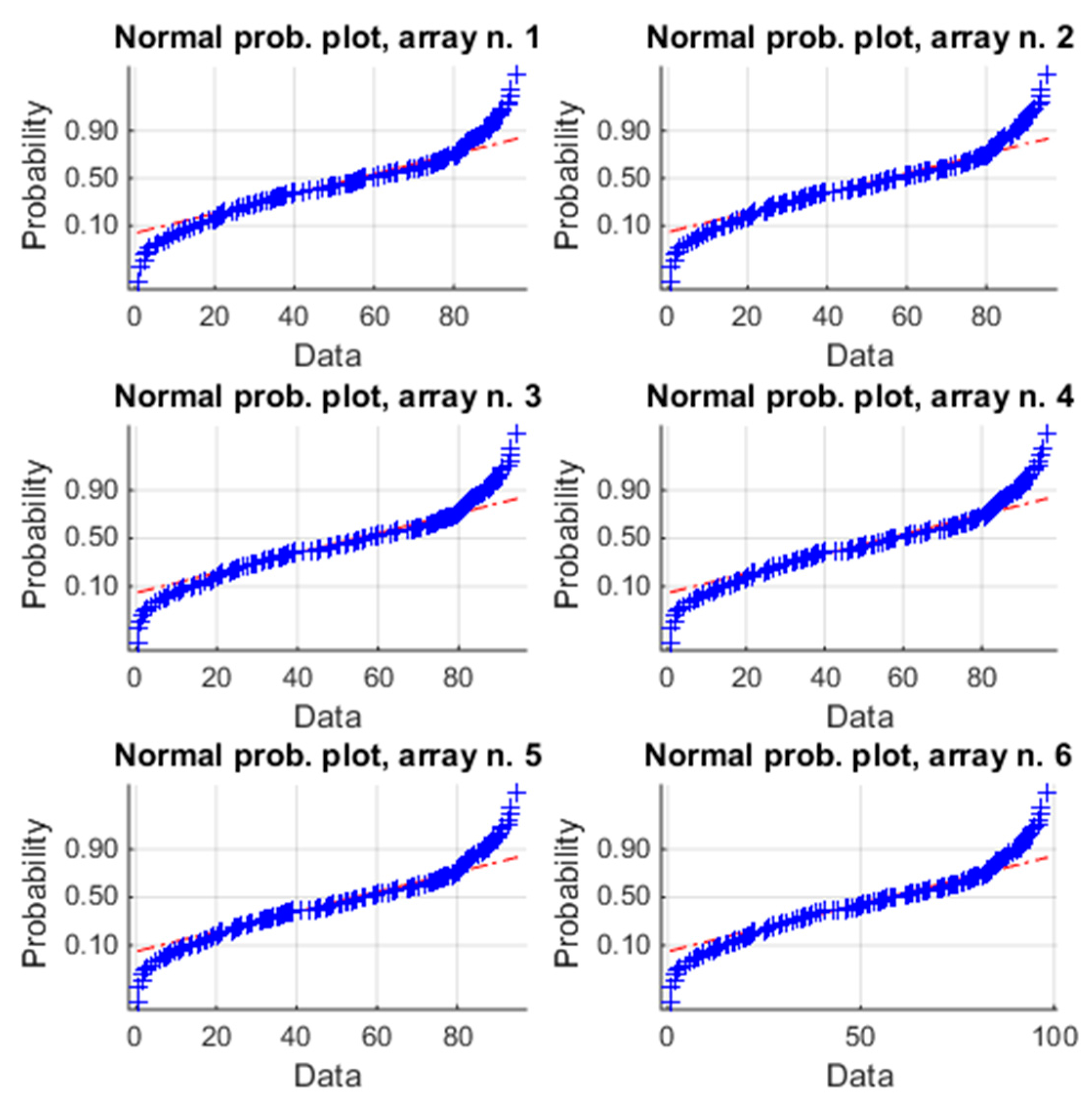
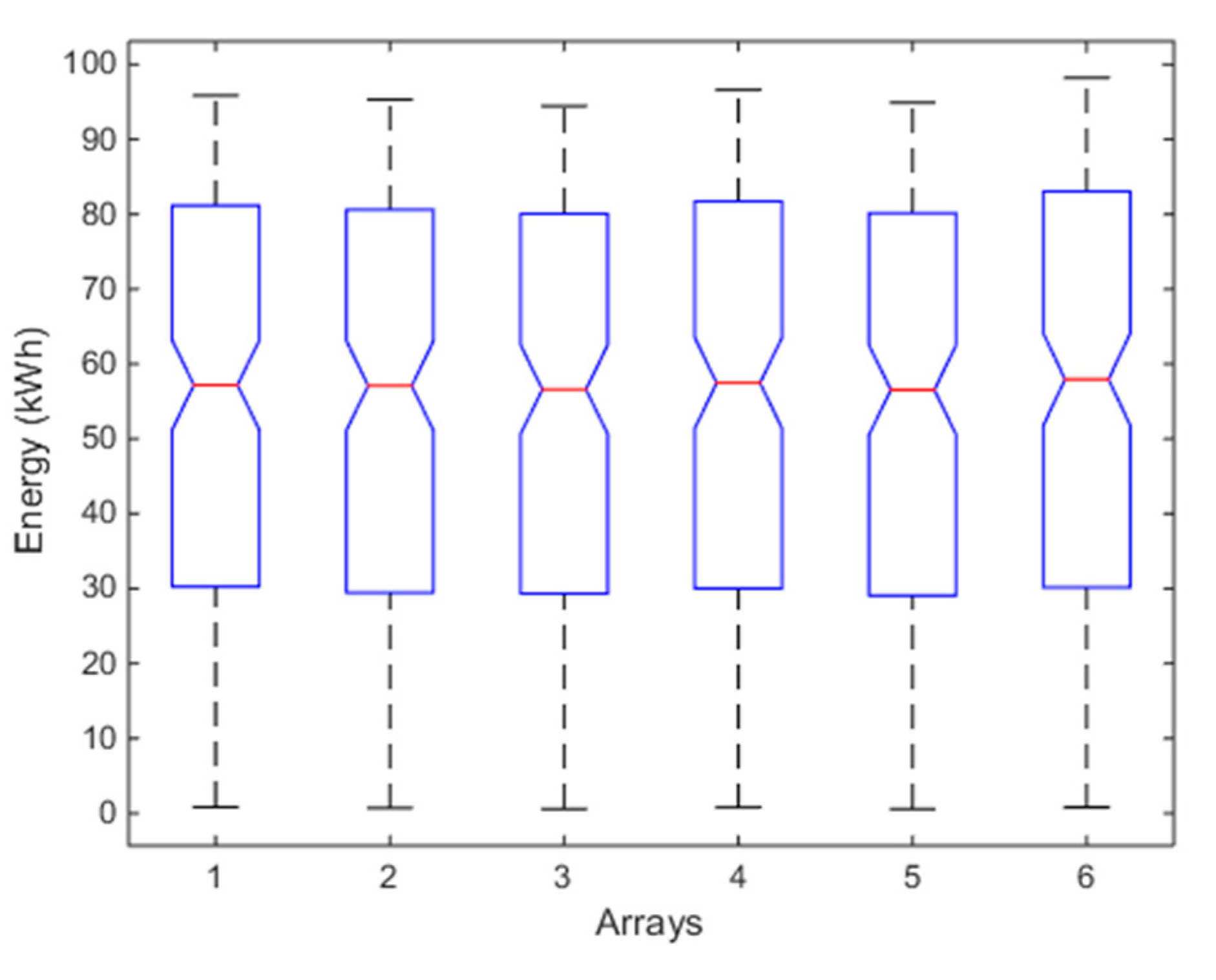
Table 1 reports the p-value of HDT for each array, the p-value of HT, the means, medians, and variances of the energy produced by each array, the global means of them and the spreads in per cent. With respect to the unimodality condition (first blue block of Figure 1), the p-value of HDT is calculated for each array and it is higher than α = 0.05, so all the distributions are unimodal. To apply ANOVA, conditions (b) and (c) have to be verified. The p-value = 1 of HT in Table 1 (again higher than α = 0.05) says that the homoscedasticity is verified, thus also the condition (b) is verified. In order to verify the condition (c), the normal probability plot (Figure 4) is used. Since almost all the data of each array belong to the straight red line, the distributions are gaussian. Therefore, the main conditions of the flow chart in Figure 1 are satisfied and ANOVA can be applied. The box plots of Figure 5 highlight that the six arrays produce almost the same energy, either with respect to the median value (in red color), or either with respect to the first and third inter-quartiles; moreover, outliers are absent. Therefore, the energy performances of the arrays are similar and no anomaly is present in the PV plants. These considerations are also supported by the values of means, medians and spreads in Table 1. Particularly, from [31], it results that the estimated average energy of the PV plant in January should be about 5770 kWh, corresponding to a daily average energy for each array of about 5770/(31 × 6) = 31.0 kWh, that is almost equal to the global mean value 30.19 kWh of Table 1. Moreover, the well working of the whole PV plant is also confirmed by the highest p-value of ANOVA (0.999) that is reported in the Table 2, which also collects the values of skewness and kurtosis for each array. Even if they are not necessary in this case, because the normal probability plot has not evidenced a violation of condition (c), nevertheless it is useful to calculate these indices at each step, in order to follow their trends.
4.2. Six-Months Analysis (January–June)
In this analysis, the data of the previous analysis and the successive five months are included. Table 3 reports the analogous values of Table 1. Also, in this case, the unimodality is satisfied for each array (p-values of HDT), as well as the homoscedasticity (p-value of HT). Instead, Figure 6 reports the normal probability plot and it is evident that the data belong to the red line only in the range [0.2~0.6], thus the distributions are not gaussian and it is needed to evaluate the violation of the condition c) by means of skewness and kurtosis (Table 4). Now, both of the indices of each array are different from zero, but the absolute values of kurtosis are also higher than 1, which is largely considered as the maximum acceptable threshold to consider the violation modest. As already said in the Introduction, there is not an unambiguous position on this point. Moreover, all of the values of skewness have changed sign, becoming negative; this means that the asymmetry of the distribution of each array is changed during the six months under investigation. Therefore, the violation of the condition (c) is not negligible and flow chart of Figure 1 suggests to avoid ANOVA and to apply a non-parametric test. The box plot of Figure 7, based on K-W, confirms again that the arrays have similar energy productions (see also the p-value in Table 4). Particularly, from [31], it results that the estimated average energy of the PV plant in the period January-June should be about 58,700 kWh, corresponding to a daily average energy for each array of about 58,700/(181 × 6) = 54.05 kWh, that is almost equal to the global mean value 54.41 kWh of Table 3. The box plot of the array n. 6 is slightly different from the others. This is confirmed also by observing the spreads of the means and of the medians in Table 3, as well as the values of the skewness (array n. 6 has the maximum values).
4.3. One-Year Analysis (January–December)
From Table 5, it results that the unimodality is satisfied for each array (p-values of HDT), even if the p-value of the array n. 6 is quite different from the other ones. The homoscedasticity (p-value of HT) is also satisfied. Figure 8 diagrams the normal probability plot of each distribution and the data belong to the red line only in the range [0.2~0.6], thus the distributions are not gaussian and it is needed to evaluate the violation of the condition (c) by means of skewness and kurtosis (Table 6). Now, both the indices of each array are different from zero and the absolute values of kurtosis are higher than 1. Both of the indices confirm the sign of the previous analysis. The violation of the condition (c) is not negligible and flow chart of Figure 1 suggests using a non-parametric test. The box plot of Figure 9, based on K-W, confirms again that the arrays have similar energy productions. Particularly, from [31], it results that the estimated average energy of the PV plant in the period January–December should be about 117,680 kWh, corresponding to a daily average energy for each array of about 117,680/(365 × 6) = 53.73 kWh, that is almost equal to the global mean value 53.46 kWh of Table 5. The box plot of the array n. 6 is again slightly different from the others. Moreover, the p-value in Table 6 is less than the p-value of the previous analysis. By observing the spreads of the means in Table 5 and the skewness in Table 6, array n. 6 shows a slightly different energy performance, which represents an alert about the presence of a low-intensity anomaly.
4.4. Discussion
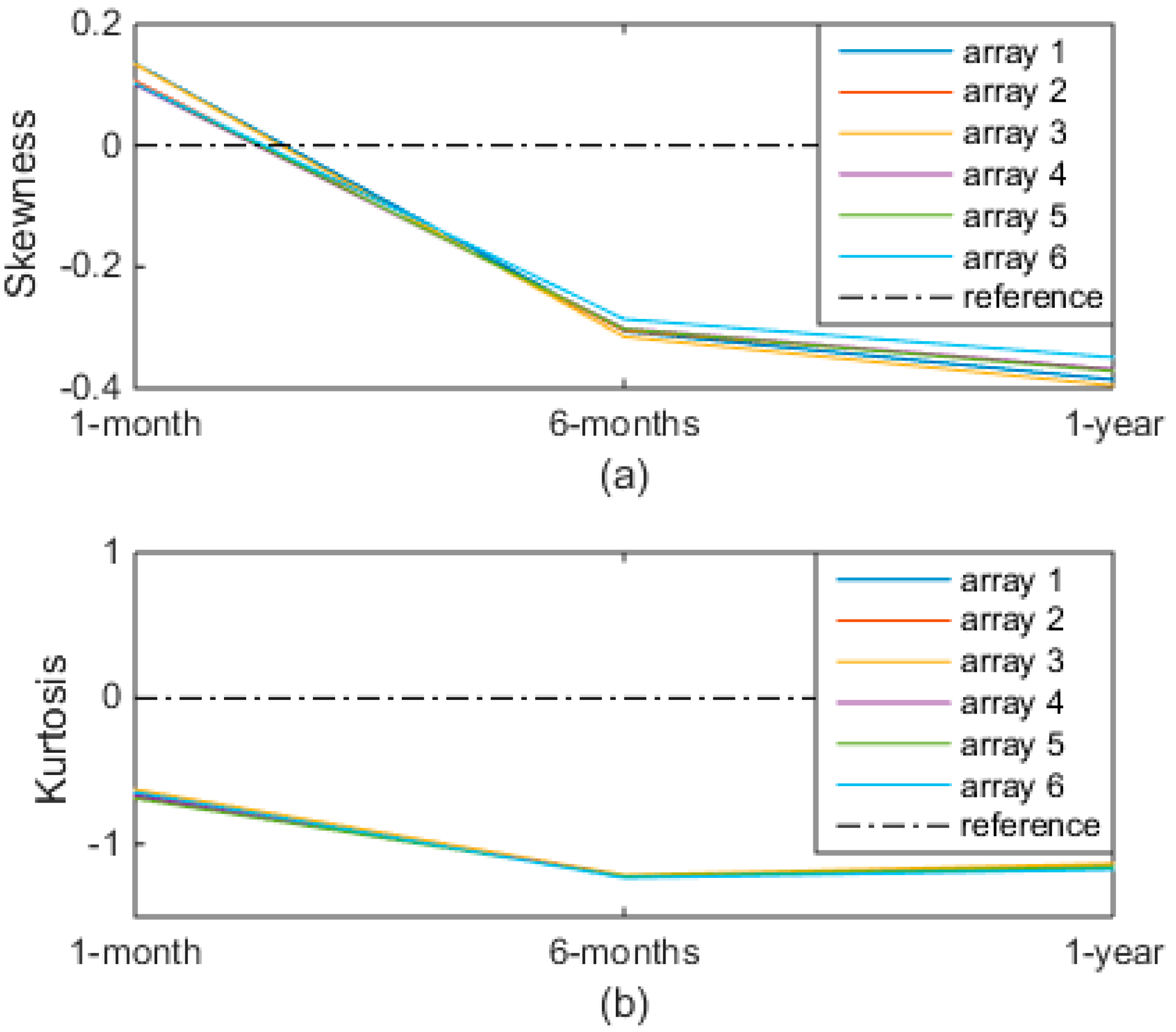
As the real operating PV systems are affected by the atmospheric phenomena, their energy distributions are never gaussian, as shown in the previous analyses. Then, the parametric tests should never been applied. Instead, since ANOVA can be applied for modest violations of its assumptions, the issue consists in quantifying the violation, in order to decide whether it is negligible or not. Moreover, the previous analyses have also shown that it is not sufficient for only one parameter to state whether the violation is modest or not. In fact, Figure 10 groups the values of both skewness and kurtosis reported in the Table 2, Table 4 and Table 6. It results that: (a) the values of skewness are always near the zero, but they change the sign, meaning that the asymmetry changes during the year; (b) the values of kurtosis are always negative, but they exceeds the value −1 (that is considered the maximum acceptable violation by several researchers) in both the second and third analyses. Therefore, if only skewness had been calculated, the violation would have always been limited and ANOVA would have always been used. Instead, the values of kurtosis have suggested using ANOVA only in the first analysis and not in the other two analyses. The issue of the quantification of the violation of the ANOVA’s assumptions is still open and is a very interesting topic for a future work.
5. Conclusions
The paper proposes a procedure to statistically analyze the PV plant operation without the environmental data as input. The procedure is cumulative and some benchmarks are calculated as new data are acquired. The real case study shows three analyses to explain how the procedure is applied during a complete year, but it can be also used for a real-time monitoring, after specific performance benchmarks have been fixed. In this way, it is possible to follow the trend of the benchmarks and to detect and locate the low-intensity anomalies, before they become failures. Obviously, the number of applications of cumulative analysis for detecting an anomaly depends on its severity. A real case study has shown the effectiveness of the proposed approach in detecting a low-intensity anomaly in the array n. 6. In fact, the proposed procedure has allowed revealing an anomaly that had not been detected, by using the standard indexes. The procedure does not allow identifying the cause of the anomaly, but only to detect and locate it. Finally, ANOVA can be applied also for modest violations of the assumptions, even if nowadays there is not a fixed procedure to evaluate the amount of the violations, and, consequently, to decide whether the violations are negligible or not. The proposed algorithm is a useful start point to investigate in depth the new approaches to establish which are the thresholds for modest violations. The proposed approach is particularly effective for PV plants that are not equipped with a weather station, as it often happens for small-medium size PV plants. The industrial community can use the proposed algorithm to monitor several PV plants with different characteristics, in order to classify the different low-intensity anomalies and to improve the energy performance of the PV plants. In general, these anomalies can depend on the premature ageing, on the production process of the components, on the design of the PV plants, on the installation stage, and so on. The proposed algorithm can be a valid support for the classification of the anomalies and then for the predictive maintenance.
Conflicts of Interest
The author declares no conflict of interest.
References
- Grimaccia, F.; Leva, S.; Mussetta, M.; Ogliari, E. ANN sizing procedure for the day-ahead output power forecast of a PV plant. Appl. Sci. 2017, 7, 622. [Google Scholar] [CrossRef]
- Massi Pavan, A.; Vergura, S.; Mellit, A.; Lughi, V. Explicit empirical model for photovoltaic devices. Experimental validation. Sol. Energy 2017, 155, 647–653. [Google Scholar] [CrossRef]
- Dellino, G.; Laudadio, T.; Mari, R.; Mastronardi, N.; Meloni, C.; Vergura, S. Energy Production Forecasting in a PV Plant Using Transfer Function Models. In Proceedings of the 2015 IEEE 15th International Conference on Environment and Electrical Engineering (EEEIC), Rome, Italy, 10–13 June 2015. [Google Scholar]
- Guerriero, P.; Di Napoli, F.; Vallone, G.; D’Alessandro, V.; Daliento, S. Monitoring and diagnostics of PV plants by a wireless self-powered sensor for individual panels. IEEE J. Photovolt. 2015, 6, 286–294. [Google Scholar] [CrossRef]
- Johnston, S.; Guthrey, H.; Yan, F.; Zaunbrecher, K.; Al-Jassim, M.; Rakotoniaina, P.; Kaes, M. Correlating multicrystalline silicon defect types using photoluminescence, defect-band emission, and lock-in thermography imaging techniques. IEEE J. Photovolt. 2014, 4, 348–354. [Google Scholar] [CrossRef]
- Peloso, M.; Meng, L.; Bhatia, C.S. Combined thermography and luminescence imaging to characterize the spatial performance of multicrystalline Si wafer solar cells. IEEE J. Photovolt. 2015, 5, 102–111. [Google Scholar] [CrossRef]
- Vergura, S.; Marino, F. Quantitative and computer aided thermography-based diagnostics for PV devices: Part I—Framework. IEEE J. Photovolt. 2017, 7, 822–827. [Google Scholar] [CrossRef]
- Vergura, S.; Colaprico, M.; de Ruvo, M.F.; Marino, F. A quantitative and computer aided thermography-based diagnostics for PV devices: Part II—Platform and results. IEEE J. Photovolt. 2017, 7, 237–243. [Google Scholar] [CrossRef]
- Mekki, H.; Mellit, A.; Salhi, H. Artificial neural network-based modelling and fault detection of partial shaded photovoltaic modules. Simul. Model. Pract. Theory 2016, 67, 1–13. [Google Scholar] [CrossRef]
- Vergura, S. Scalable Model of PV Cell in Variable Environment Condition Based on the Manufacturer Datasheet for Circuit Simulation. In Proceedings of the 2015 IEEE 15th International Conference on Environment and Electrical Engineering (EEEIC), Rome, Italy, 10–13 June 2015. [Google Scholar]
- Harrou, F.; Sun, Y.; Kara, K.; Chouder, A.; Silvestre, S.; Garoudja, E. Statistical fault detection in photovoltaic systems. Sol. Energy 2017, 150, 485–499. [Google Scholar]
- Vergura, S.; Carpentieri, M. Statistics to detect low-intensity anomalies in PV systems. Energies 2018, 11, 30. [Google Scholar] [CrossRef]
- Ventura, C.; Tina, G.M. Development of models for on line diagnostic and energy assessment analysis of PV power plants: The study case of 1 MW Sicilian PV plant. Energy Procedia 2015, 83, 248–257. [Google Scholar] [CrossRef]
- Il-Song, K. On-line fault detection algorithm of a photovoltaic system using wavelet transform. Sol. Energy 2016, 226, 137–145. [Google Scholar]
- Rabhia, A.; El hajjajia, A.; Tinab, M.H.; Alia, G.M. Real time fault detection in photovoltaic systems. Energy Procedia 2017, 11, 914–923. [Google Scholar]
- Plato, R.; Martel, J.; Woodruff, N.; Chau, T.Y. Online fault detection in PV systems. IEEE Trans. Sustain. Energy 2015, 6, 1200–1207. [Google Scholar] [CrossRef]
- Ando, B.; Bagalio, A.; Pistorio, A. Sentinella: Smart monitoring of photovoltaic systems at panel level. IEEE Trans. Instrum. Meas. 2015, 64, 2188–2199. [Google Scholar] [CrossRef]
- IEC International Standard 61724—Photovoltaic System Performance Monitoring—Guidelines for Measurement, Data Exchange and Analysis; International Electrotechnical Commission: Geneva, Switzerland, 1998.
- Leloux, J.; Narvarte, L.; Trebosc, D. Review of the performance of residential PV systems in Belgium. Renew. Sustain. Energy Rev. 2012, 16, 178–184. [Google Scholar] [CrossRef] [Green Version]
- Leloux, J.; Narvarte, L.; Trebosc, D. Review of the performance of residential PV systems in France. Renew. Sustain. Energy Rev. 2012, 16, 1369–1376. [Google Scholar] [CrossRef] [Green Version]
- Hogg, R.V.; Ledolter, J. Engineering Statistics; MacMillan: Basingstoke, UK, 1987. [Google Scholar]
- Hartigan, J.A.; Hartigan, P.M. The dip test of unimodality. Ann. Stat. 1985, 13, 70–84. [Google Scholar] [CrossRef]
- Rohatgi, V.K.; Szekely, G.J. Sharp inequalities between skewness and kurtosis. Stat. Probab. Lett. 1989, 8, 297–299. [Google Scholar] [CrossRef]
- Klaassen, C.A.J.; Mokveld, P.J.; van Es, B. Squared skewness minus kurtosis bounded by 186/125 for unimodal distributions. Stat. Probab. Lett. 2000, 50, 131–135. [Google Scholar] [CrossRef]
- Gibbons, J.D. Nonparametric Statistical Inference, 2nd ed.; M. Dekker: New York, NY, USA, 1985. [Google Scholar]
- Hollander, M.; Wolfe, D.A. Nonparametric Statistical Methods; Wiley: Hoboken, NJ, USA, 1973. [Google Scholar]
- Chambers, J.; Cleveland, W.; Kleiner, B.; Tukey, P. Graphical Methods for Data Analysis; Wadsworth: Belmont, CA, USA, 1983. [Google Scholar]
- Gravetter, F.; Wallnau, L. Essentials of Statistics for the Behavioral Sciences, 8th ed.; Wadsworth: Belmont, CA, USA, 2014. [Google Scholar]
- Tabachnick, B.G.; Fidell, L.S. Using Multivariate Statistics, 6th ed.; Pearson: London, UK, 2013. [Google Scholar]
- George, D.; Mallery, P. SPSS for Windows Step by Step. A Simple Guide and Reference 17.0 Update, 10th ed.; Pearson: Boston, MA, USA, 2010. [Google Scholar]
- PVGIS. Available online: http://re.jrc.ec.europa.eu/pvg_tools/en/tools.html (accessed on 25 February 2018).
Figure 1.
Statistical methodology.

Figure 2.
Example of histogram of a bimodal distribution.

Figure 3.
Daily energy produced by each array during the whole year.

Figure 4.
Normal plot of the energy of the six arrays for one-month analysis. The blue symbols “+” are the samples; the red line is the reference for a normal distribution.
Figure 4.
Normal plot of the energy of the six arrays for one-month analysis. The blue symbols “+” are the samples; the red line is the reference for a normal distribution.

Figure 5.
Box plot of ANOVA test of the six arrays for the one-month analysis. For each box, the red mark represents the median, and the bottom and top edges of the box indicate the 25th and 75th percentiles, respectively. The whiskers are to the most extreme elements.
Figure 5.
Box plot of ANOVA test of the six arrays for the one-month analysis. For each box, the red mark represents the median, and the bottom and top edges of the box indicate the 25th and 75th percentiles, respectively. The whiskers are to the most extreme elements.
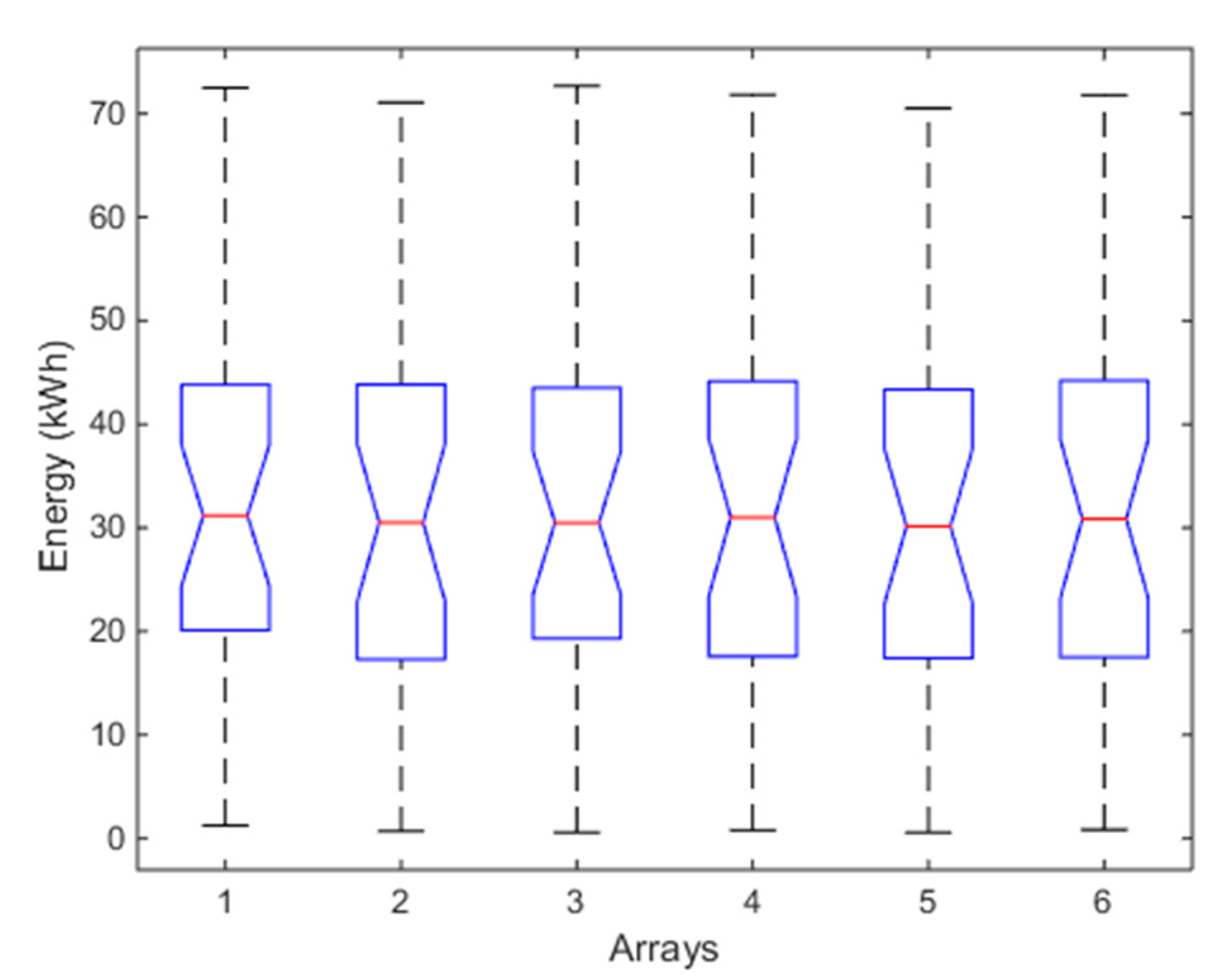
Figure 6.
Normal plot of the energy of the six arrays for the six-month analysis. The blue symbols “+” are the samples; the red line is the reference for a normal distribution.
Figure 6.
Normal plot of the energy of the six arrays for the six-month analysis. The blue symbols “+” are the samples; the red line is the reference for a normal distribution.

Figure 7.
Box plot of K-W test of the six arrays for the six-month analysis. For each box, the red mark represents the median, and the bottom and top edges of the box indicate the 25th and 75th percentiles, respectively. The whiskers are to the most extreme elements.
Figure 7.
Box plot of K-W test of the six arrays for the six-month analysis. For each box, the red mark represents the median, and the bottom and top edges of the box indicate the 25th and 75th percentiles, respectively. The whiskers are to the most extreme elements.

Figure 8.
Normal plot of the energy of the six arrays for the one-year analysis. The blue symbols “+” are the samples; the red line is the reference for a normal distribution.
Figure 8.
Normal plot of the energy of the six arrays for the one-year analysis. The blue symbols “+” are the samples; the red line is the reference for a normal distribution.
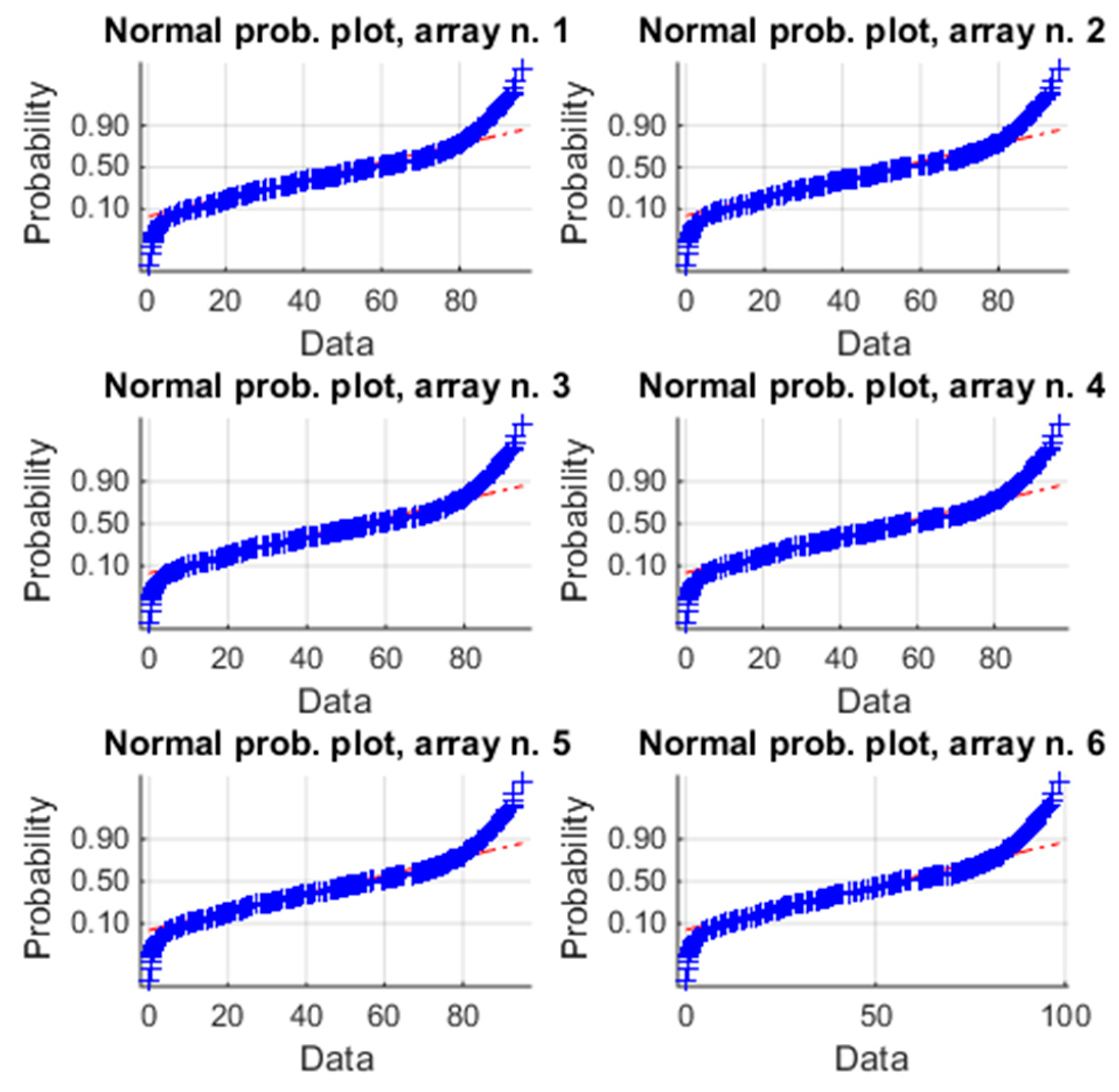
Figure 9.
Box plot of K-W test of the six arrays for the one-year analysis. For each box, the red mark represents the median, and the bottom and top edges of the box indicate the 25th and 75th percentiles, respectively. The whiskers are to the most extreme elements.
Figure 9.
Box plot of K-W test of the six arrays for the one-year analysis. For each box, the red mark represents the median, and the bottom and top edges of the box indicate the 25th and 75th percentiles, respectively. The whiskers are to the most extreme elements.
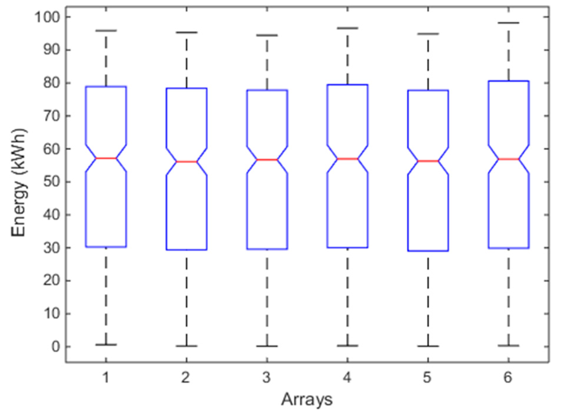
Figure 10.
Trend of skewness and kurtosis of the six arrays.


Table 1.
p-Value of Hartigan’s Dip Test (HDT) and Homoscedasticity’s Test (HT); daily mean, median and variance of the energy (in kWh) produced by each array and spread with respect to the global values for one month.
Table 1.
p-Value of Hartigan’s Dip Test (HDT) and Homoscedasticity’s Test (HT); daily mean, median and variance of the energy (in kWh) produced by each array and spread with respect to the global values for one month.
| Array Number | ||||||
|---|---|---|---|---|---|---|
| Parameter | 1 | 2 | 3 | 4 | 5 | 6 |
| p-value (HDT) | 0.534 | 0.678 | 0.418 | 0.624 | 0.624 | 0.648 |
| p-value (HT) | 1 | |||||
| Mean | 30.90 | 29.81 | 30.31 | 30.30 | 29.63 | 30.19 |
| Global mean | 30.19 | |||||
| Spread % | 2.35 | −1.24 | 0.41 | 0.35 | −1.85 | 0.00 |
| Median | 31.19 | 30.50 | 30.46 | 31.00 | 30.14 | 30.86 |
| Global mean | 30.69 | |||||
| Spread % | 1.61 | −0.63 | −0.71 | 1.00 | −1.80 | 0.53 |
| Variance | 344.2 | 337.7 | 351.7 | 343.0 | 336.2 | 339.0 |
| Global mean | 342.0 | |||||
| Spread % | 0.66 | −1.25 | 2.84 | 0.31 | −1.70 | −0.87 |
Table 2.
p-Value of ANOVA, skewness and kurtosis for the arrays (1~6), (1-month).
| Array Number | ||||||
|---|---|---|---|---|---|---|
| Parameter | 1 | 2 | 3 | 4 | 5 | 6 |
| 0.135 | 0.107 | 0.134 | 0.100 | 0.103 | 0.103 | |
| −0.65 | −0.68 | −0.63 | −0.67 | −0.69 | −0.64 | |
| p-value (ANOVA) | 0.999 | |||||
Table 3.
p-value of HDT and HT; daily mean, median and variance of the energy (in kWh) produced by each array and spread with respect to the global values for 6 months.
Table 3.
p-value of HDT and HT; daily mean, median and variance of the energy (in kWh) produced by each array and spread with respect to the global values for 6 months.
| Array Number | ||||||
|---|---|---|---|---|---|---|
| Parameter | 1 | 2 | 3 | 4 | 5 | 6 |
| p-value(HDT) | 0.784 | 0.838 | 0.720 | 0.808 | 0.806 | 0.862 |
| p-value(HT) | 0.984 | |||||
| Mean | 54.72 | 54.02 | 53.67 | 54.90 | 53.61 | 55.58 |
| Global mean | 54.41 | |||||
| Spread % | 0.57 | −0.73 | −1.36 | 0.89 | −1.48 | 2.10 |
| Median | 57.19 | 57.09 | 56.60 | 57.46 | 56.54 | 57.95 |
| Global mean | 57.14 | |||||
| Spread % | 0.08 | −0.08 | −0.94 | 0.56 | −1.05 | 1.42 |
| Variance | 770.6 | 775.2 | 764.6 | 796.6 | 770.0 | 822.9 |
| Global mean | 783.3 | |||||
| Spread % | −1.62 | −1.04 | −2.39 | 1.69 | −1.70 | 5.05 |
Table 4.
p-value of K-W, skewness and kurtosis for the arrays (1~6), (6-months).
| Array Number | ||||||
|---|---|---|---|---|---|---|
| Parameter | 1 | 2 | 3 | 4 | 5 | 6 |
| −0.31 | −0.30 | −0.31 | −0.3 | −0.30 | −0.28 | |
| −1.22 | −1.22 | −1.21 | −1.22 | −1.22 | −1.22 | |
| p-value (K-W) | 0.927 | |||||
Table 5.
p-Value of HDT and HT; daily mean, median and variance of the energy (in kWh) produced by each array and spread with respect to the global values for 1 year.
Table 5.
p-Value of HDT and HT; daily mean, median and variance of the energy (in kWh) produced by each array and spread with respect to the global values for 1 year.
| Array Number | ||||||
|---|---|---|---|---|---|---|
| Parameter | 1 | 2 | 3 | 4 | 5 | 6 |
| p-value(HDT) | 0.916 | 0.866 | 0.816 | 0.876 | 0.874 | 0.632 |
| p-value(HT) | 0.926 | |||||
| Mean | 53.84 | 53.05 | 52.87 | 53.88 | 52.68 | 54.46 |
| Global mean | 53.46 | |||||
| Spread % | 0.71 | −0.77 | −1.12 | 0.78 | −1.46 | 1.87 |
| Median | 57.16 | 56.13 | 56.70 | 56.96 | 56.29 | 56.90 |
| Global mean | 56.69 | |||||
| Spread % | 0.83 | −0.99 | 0.02 | 0.48 | −0.71 | 0.38 |
| Variance | 771.6 | 778.3 | 764.9 | 797.8 | 771.0 | 824.5 |
| Global mean | 784.7 | |||||
| Spread % | −1.67 | −0.81 | −2.51 | 1.67 | −1.75 | 5.08 |
Table 6.
p-Value of K-W, skewness and kurtosis for the arrays (1~6), (1-year).
| Array Number | ||||||
|---|---|---|---|---|---|---|
| Parameter | 1 | 2 | 3 | 4 | 5 | 6 |
| −0.38 | −0.37 | −0.39 | −0.37 | −0.37 | −0.35 | |
| −1.14 | −1.16 | −1.13 | −1.16 | −1.16 | −1.17 | |
| p-value (K-W) | 0.829 | |||||
© 2018 by the author. Licensee MDPI, Basel, Switzerland. This article is an open access article distributed under the terms and conditions of the Creative Commons Attribution (CC BY) license (http://creativecommons.org/licenses/by/4.0/).
Share and Cite
MDPI and ACS Style
Vergura, S. A Statistical Tool to Detect and Locate Abnormal Operating Conditions in Photovoltaic Systems. Sustainability 2018, 10, 608. https://doi.org/10.3390/su10030608
AMA Style
Vergura S. A Statistical Tool to Detect and Locate Abnormal Operating Conditions in Photovoltaic Systems. Sustainability. 2018; 10(3):608. https://doi.org/10.3390/su10030608
Chicago/Turabian StyleVergura, Silvano. 2018. "A Statistical Tool to Detect and Locate Abnormal Operating Conditions in Photovoltaic Systems" Sustainability 10, no. 3: 608. https://doi.org/10.3390/su10030608
Note that from the first issue of 2016, this journal uses article numbers instead of page numbers. See further details here.