The Spatio-Temporal Characteristics and Modeling Research of Inter-Provincial Migration in China

Abstract

The national census data during 1995 and 2000 and during 2005 and 2010 are selected in this paper to make an analysis of the spatio-temporal characteristics of the inter-provincial population migration in China. In addition, the general regression model, the extension regression model considering the historical dependent variable and the spatial lag model are established based on the gravity model to make the regression model on China’s inter-provincial population migration over two periods of time. The results show that: (1) the inter-provincial population migration increases rapidly in size with strong geographical proximity; (2) China’s inter-provincial population migration is still in the primary stage of the general process of population migration. In other words, the inter-provincial population emigration and immigration levels have increased greatly with the economic development; (3) Statistically, the inter-provincial population migration is negatively correlated with the level of economic development in the emigrant place and the migration distance and positively correlated with the level of economic development in the immigrant place and the population scale in the emigrant and immigrant places; and (4) The spatio-temporal factor is an important explanatory variable of population migration. The introduction of the historical dependent variable and the spatial lag factor can improve the regression effect of the gravity model greatly, and the historical variable and the spatial factor have strong explanatory power for the inter-provincial population migration.

1. Introduction

Population migration is one of the most important phenomena in the economic and social development of humanity and the relationship between population migration and the regional economic development has always been an important issue in the academic world [1]. Internationally, with the continuous development of market economy, scholars in different eras and regions have proposed different theories and models in terms of population migration and made contribution to promoting the orderly population migration and regional economic development. China is a large country with a huge population and a vast territory. With the starting and growing regional difference and gap between the urban and rural areas in the process of economic development, population migration has become one of important economic and social phenomena in China. Therefore, revealing an effective approach to predicting population migration is of great significance to reasonably formulating the population migration policies and promoting the coordinated development of the regional economies. In order to find an effective way to model the inter-provincial population migration in China, this paper intends to make an analysis of the spatio-temporal characteristics of China’s inter-provincial population migration, first by selecting the national census data during 1995 and 2000 and during 2005 and 2010 on the basis of straightening out the development of the theoretical models related to population migration at home and abroad, and then making the model research by establishing three different regression models on the basis of the gravity model. The gravity model is an earlier model of population migration, with the assumption that the number of population movements between two regions is positive proportional to the product of the population sizes of the two regions and inversely proportional to the distance between the two regions. The model is very similar in form to the gravity formula in physics and is therefore called the gravity model. However, it should be noted that the gravity model is only an empirical model and there is no exact theoretical support for its correctness. In this paper, we try to amend the traditional gravity model. In addition to the population sizes of move-in and move-out regions, we also introduced the economic factors of the two regions. At the same time, historical factors and space lagging factors are considered respectively in two phases and three gravity models are established for comparison, in order to find out the key factors affecting population migration.

Like other similar studies, the research hypothesis should be defined first. This study has two hypotheses. First, the gravity model to predict inter-regional migration is the most popular approach, this would be found in the following context of Section 2. Our study is also based on the gravity model, so some basic hypothesizes, such as, inter-regional migration is positive proportional to the population size and economic level of the source and destination regions and is inversely proportional to the distance between the origin and destination, should be established. Second, the population migration data used in this paper is only the sample survey data (10% of total population) conducted by China’s census bureau. So, we assumed that the migration sample data from China’s census bureau could represent the overall situation of China’s inter-regional population migration.

This article is organized as follows: A literature review on the migration theory model will be presented in the next section. Then the statistical characteristics of China’s inter-provincial population migration will be analyzed in Section 3. After this, three different regression models on the basis of the gravity model will be set up in Section 4. The case study modeling China’s inter-province migration will be presented in Section 5. Finally, the discussion will be presented.

2. Literature Review

As early as the late 19th century, Ravenstein had summarized the general laws of population migration [2]. In the 20th century, Stouffer [3], Zipf [4] and Lee [5] put forward the theory of intervening opportunities, inverse distance law (gravity model) and push-pull theory model, respectively. All the above models were based on a premise that population migration was negatively correlated with the spatial income difference or other opportunity differences but neglected other influential factors. During this period, many other economists, such as Hicks [6], also discussed the relationship between population migration and wage levels. These models could be called the classical theories of population migration. With the rise of neoclassical economics in the 1970s, economists put forward the general equilibrium analysis model of population migration. The most famous one was the Harris-Todaro urban-rural population migration model [7]. Different from the classical static migration model, the neoclassical migration model was dynamic and considered the impact of population migration on the initial conditions and the subsequent population migration, and regarded population migration as the increased process of productivity in spatial layout efficiency—when migration costs and risks equaled expected earnings, population migration stopped and reached a final equilibrium. However, population migration was negatively correlated with the regional wage gap under the neoclassical model. In addition, it regarded the migrant population as rational economic men and held that no population migration happens under the equilibrium condition. Because it ignored the social attributes of the population, it was difficult to explain the continuous population agglomeration and the mass population migration among the areas with the same wage level in the real world. In this case, many scholars began to explain the inter-regional migration issue from a new theoretical perspective in the 1980s. For example, Stark considered the family factor of population migration [8]; Massey analyzed the general laws of population migration from social structure, family and cumulative causation [9,10]; Vogel studied the causes of population migration from the perspective of Marxist political economics [11]; Zoomers et al. argued the impact of global migration and global investment on local development and concluded that the transformations coming from the outside should be central in our renewed conceptualization of local development [12]. Some other researchers explained migration from gender [13], social network [14], human capital investor [15], consumer and household producer [16,17] perspectives. Being proposed against the background of new economic trends, these theoretical models could be called new economic migration theories with the biggest characteristic of considering people to be a social structure like a family rather than as a single individual. With regard to the evolution of migration theory, Bodvarsson and Van den Berg provide a more detailed review, see Reference [18].

Although the population migration model has experienced different stages, the spatial interactive model based on the gravity model has been most commonly used in modeling the inter-regional population migration, due to its simplicity [4]. After that, many scholars made different modifications of the gravity model by adding single or several parameters to further improve the model’s precision [19,20,21,22,23,24]. The gravity model can model the inter-regional population migration well but some people point out that it cannot reveal the causes of population migration and the decision-making process [25]. This is because the gravity model puts more emphasis on the modeling of macro factors rather than the micro migration causes. To solve this problem, many scholars have added other characteristic variables of the emigrant and immigrant places, such as income level, unemployment rate, education level and age structure [26,27,28,29,30,31,32,33]. Nevertheless, the above studies were a kind of static modeling, which did not consider the time factor and put too much emphasis on the relationship between economic development and population migration. Later, some scholars added the population migration variable in the early stage (hereafter referred to as the “historical variable”) in order to make the gravity model more dynamic [19,28]. In other words, they considered the influence of the historical population migration on the current one. It was similar to the concept of cumulative causation proposed by Massey. Other scholars also found that the historical variable was also an important factor to explain China’s inter-provincial population migration in the empirical research [34].

China is the most populous country in the world and the scale of internal migration in China is also unprecedented in the world. Therefore, many researchers began to study the issue of population migration in China. Most researchers make contributions to the rural-urban migration since China is experiencing the largest urbanization in the world [35,36]. They found that the wage level is an important incentive for the migration in China, as expected from theory. At the same time, other scholars have studied the social problems of urban-rural migration in China, such as human capital agglomeration [37], general discrimination [38] and environmental influence [39]. There are other studies that have studied the migration of Chinese provinces based on the gravity model. For example, Poncet investigated the workers’ motion law in China using internal migration data for 29 provinces over two sub-periods—1985–1990 and 1990–1995 [40]. Using data from China’s 1990 and 2000 censuses, Fan examined interprovincial migration by describing its spatial patterns and estimating models based on the gravity approach [34]. Zhan [41] and Yang [42] analyzed the characteristics, patterns and changes of China’s inter-provincial population migration with the national census data. Wang [43] discussed the relationship between China’s provincial population migration and the regional economic development with the distance attenuation formula and the gravity model. Later, some scholars began to modify the gravity model. For example, Yang [44] established the multi-regional model on the basis of the gravity model. Mi [45] modified the gravity model after comprehensive consideration of population gravity centers and economic gravity centers. Yan [46] discussed the mechanism of China’s inter-provincial population migration by taking the relative gap of factors between two regions as the independent variables to establish the index equation.

Although some scholars have explored the importance of historical factors in modeling population migration [34], the study of gravity models that take into account both historical and spatial factors has not yet been observed. The spatio-temporal concept covers a very wide range of issues. Scholars from different disciplines also understand this concept differently. As far as population migration is concerned, geographers tend to use maps of different time periods to describe the temporal and spatial changes of the population [47,48]. Sociologists like to study population migration from a philosophical and humanistic perspective [23,49,50]. Economists are more familiar with statistics and econometric models [24]. This article belongs to the latter category, that is, to study the macroscopic laws and quantitative models of population migration from the perspective of statistical data. In recent years, with the development of spatial econometrics, spatial statistics have been widely applied in social and economic fields that have a spatial aspect, such as convergence of regional economic development [51], spatial spillover of regional innovation [52], inter-regional trade modeling [53], etc. Obviously, population flow has strong spatial properties. As mentioned above, many studies have introduced the historical variable of population migration into the gravity model. In fact, the essence was similar to introducing a spatial lag variable. With reference to the research achievements of predecessors, this paper tries to establish the general multiple regression model on the basis of re-constructing the gravity model by taking China’s inter-provincial population migration sample data as an example, the extension regression model by introducing the historical variable and the spatial lag regression model by introducing the spatial lag factor and compare the modeling effects of above three models, in order to find some spatio-temporal laws of China’s inter-provincial population migration.

3. Analysis of the Characteristics of China’s Inter-Provincial Population Migration

3.1. The Spatial Characteristic of Population Migration

Since the late 1970s, the volume of internal migration in China has been increasing as a result of more relaxed migration policies. The direction of internal migration has also undergone a transition from east-to-west migration in the pre-reform period to west-to-east migration in the reform period [21].

According to the population migration sampled data (10%), based on the place of current residence and the place of residence five years ago in China’s census statistics, the inter-provincial migration population was 3.2282 million during 1995 and 2000, accounting for about 2.52% of the sampled population in China in 1995; the figure was 5.4994 during 2005 and 2010, account for about 4.21% of the sampled population in 2005. Therefore, in terms of both the population number and the proportion, the inter-provincial population migration has increased significantly.

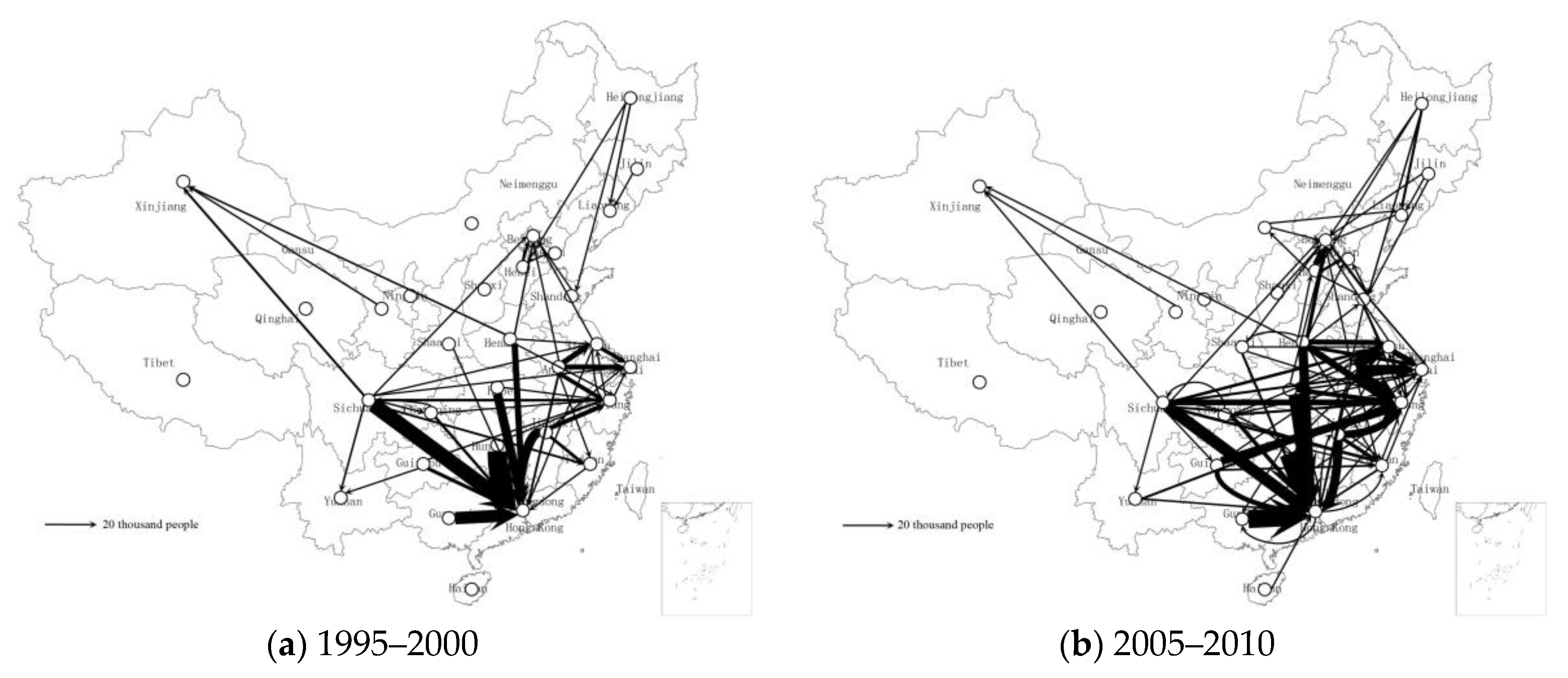
Figure 1 shows the main flows of inter-provincial population migration within China except Hong Kong, Macau and Taiwan. The provinces include Heilongjiang, Jilin, Liaoning, Beijing, Tianjin, Hebei, Shandong, Shanghai, Zhejiang, Jiangsu, Henan, Shanxi, Anhui, Hunan, Hubei, Jiangxi, Guangdong, Fujian, Hainan, Inner Mongolia, Shaanxi, Gansu, Ningxia, Qinghai, Xinjiang, Tibet, Sichuan, Chongqing, Yunnan, Guizhou and Guangxi. The following can be seen in Figure 1.

First of all, people mainly immigrated to three economic circles of Pearl River Delta, Yangtze River Delta and Beijing-Tianjin Area. During 1995 and 2000, the sampled population migrating to these three areas was 1.1501 million, 0.6791 million and 0.2382 million, accounting for 35.63%, 21.04% and 7.38% of the total sampled migrant population in that period of time, respectively. Thus, nearly two thirds of migrants in the country moved to Pearl River Delta, Yangtze River Delta and Beijing-Tianjin Area. Among them, Pearl River Delta was the first choice, followed by Yangtze River Delta. During 2005 and 2010, the figures were 1.3874 million, 1.8161 million and 0.5325 million, accounting for 25.23%, 33.02% and 9.68% of the total sampled migrant population in that period of time, respectively. Three economic circles were still the main destinations but the relative status changed with Yangtze River Delta as the first choice (one third). At the same time, the proportion of the migrant population to three economic circles in the total also increased, indicating the concentration of the inter-provincial population migration.

Secondly, population migration has a certain geographical proximity. It can be seen from Figure 1 that the sampled population immigrating to Pearl River Delta generally came from Hunan, Guangxi, Jiangxi, Sichuan, Hubei and Henan in both periods of time, of whom those coming from Hunan, Guangxi, Jiangxi and Sichuan accounted for 63.39% and 57.49% of the total sampled immigrant population of Guangdong during 1995 and 2000 and during 2005 and 2010, respectively. The sampled population immigrating to the Yangtze River Delta Region generally came from Anhui, Henan, Sichuan, Jiangxi and Guizhou, of whom those coming from Anhui and Henan accounted for 40.10% and 35.05% during 1995–2000 and during 2005–2010, respectively. The sampled population immigrating to the Jing-Jin Area generally came from Hubei, Henan, Shandong and the northeast China, of whom those coming from Hebei, Henan and Shandong accounted for 40.9% and 45.34% of the population during 1995–2000 and during 2005–2010, respectively.

All in all, according to the spatial pattern of China’s inter-provincial population migration, the immigrant areas were mainly concentrated in Pearl River Delta, Yangtze River Delta and the Jing-Jin Area, which were also the main engine of China’s economic development. In 2010, the economic aggregate of these three economic circles accounted for 35.62% of the total in the country and the per capita GDP was 1.77 times more than the national average, ranking top among provinces in the country. Sichuan, Anhui, Hunan, Jiangxi, Guangxi, Chongqing and Guizhou had a high immigration rate (the proportion of the immigrant population of the total population) and their level of economic development was also low with the per capita GDP being only 71.48% of the national level in 2010, in which Guizhou had the lowest per capita GDP. Thus, China’s provincial population migration is closely related with the GDP. People always emigrate from the less developed areas to the well-developed areas with certain geographical proximity.

3.2. Population Migration and Economic Development Level

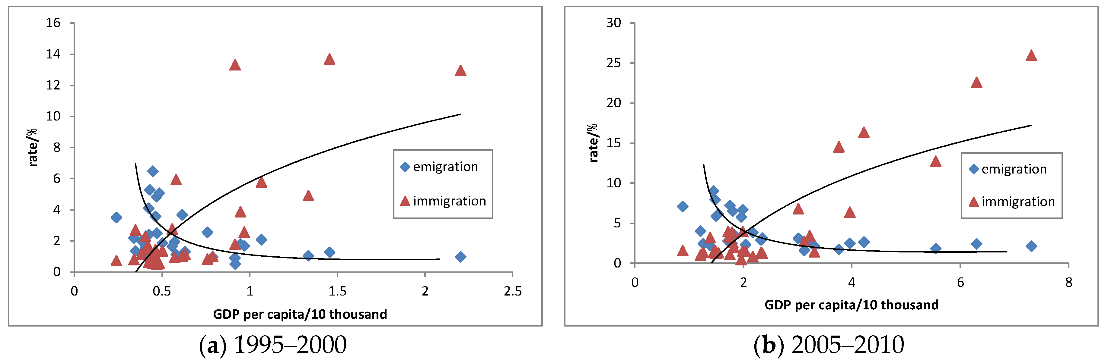
Next, the relationship between the provincial population migration and the per capita GDP of different provinces will be analyzed. With the per capita GDP as the horizontal axis (selecting the middle year of each period of time, namely, 1998 and 2008) and the migration rate (the proportion of emigrants (blue diamond)/immigrants (red triangle) in the total population multiplied by 10, since the data were sampling at 10%) as the longitudinal axis, the scatter plot of the relationship between the provincial population migration and the economic development level during 1995 and 2000 and during 2005 and 2010 can be drawn (Figure 2). It can be found from the figure that:

First of all, the provinces with a high emigration rate were generally less developed and those with the low emigration rate were generally well developed in the same period. For example, during 1995 and 2000, the sampled emigration rate was over 4% in Jiangxi, Sichuan, Hunan, Anhui and Guangxi and the per capita GDP was lower than three quarters of the national level in these provinces; during 2005 and 2010, the figure was over 7% in Anhui, Jiangxi, Hunan and Guizhou and the per capita GDP was lower than three quarters of the national level, too. However, it was lower than 2% in the economically developed areas during 1995 and 2000 and lower than 2.6% during 2005 and 2010, such as Shanghai, Beijing, Tianjin, Zhejiang, Jiangsu and Guangdong. On the other hand, some less developed provinces, such as Ningxia, Yunnan, Gansu and Tibet, also had a low sampled emigration rate. Maybe it was due to their special national cultural characteristics or due to their far distance from the three economic circles. Therefore, except for individual provinces, the inter-provincial population emigration is inversely proportional to the economic development level.

Secondly, the immigration rate is directly proportional to the economic development level in the same period. During 1995 and 2000, the sampled immigration rate was above 12% in economically developed provinces like Beijing, Shanghai and Guangdong; during 2005 and 2010, the figure was above 12% too in Shanghai, Beijing, Zhejiang, Guangdong and Tianjin. But, it was below 0.8% and 1.6% in the less developed areas during 1995 and 2000 and during 2005 and 2010, such as Guizhou, Gansu, Guangxi, Sichuan, Anhui and Jiangxi. However, some provinces had a high sampled immigration rate but their economic development level was not high, such as Xinjiang and Tibet, whose sampled immigration rates were 5.9% and 2.7% during 1995 and 2000, respectively, which was due to China’s political migration; and some provinces had a high level of economic development but the immigration rate was relatively low, such as in Shandong and Jilin, whose per capita GDPs were above the national average.

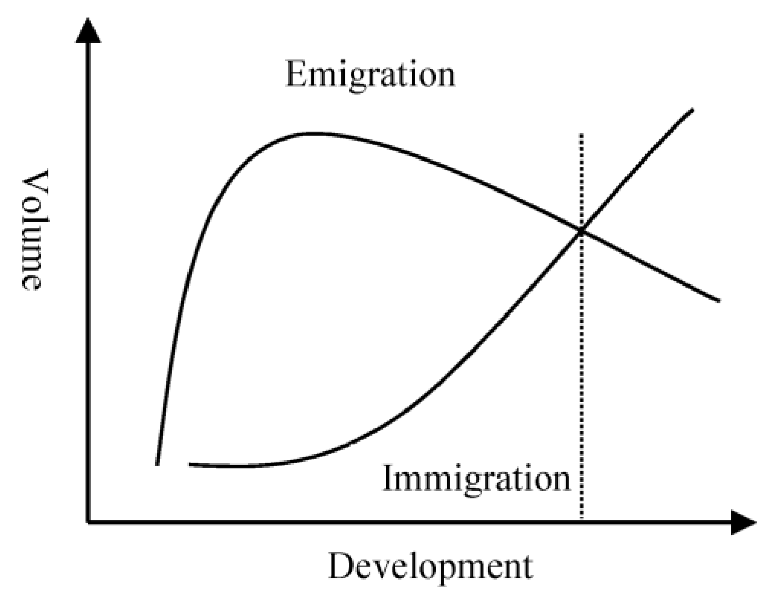
Thirdly, from the historical view, along with the economic development, the population migration level also increases accordingly in the same area. From the period of 1995–2000 to the period of 2005–2010, except in Xinjiang, whose sampled immigration rate decreased obviously, other provinces all had increasing sampled immigration rates and emigration rates to some extent. Nationally, during 1995 and 2000, the national sampled migration population accounted for 2.56% of the total; the proportion increased to 4.20% during 2005 and 2010. Thus, China’s inter-provincial population migration level increases with the economic development level, which is consistent with the initial stage of the general law of international population migration. According to the research of Hein, with the economic development of a country or a region, the immigrant population showed an inverted U curve, which increased initially and decreased afterwards; and the population immigration basically increased with economic development (Figure 3). The whole process could be divided into three stages: the initial stage, when migration costs decreased due to economic development, the emigration population increased rapidly and the immigration population increased slowly; the mid-stage, when the economy developed to a certain extent, the emigration population began to decrease and the immigration population began to increase rapidly but the former was still greater than the latter; the late stage, when the economy was highly developed, the emigration population continued to decrease and the immigration population continued to increase; and, the latter was greater than the former. It can be seen from the foregoing analysis that China’s inter-provincial population migration was basically in the initial stage.

In brief, China’s inter-provincial population migration has the following laws: laterally, the higher the level of economic development is, the lower the emigration rate and the higher the immigration rate is; historically, with economic development, both emigration and immigration levels increase. The conclusion seems to be contradictory but it is easy to understand, because all provinces have the consistent population migration curve (Figure 3) with the change of economic development historically, but they have different economic levels at the same time and sequenced differences in the inter-provincial migration levels.

4. The Spatio-Temporal Model for Migration

The above analysis shows that China’s inter-provincial population migration is related to not only the distance between provinces but also the regional economic development level. Thus, the modeling analysis below will consider distance and per capita GDP.

4.1. Model A: The General Regression Model

The variable of per capital GDP is introduced according to the traditional inter-regional migration gravity model formula to build the following model:

$$m_{ij}={\beta }_0{g}_i^{{\beta }_1}{g}_j^{{\beta }_2}{p}_i^{{\beta }_3}{p}_j^{{\beta }_4}{d}_{ij}^{{\beta }_5}$$

(1)

where m_ij represents the total population emigrating from i to j; g_i and g_j represent the per capita GDPs of i and j, respectively; p_i and p_j represent the total population of i and j, respectively; d_ij represents the distance between i and j; β₀, β₁, β₂, β₃, β₄ and β₅ are all coefficients.

Take the logarithm for Formula (1) to get:

$$\ln (m_{ij})={\beta }_0+{\beta }_1\ln (g_i)+{\beta }_2\ln (g_j)+{\beta }_3\ln (p_i)+{\beta }_4\ln (p_j)+{\beta }_5\ln (d_{ij})+\epsilon$$

(2)

Suppose there are n areas, so N groups of formulas can be written according to Formula (2) (N = n × n, the population migration from self to self is assumed to be 0 first, to facilitate the introduction of space weight matrix later—the same in the below model—then the self-migration is removed from the sample data), as shown in

Table 1. Structure of sample data for migration.

Dyad Label	ID Origin	ID Destination	Flows	Origin Variables		Destination Variables		Distance Variable
				Population	GDP per Capita	Population	GDP per Capita
1	1	1	m11	p1	g1	p1	g1	d11
$⋮$	$⋮$	$⋮$	$⋮$	$⋮$	$⋮$	$⋮$	$⋮$	$⋮$
n	1	n	m1n	p1	g1	pn	gn	d1n
N + 1	2	1	m21	p2	g2	p1	g1	d21
$⋮$	$⋮$	$⋮$	$⋮$	$⋮$	$⋮$	$⋮$	$⋮$	$⋮$
2n	2	n	m2n	p2	g2	pn	gn	d2n
$⋮$	$⋮$	$⋮$	$⋮$	$⋮$	$⋮$	$⋮$	$⋮$	$⋮$
N – n + 1	n	1	mn1	pn	gn	p1	g1	dn1
$⋮$	$⋮$	$⋮$	$⋮$	$⋮$	$⋮$	$⋮$	$⋮$	$⋮$
N	n	n	mnn	pn	gn	pn	gn	dnn

Source: the authors made it by themselves.

. It can be expressed as below with the matrix:

$$M={\beta }_0{L}_n+{\beta }_1{X}_1+{\beta }_2{X}_2+{\beta }_3{X}_3+{\beta }_4{X}_4+{\beta }_5{X}_5+\epsilon$$

(3)

where M is a N × 1 matrix, representing the total migration population between two regions; L_n represents the N × 1 matrix whose element is 1; both X₁ and X₂ are the N × 1 matrix, representing the per capita GDPs of the emigration place and the immigration place, respectively; X₃ and X₄ represent the population sizes of the emigration place and the immigration place, respectively, being a N × 1 matrix; X₅ represents the distance between two regions, being a N × 1 matrix.

4.2. Model B: The Extension Regression Model Considering the Historical Factor

As stated earlier, many scholars believe that the introduction of the historical variable in the gravity model can not only improve the model’s accuracy but also explains well the migration law (Fan, 2005 [34]). Since there are data of the inter-provincial population migration over two periods, the first one can be taken as the historical variable and the population migration of the second period is modeled. Based on Formula (3), the formula during 2005 and 2010 can be expressed as:

$$M={\beta }_0{L}_n+{\beta }_1{X}_1+{\beta }_2{X}_2+{\beta }_3{X}_3+{\beta }_4{X}_4+{\beta }_5{X}_5+{\beta }_6{M}_{t-1}+\epsilon$$

(4)

where M_t−1 is the inter-provincial population migration during 1995 and 2000, being a N × 1 matrix; β₆ is a coefficient. Formula (4) is the extension regression model considering the historical variable.

4.3. Model C: The Spatial Lag Regression Model

In general, in the case of knowing enough samples, Formula (3) can be solved by the least squares method but the premise is that there is no correlation between the samples. In the actual situation, the inter-regional population migration has much to do with the geographical proximity, showing the obvious space correlation. In order to take the space correlation into account, the spatial lag model is introduced here to make the spatial lag regression estimate on the parameter.

The spatial lag model is to reflect the influence of the geographical position on regression parameters by introducing the spatial autocorrelation factor W to the regression model, namely, Y = p × W × Y + b × X + ε, in which W means the spatial weight matrix. The essence is to give the geographical weight to a sample point and proximal points within a certain space range and then make the least-squares regression, namely, making a regression on each sample point with different regression parameters. However, the inter-regional population migration involves the flow between two points rather than on an observation point, so it is more complicated. LeSage and Pace [55,56] once estimated the O-D flow by introducing three spatial lag factors to represent the outflow point, the inflow point and the influence of spatial correlation on. With the help of their thoughts, some scholars have studied China’s inter-provincial trade flow issue [53]. Here, the above method is used to assume the space weighted matrix to be W and introduce three spatial lag factors on the basis of Formula (3):

$$M={\beta }_0{L}_n+{\rho }_0{W}_{0}M+{\rho }_d{W}_{d}M+{\rho }_w{W}_{w}M+{\beta }_1{X}_1+{\beta }_2{X}_2+{\beta }_3{X}_3+{\beta }_4{X}_4+{\beta }_5{X}_5+\epsilon$$

(5)

where $W_0=W\otimes I_n$, W is the n × n matrix, representing the space weight and the diagonal element is zero; I_n is the unit matrix; $\otimes$ is the Kronecker product of the matrix, namely, the matrix obtained by multiplying each element of the weight matrix W by I_n, so W₀ is a N × N matrix; since M is the N × 1 matrix, $W_{0}M$ is a N × 1 matrix and its element is the weighting sum of M with the space weight between the emigration space and other places as the weight, so it represents the spatial dependence of population migration on the emigration space; similarly, $W_d=I_n\otimes W$, $W_{d}M$ is a N × 1 matrix and its element is the weighting sum of M with the space weight between the emigration space and other places as the weight, so it represents the spatial dependence of population migration on the immigration space; $W_w=W\otimes W$; $W_{w}M$ is also a N × 1 matrix and its element is the weighting sum of M with the space weight between the emigration space and the immigration space, so it represents the spatial dependence of population migration on the migration flow itself. Finally, the migration data between self and self are removed from all N × 1 matrixes above to avoid the error.

The spatial weight matrix W describes the change of the importance of the sample points to the estimated points with the increase of distance between them. The core of the spatial lag regression model is the selection of the spatial weight matrix, which is to express the different understandings of the spatial relationship between data by selecting different spatial weight functions [57]. The spatial lag regression results have great dependence on the selection of the spatial weight function. In the spatial lag regression analysis, there are many spatial weight function forms with the Gauss weight function as one of the most commonly used methods. The basic idea of the Gauss weight function is to express the relationship between the spatial weight w_ij and the distance d_ij by selecting a continuous, monotone decreasing function. The form of the function is as follows [58]:

$$w_{ij}=\exp (-(1/2){(d_{ij}/b)}^2)$$

(6)

where b is a non-negative attenuation parameter describing the functional relationship between weight and distance, known as Bandwidth, as shown in Figure 4. For a given bandwidth, when d_ij = 0, w_ij = 1 and the weight is the largest; with the increasing distance between the data point and the regression point, w_ij decreases gradually; when point j is far away from point i, w_ij is close to zero. In other words, these points have near little impact on the parameters of the regression points. The greater the bandwidth is, the slower the weight decreases with the increasing distance; the smaller the bandwidth is, the faster the weight decreases with the increasing distance. When the bandwidth is 0, only the weight of the regression point i is 1 and the weight of the others approaches 0; the data regression process is just the re-expression of the observation value; when the bandwidth approaches infinity and the weights of all observation points approach 1, which generates a general regression model. Therefore, the selection of bandwidth has great influence on the spatial lag regression results. The bandwidth in this paper is selected according to the population migration sample data. As stated above, China’s inter-provincial population migration has certain geographical proximity. According to the general distance of the inter-provincial population migration, the bandwidth b is 1000 km. After the bandwidth is determined, the spatial weight matrix W can be obtained. Finally, the diagonal element is set to be zero. In order to make the weight of all sample points around the estimate point add up to be 1, it needs to make the normalization processing on W.

5. Case Study for China’s Inter-Provincial Migration

5.1. Data Source and Specification

The inter-provincial population migration data are from the sampled population migration statistics, based on the place of current residence and the place of residence five years ago in the 5th and 6th population census of China, that is, the inter-provincial population migration sampled data during 1995 and 2000 and during 2005 and 2010. The Chinese national statistics department conducts a large-scale population census every decade (sample population is 10% of the total population). Each census is attended by all government statistical department staff and many social volunteers to ensure the accuracy of the data. So far, six national censuses have taken place. Migration is one of the main statistical indicators of census work. Therefore, the quality of the population migration data used in this paper is relatively high.

With reference to the processing methods of other scholars [34], the total population and per capita GDP of the provincial administrative regions are from the China Statistical Yearbook in the middle year of each period of time. In other words, the data in 1998 and in 2008 are taken during 1995 and 2000 and during 2005 and 2010, respectively; the distance between regions uses the average value of the railway and highway mileage between the capital cities of different provinces in the corresponding year; the railway and highway mileage is from the railway and roadway mileage table between major cities of China in the Chinese traffic map in the corresponding year. In addition, considering it takes about 10 hours to Qiongzhou Strait by ferry, the distance is taken as 1000 km.

5.2. Results Analysis

It can be found, according to the regression result of the mode, (

Table 2. Comparison of outcomes of different models.

	Model A				Model B		Model C
	1995–2000		2005–2010		2005–2010		1995–2000		2005–2010
	B a	t b	B a	t b	B a	t b	B a	t b	B a	t b
constant	−2.68	−2.02 *	−2.614	−2.10 *	−0.825	−1.29	12.550	11.11 ***	13.57	11.38 ***
W0M							0.885	22.34 ***	0.889	22.93 ***
WdM							0.922	19.51 ***	0.704	13.34 ***
WwM							−1.186	−15.10 ***	−1.032	−13.35 ***
wi	−0.453	−6.30 ***	−0.446	−7.59 ***	−0.079	−2.53 ***	−0.252	−4.86 ***	−0.328	−7.26 ***
wj	1.100	15.29 ***	1.121	19.06 ***	0.409	12.22 ***	0.047	0.643	0.075	1.11
pi	0.856	19.39 ***	0.830	21.49 ***	0.215	9.18 ***	0.022	0.418	0.176	3.22 **
pj	0.567	12.86 ***	0.436	11.28 ***	−0.012	−0.55	0.029	0.734	0.004	0.103
dij	−0.969	−18.54 ***	−0.879	−19.55 ***	−0.191	−7.06 ***	−0.945	−22.69 ***	−0.937	−25.79 ***
Mt−1					0.717	49.16 ***
R2	0.643		0.690		0.918		0.825		0.830
Ad R2	0.641		0.688		0.918		0.824		0.829
F-test	311.8 ***		385.1 ***		1620.9 ***		508.2 ***		526.1 ***

Note: ^a Regression coefficient; ^b t-test, *** Significance level < 0.001, ** Significance level < 0.01, * Significance level < 0.1.

) that, first of all, the regression effects of the extension regression model and the spatial lag regression model increase greatly from 0.6–0.7 to 0.8–1.0 by adjusted R² compared with the general models. It also proves that population migration has strong spatial properties. In the modeling and prediction of population migration, introducing the spatial factors can improve the modeling and prediction accuracy.

Secondly, the regression results verify the relationship between China’s inter-provincial population migration and the regional economic development level: population migration is negatively correlated with the economic development level of the emigration place and positively correlated with that of the immigration place. At the same time, it also proves that the inter-provincial population migration is positively correlated with the population size of the immigration and emigration places and negatively correlated with the distance between the emigration place and the immigration place. The regression results of three models all show that the coefficients of both W_i and d_ij are negative and the significance level is below 0.001. The regression coefficients of three factors, namely, w_j, p_i and p_j, are positive and significant only in Model A; some factors cannot pass the t-test in Model B and C, because the introduction of the spatial factors (the historical variable is also a spatial factor without weight) will cause an interaction between factors due to the spatial self-correlation of other factors, thus affecting the regression result.

Thirdly, the historical factors and the spatial lag factors can explain the migration between regions to a great extent. In Model B, the regression coefficient of the factor M_t−1 is positive, indicating that the history of the population migration has a positive influence on the later migration. It also shows the path dependence of China’s inter-provincial population migration, which means migration used to move to the destination of previous migrations, which populations were familiar with from their social networks. In Model C, the spatial lag factors of W₀M, W_dM and W_wM also have a strong significance level, indicating the high explanatory degree of the spatial lag factor on population migration. The positive regression coefficients of W₀M and W_dM show that a large population immigration or emigration size in two adjacent areas of a region will lead to the mass population emigration or immigration here. In other words, population migration has the spatial self-correlation. Of course, it is also related to the self-correlation of the economic development level.

Generally, the adjacent provinces in China have a similar economic development level. For example, the provinces in the East are economically developed and those in central and southwest China are less developed. Due to the great correlation between population migration and economic development level, the spatial self-correlation of economic development level affects that of population migration to a certain extent. That’s why the significant level of other variables is not high after introducing the spatial factors.

6. Discussion

China’s sampled inter-provincial population migration data during 1995 and 2000 and during 2005 and 2010 are analyzed in this paper. The results show that: first of all, the inter-provincial population increases rapidly in size with strong geographical proximity; secondly, population migration is closely related to the economic development level. Vertically, with economic development, the inter-provincial population emigration and immigration levels increase greatly; in the same period, the economically developed areas have a low emigration level and a high immigration level, and the less developed areas have a high emigration level and a low immigration level. These features reflect that China’s inter-provincial population migration is still in the initial stage of the general process of population migration.

The regression model is conducted on China’s inter-provincial population migration data in two periods by establishing the general regression model, the extension regression model, considering the historical dependent variable, and the spatial lag regression model, considering the spatial lag factor. The results not only prove the relationship between China’s inter-provincial population migration and the regional economic development level but also find that the introduction of the historical dependent variable or the spatial lag factor can greatly improve the modeling accuracy of the model and the spatial factor have stronger explanatory ability than the historical variable on the issue of inter-provincial population migration. Introduction of spatial factors to the inter-regional migration model is one of the main contributions of this paper, and the results of this paper not only have some academic significance but also provide some strong revelations for migration policy-making in practice.

In academic terms, the above results tell us that we must consider both time and space factors when establishing the population prediction model, because these two factors have a great impact on the accuracy of the model. In practice, they provide some enlightenment for regional population migration policy-making and regional development planning. First, the historical features of inter-regional migration should be taken into full consideration in the formulation of the migration policy, as migration generally has a path-dependent character. If the migration policy can adapt to this path dependence, then the effect will be very good. But if it is inconsistent with this path dependence, it will have a poor policy effect. Second, in regional development planning, population migration should be promoted from the perspective of shortening the spatial distance because space factors are crucial factors in population migration. For example, the construction of the high-speed railway in China has a great impact on shortening the spatial distance, which is bound to affect inter-regional population migration.

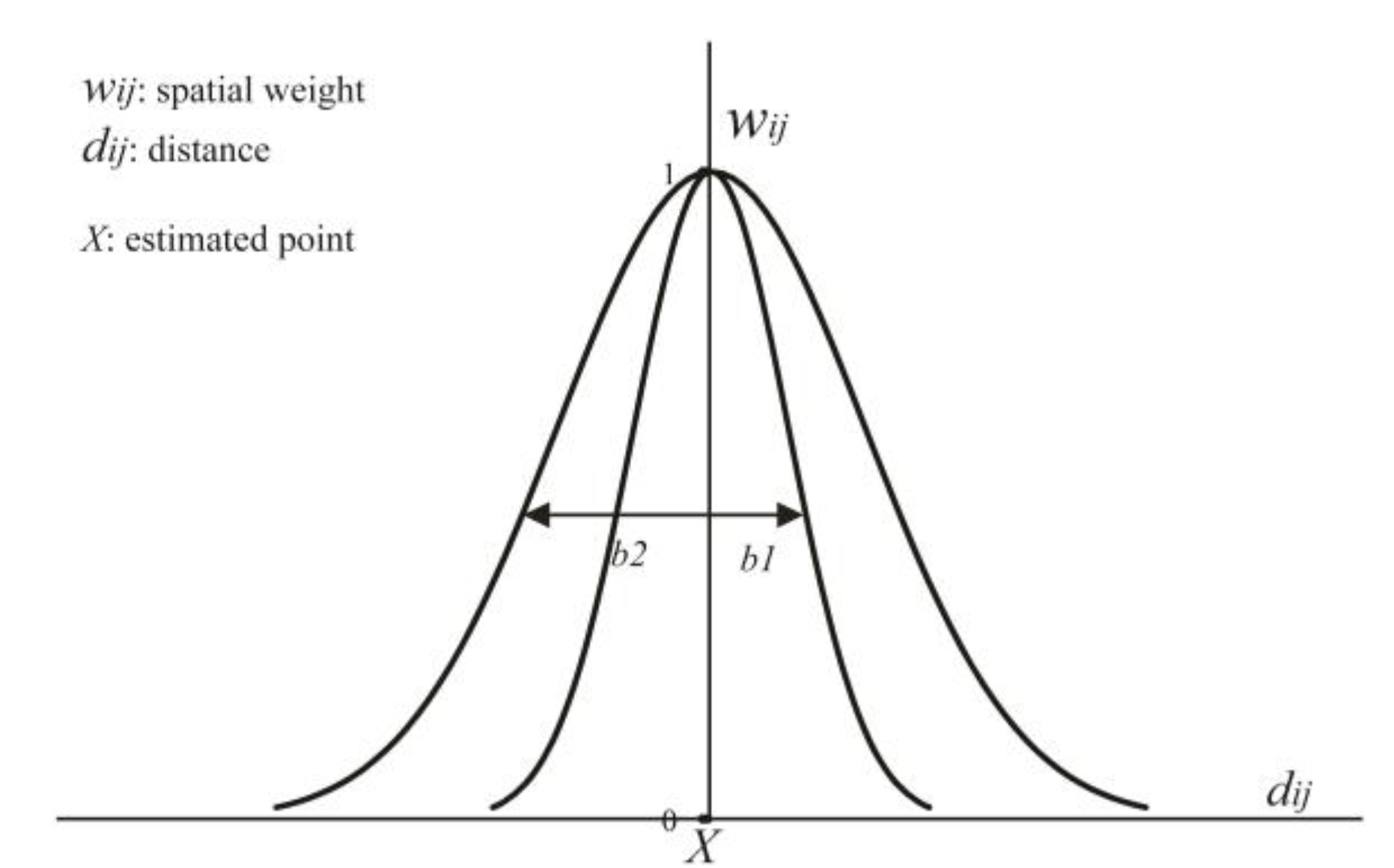
Using the geographical weight can improve the modeling effect of the model but it needs further study and improvement. The first improvement is to understand how to select the optimal bandwidth b in the spatial weight matrix. Bandwidth selection has a great impact on the regression result of the geographical weight. There are some principles for the bandwidth selection of weight functions in math, such as AIC and BIC, which needs further study and discussion because the bandwidth in our spatial lag model is determined empirically. The second is how to deal with the spatial self-correlation of factors and the correlation of factors in the spatial lag regression. Factors like population and economy usually have a certain spatial self-correlation; at the same time, there is certain correlation between factors; how to deal with the relationship between factors after introducing the spatial factor still needs further research.