Changes in the Ecological Environment of the Marginal Seas along the Eurasian Continent from 2003 to 2014

Abstract
:1. Introduction
2. Materials and Methods
2.1. Satellite Data Acquisition
2.2. Satellite Retrieval of the SDD
2.3. Statistical Analyses
3. Results
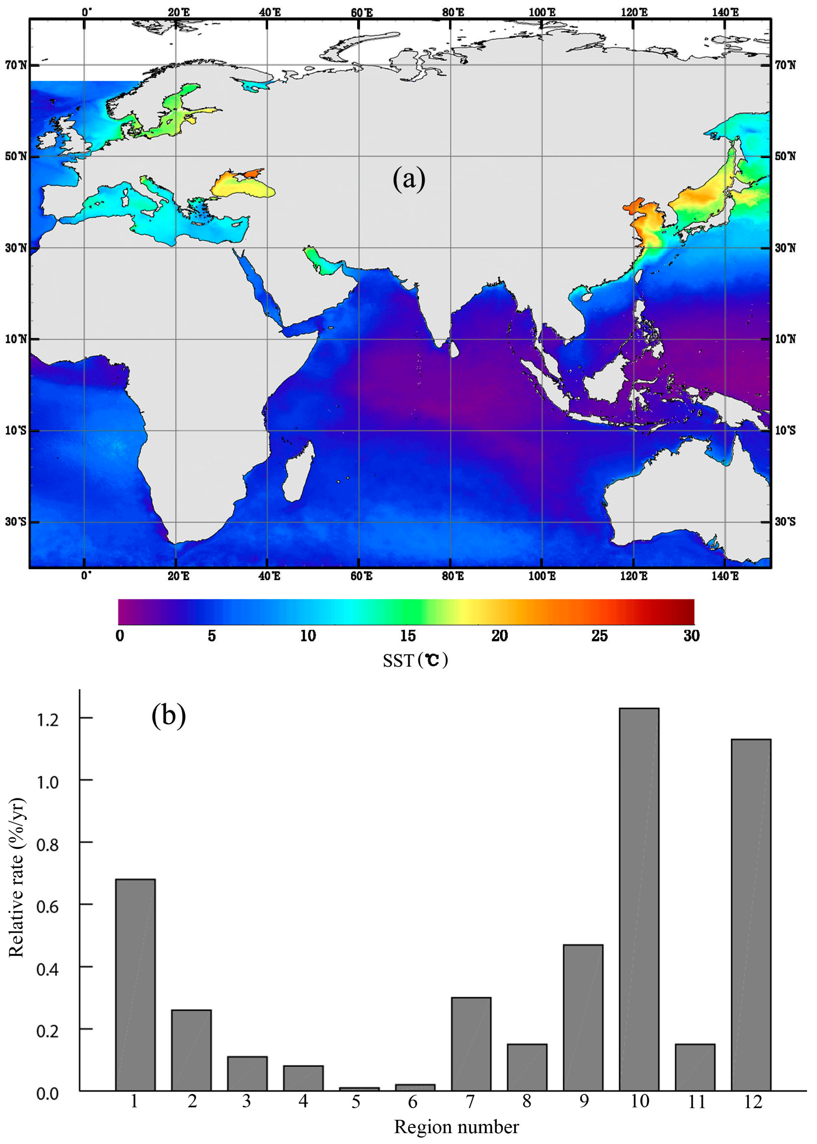
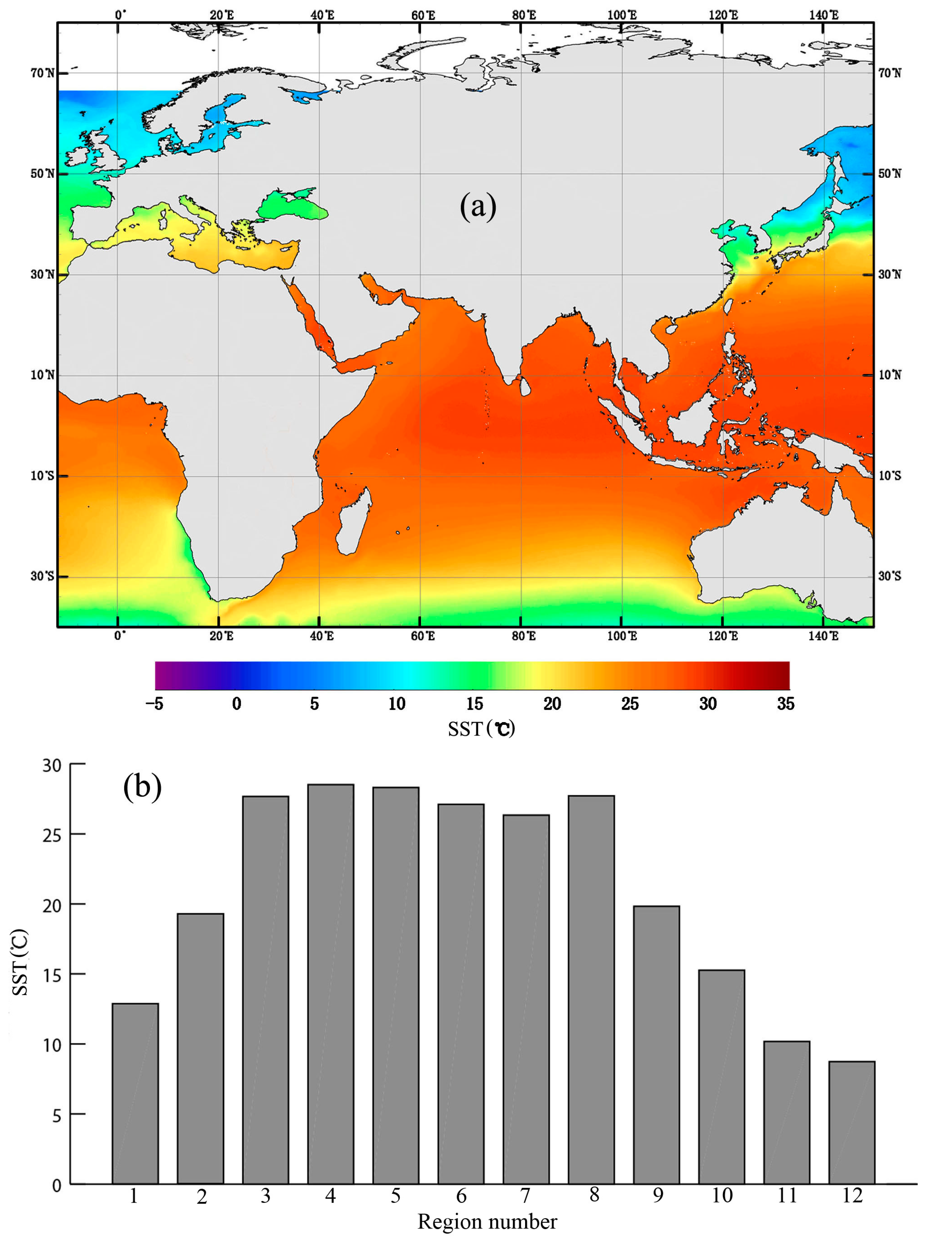
3.1. Changes in SST
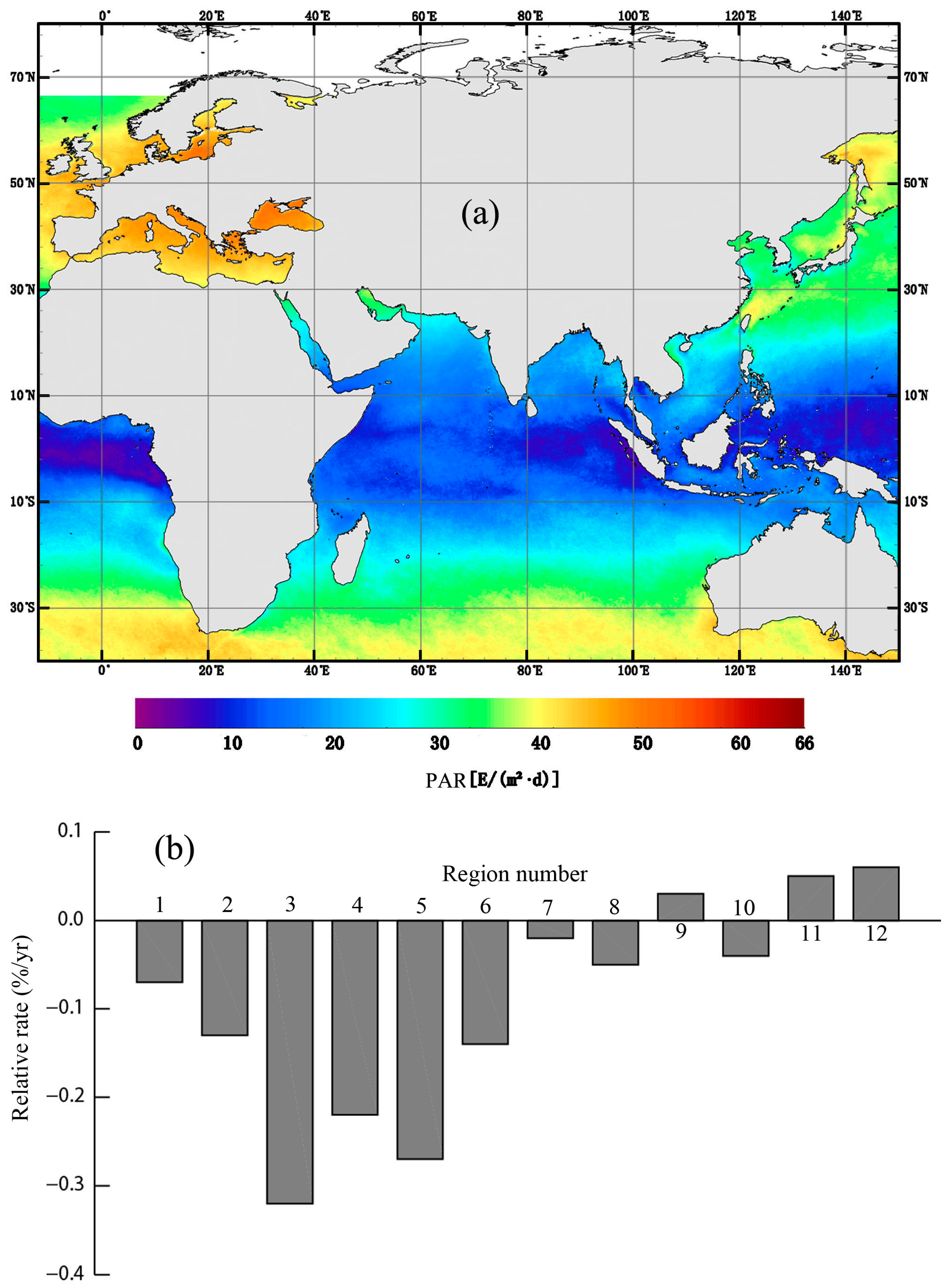
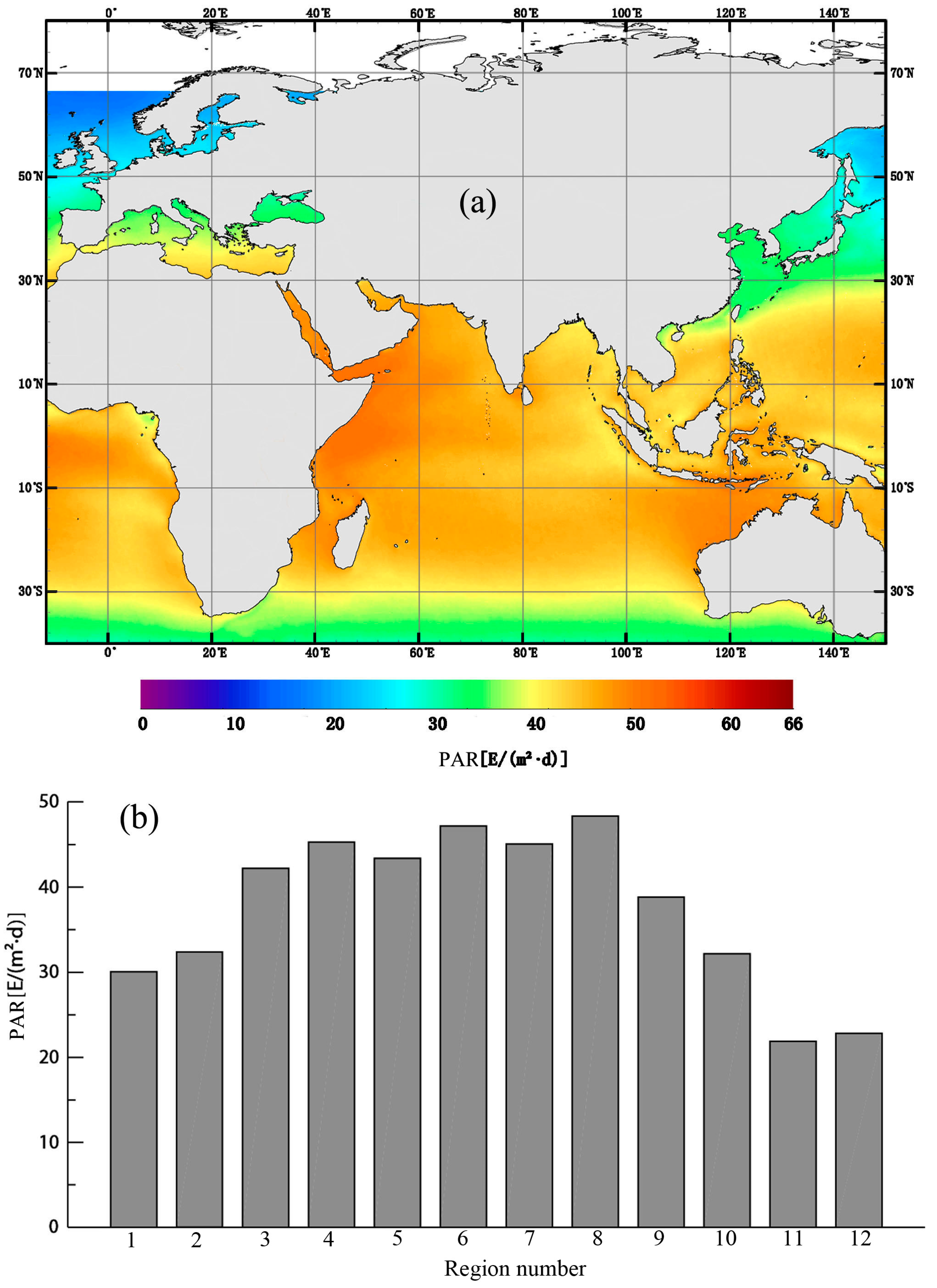
3.2. Changes in PAR
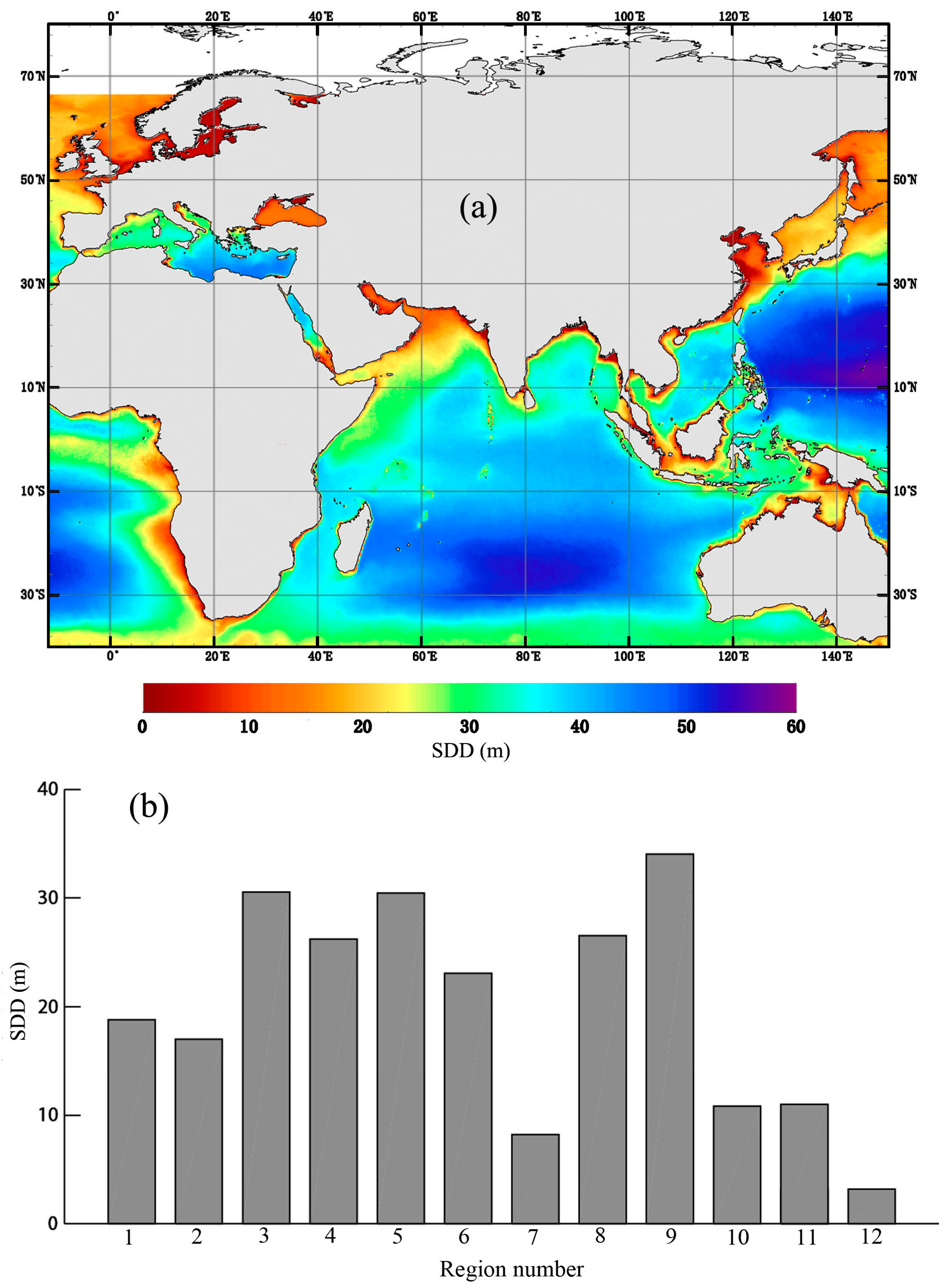
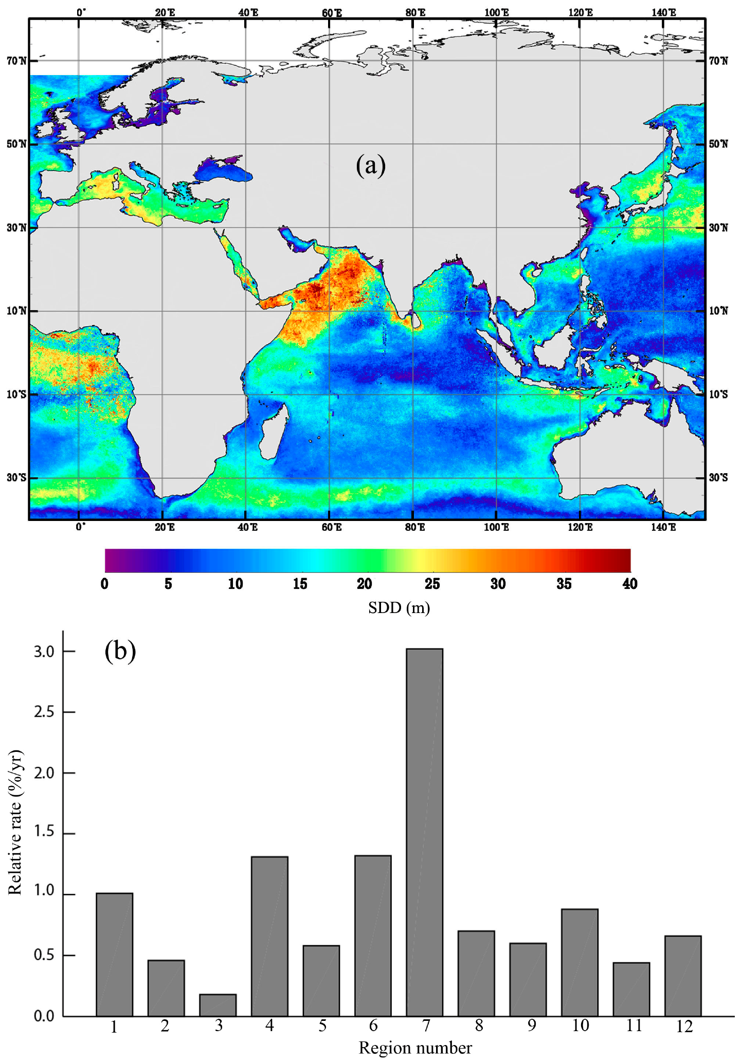
3.3. Changes in SDD
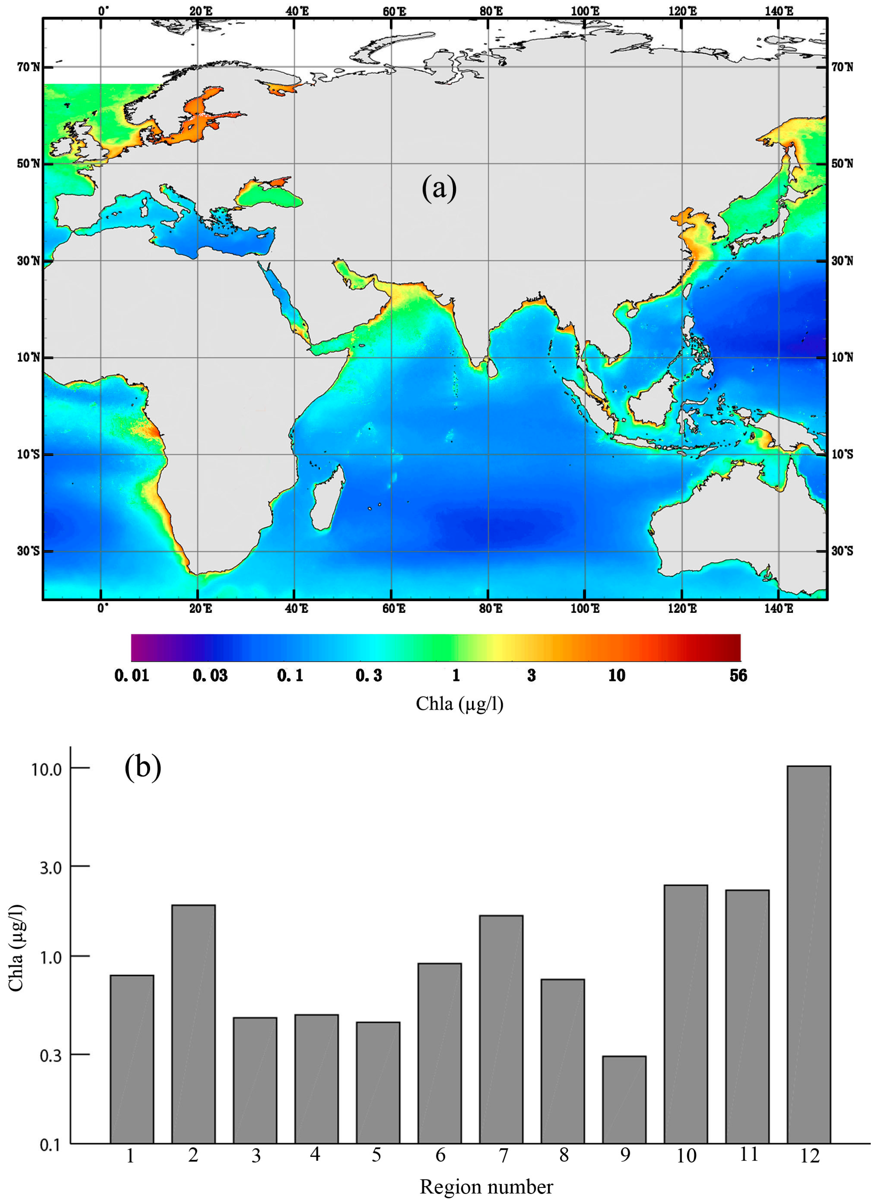
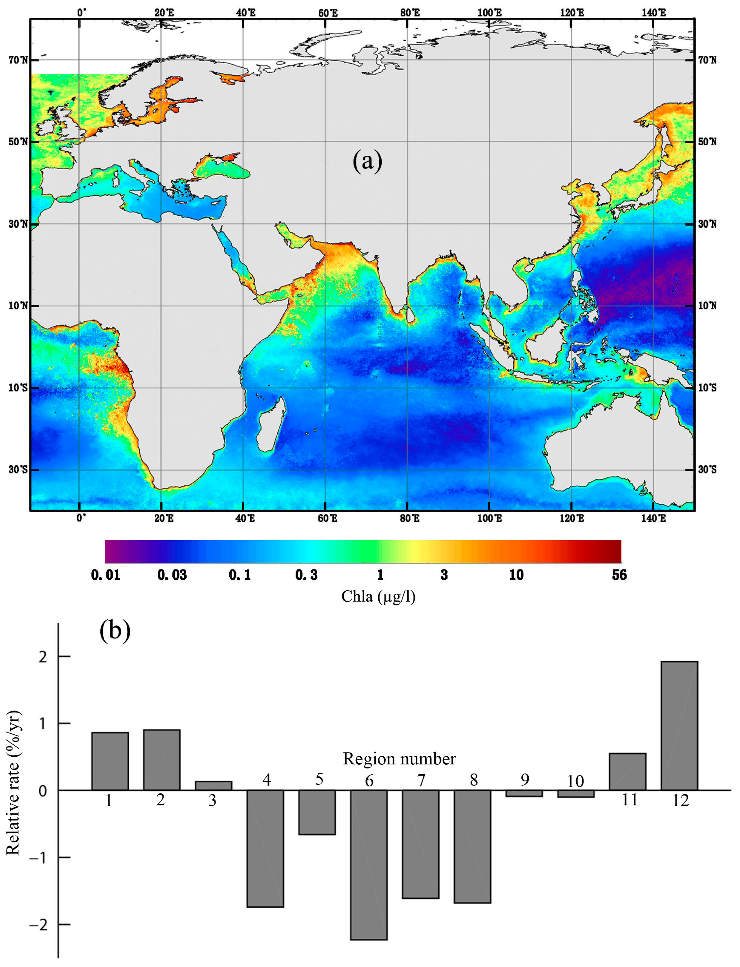
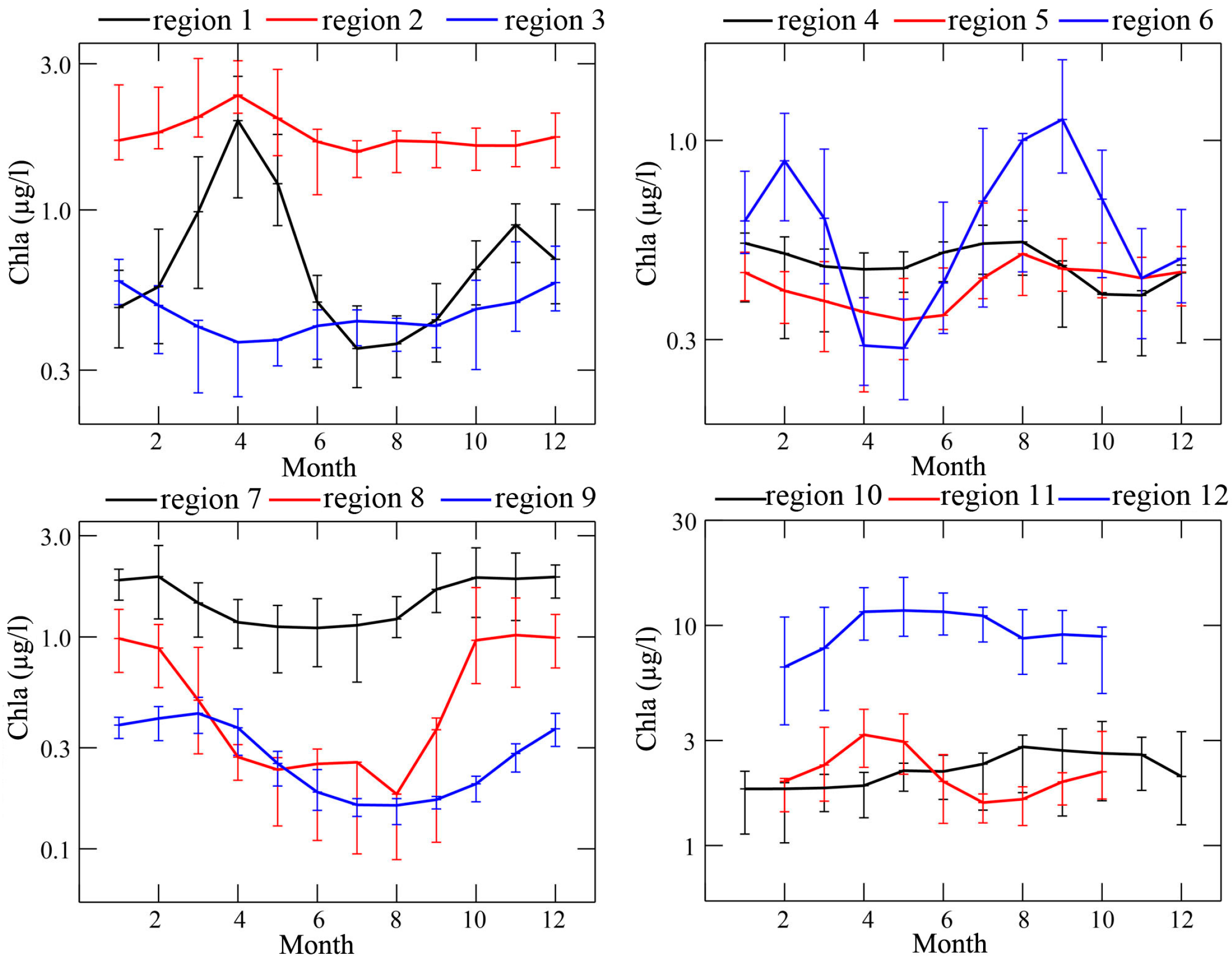
3.4. Changes in Chla
4. Discussion
5. Conclusions
Acknowledgments
Author Contributions
Conflicts of Interest
References
- Spalding, M.D.; Ravilious, C.; Green, E.P. United Nations Environment Programme, World Conservation Monitoring Centre. World Atlas of Coral Reefs; University of California Press: Berkeley, CA, USA, 2001. [Google Scholar]
- Burke, L.; Reytar, K.; Spalding, M.; Perry, A. Reefs at Risk Revisited; World Resources Institute: Washington, DC, USA, 2011; p. 114. [Google Scholar]
- Veron, J.; Stafford-Smith, M.; DeVantier, L.; Turak, E.E. Overview of distribution patterns of zooxanthellate Scleractinia. Front. Mar. Sci. 2015, 1, 81. [Google Scholar] [CrossRef]
- Giri, C.; Ochieng, E.; Tieszen, L.L.; Zhu, Z.; Singh, A.; Loveland, T.; Masek, J.; Duke, N. Status and distribution of mangrove forests of the world using earth observation satellite data. Glob. Ecol. Biogeogr. 2011, 20, 154–159. [Google Scholar] [CrossRef]
- Short, F.; Carruthers, T.; Dennison, W.; Waycott, M. Global seagrass distribution and diversity: A bioregional model. J. Exp. Mar. Biol. Ecol. 2007, 350, 3–20. [Google Scholar] [CrossRef]
- Behrenfeld, M.J.; O’Malley, R.T.; Siegel, D.A.; McClain, C.R.; Sarmiento, J.L.; Feldman, G.C.; Milligan, A.J.; Falkowski, P.G.; Letelier, R.M.; Boss, E.S. Climate-driven trends in contemporary ocean productivity. Nature 2006, 444, 752–755. [Google Scholar] [CrossRef] [PubMed]
- McClain, C.R.; Signorini, S.R.; Christian, J.R. Subtropical gyre variability observed by ocean-color satellites. Deep Sea Res. Part II 2004, 51, 281–301. [Google Scholar] [CrossRef]
- Polovina, J.J.; Howell, E.A.; Abecassis, M. Ocean’s least productive waters are expanding. Geophys. Res. Lett. 2008, 35, L03618. [Google Scholar] [CrossRef]
- Irwin, A.J.; Oliver, M.J. Are ocean deserts getting larger? Geophys. Res. Lett. 2009, 36, L18609. [Google Scholar] [CrossRef]
- Steinacher, T.K.; Joos, M.F.; Frolicher, T.L.; Bopp, L.; Cadule, P.; Cocco, V.; Doney, S.C.; Gehlen, M.; Lindsay, K.; Moore, J.K.; et al. Projected 21st century decrease in marine productivity: A multi-model analysis. Biogeosciences 2010, 7, 979–1005. [Google Scholar] [CrossRef] [Green Version]
- Boyce, D.G.; Lewis, M.R.; Worm, B. Global phytoplankton decline over the past century. Nature 2010, 466, 591–596. [Google Scholar] [CrossRef] [PubMed]
- Gregg, W.W.; Conkright, M.E. Decadal changes in global ocean chlorophyll. Geophys. Res. Lett. 2002, 29. [Google Scholar] [CrossRef]
- Sarmiento, J.L.; Slater, R.; Barber, R.; Doney, S.C.; Hirst, A.C.; Kleypas, J.; Matear, R.; Mikolajewicz, U.; Monfray, P.; Soldatov, V.; et al. Response of ocean ecosystems to climate warming. Glob. Biogeochem. Cycles 2004, 18, GB3003. [Google Scholar] [CrossRef]
- Gregg, W.W.; Casey, N.W.; McClain, C.R. Recent trends in global ocean chlorophyll. Geophys. Res. Lett. 2005, 32, L03606. [Google Scholar] [CrossRef]
- Chavez, F.P.; Messié, M.; Pennington, J.T. Marine primary production in relation to climate variability and change. Annu. Rev. Mar. Sci. 2011, 3, 227–260. [Google Scholar] [CrossRef] [PubMed]
- Siegel, D.A.; Behrenfeld, M.J.; Maritorena, S.; McClain, C.R.; Antoine, D.; Bailey, S.W.; Bontempi, P.S.; Boss, E.S.; Dierssen, H.M.; Doney, S.C.; et al. Regional to global assessments of phytoplankton dynamics from the SeaWiFS mission. Remote Sens. Environ. 2013, 135, 77–91. [Google Scholar] [CrossRef]
- Kahru, M.; Mitchell, B.G. Ocean color reveals increased blooms in various parts of the world. EOS Trans. AGU 2008, 89, 170. [Google Scholar] [CrossRef]
- He, X.; Bai, Y.; Pan, D.; Chen, C.-T.A.; Cheng, Q.; Wang, D.; Gong, F. Satellite views of the seasonal and interannual variability of phytoplankton blooms in the eastern China seas over the past 14 years (1998–2011). Biogeosciences 2013, 10, 4721–4739. [Google Scholar] [CrossRef]
- Yamada, K.; Ishizaka, J. Estimation of interdecadal change of spring bloom timing, in the case of the Japan Sea. Geophys. Res. Lett. 2006, 33, L02608. [Google Scholar] [CrossRef]
- Prakash, P.; Prakash, S.; Rahaman, H.; Ravichandran, M.; Nayak, S. Is the trend in chlorophyll-a in the Arabian Sea decreasing? Geophys. Res. Lett. 2012, 39, L23605. [Google Scholar] [CrossRef]
- Moradi, M.; Kabiri, K. Spatio-temporal variability of SST and Chlorophyll-a from MODIS data in the Persian Gulf. Mar. Pollut. Bull. 2015, 98, 14–25. [Google Scholar] [CrossRef] [PubMed]
- Volpe, G.; Nardelli, B.B.; Cipollini, P.; Santoleri, R.; Robinson, I.S. Seasonal to interannual phytoplankton response to physical processes in the Mediterranean Sea from satellite observations. Remote Sens. Environ. 2012, 117, 223–235. [Google Scholar] [CrossRef]
- Fleming-Lehtinen, V.; Laamanen, M. Long-term changes in Secchi depth and the role of phytoplankton in explaining light attenuation in the Baltic Sea. Estuar. Coast. Shelf Sci. 2012, 102–103, 1–10. [Google Scholar] [CrossRef]
- He, X.; Pan, D.; Mao, Z. Water transparency (Secchi depth) monitoring in the China Sea with the SeaWiFS satellite sensor. Proc. SPIE 2004, 5568, 112–122. [Google Scholar]
- He, X.; Bai, Y.; Chen, C.-T.A.; Hsin, Y.-C.; Wu, C.-R.; Zhai, W.; Liu, Z.; Gong, F. Satellite views of the episodic terrestrial material transport to the southern Okinawa Trough driven by typhoon. J. Geophys. Res. Oceans 2014, 119, 4490–4504. [Google Scholar] [CrossRef]
- He, X.; Pan, D.; Bai, Y.; Wang, T.; Chen, C.-T.A.; Zhu, Q.; Hao, Z.; Gong, F. Recent changes of global ocean transparency observed by SeaWiFS. Cont. Shelf Res. 2017, 143, 159–166. [Google Scholar] [CrossRef]
- Doron, M.; Babin, M.; Hembise, O.; Mangin, A.; Garnesson, P. Ocean transparency from space: Validation of algorithms estimating Secchi depth using MERIS, MODIS and SeaWiFS data. Remote Sens. Environ. 2011, 5, 2986–3001. [Google Scholar] [CrossRef]
- Banse, K.; McClain, C.R. Winter blooms of phytoplankton in the Arabian Sea as observed by the Coastal Zone Color Scanner. Mar. Ecol. Prog. Ser. 1986, 34, 201–211. [Google Scholar] [CrossRef]
- Yang, S.L.; Zhang, J.; Zhu, J.; Smith, J.P. Impact of dams on Yangtze River sediment supply to the sea and delta intertidal wetland response. J. Geophys. Res. Oceans 2005, 110, F03006. [Google Scholar] [CrossRef]
- Bai, Y.; Pan, D.; Cai, W.J.; He, X.; Wang, D.; Tao, B.; Zhu, Q. Remote sensing of salinity from satellite-derived CDOM in the Changjiang River dominated East China Sea. J. Geophys. Res. Oceans 2013, 118, 227–243. [Google Scholar] [CrossRef]
- Bai, Y.; He, X.; Pan, D.; Chen, C.T.A.; Kang, Y.; Chen, X.; Cai, W.J. Summertime Changjiang River plume variation during 1998–2010. J. Geophys. Res. Oceans 2014, 119, 6238–6257. [Google Scholar] [CrossRef]
- Trenhaile, A.S. Coastal Dynamics and Landforms; Clarendon: Oxford, UK, 1997. [Google Scholar]
- Cheung, W.W.L.; Watson, R.; Morato, T.; Pitcher, T.J.; Pauly, D. Intrinsic vulnerability in the global fish catch. Mar. Ecol. Prog. Ser. 2007, 333, 1–12. [Google Scholar] [CrossRef]
- Behrenfeld, M.J.; Falkowski, P.G. Photosynthetic rates derived from satellite-based chlorophyll concentration. Limnol. Oceanogr. 1997, 42, 1–20. [Google Scholar] [CrossRef]
- Doney, S.C. Plankton in a warmer world. Nature 2006, 444, 695–696. [Google Scholar] [CrossRef] [PubMed]
- Richardson, A.J.; Schoeman, D.S. Climate impact on plankton ecosystems in the Northeast Atlantic. Science 2004, 305, 1609–1612. [Google Scholar] [CrossRef] [PubMed]


© 2018 by the authors. Licensee MDPI, Basel, Switzerland. This article is an open access article distributed under the terms and conditions of the Creative Commons Attribution (CC BY) license (http://creativecommons.org/licenses/by/4.0/).
Share and Cite
Bai, Y.; He, X.; Yu, S.; Chen, C.-T.A. Changes in the Ecological Environment of the Marginal Seas along the Eurasian Continent from 2003 to 2014. Sustainability 2018, 10, 635. https://doi.org/10.3390/su10030635
Bai Y, He X, Yu S, Chen C-TA. Changes in the Ecological Environment of the Marginal Seas along the Eurasian Continent from 2003 to 2014. Sustainability. 2018; 10(3):635. https://doi.org/10.3390/su10030635
Chicago/Turabian StyleBai, Yan, Xianqiang He, Shujie Yu, and Chen-Tung Arthur Chen. 2018. "Changes in the Ecological Environment of the Marginal Seas along the Eurasian Continent from 2003 to 2014" Sustainability 10, no. 3: 635. https://doi.org/10.3390/su10030635
APA StyleBai, Y., He, X., Yu, S., & Chen, C. -T. A. (2018). Changes in the Ecological Environment of the Marginal Seas along the Eurasian Continent from 2003 to 2014. Sustainability, 10(3), 635. https://doi.org/10.3390/su10030635