Impacts of GDP, Fossil Fuel Energy Consumption, Energy Consumption Intensity, and Economic Structure on SO₂ Emissions: A Multi-Variate Panel Data Model Analysis on Selected Chinese Provinces

Abstract

Atmospheric pollution gradually become a focus of concern all over the world owing to its detrimental influence on human health as well as long range impact on global ecosystem. This paper investigated the relationship among SO₂ emissions, GDP, fossil fuel energy consumption, energy consumption intensity, and economic structure of five provinces in China with the highest SO₂ emissions spanning from 2002–2015 based on panel data model. Through comparatively analyzing the coefficients in the established panel data model for Hebei, Henan, Inner Mongolia, Shandong, and Shanxi, we can obtain that: (1) fossil fuel energy consumption made the most devotion to SO₂ discharge compared with GDP, energy consumption intensity, and economic structure. And the more the fossil fuel energy consumption, the more the devotion made by it to SO₂ discharge. (2) GDP devoted less to SO₂ emissions than fossil fuel energy consumption, and the larger the scale of the economy, the greater the contribution made by it to SO₂ emissions. (3) The higher the proportion of the secondary industry added value accounted in GDP, the more the devotion made by the economic structure and energy consumption intensity to SO₂ emissions. Through analyzing the Granger causality examination results, it can be concluded that: (1) there existed a bi-directional causal relationship between fossil fuel energy consumption and SO₂ emissions among five selected provinces. (2) There existed uni-directional causal nexus running from GDP to SO₂ emissions, from energy consumption intensity to SO₂ emissions, and from economic structure to SO₂ emissions among five chosen provinces. Based on the empirical analysis, several policy implications were proposed to provide references for policy makers, which were (1) Giving full play to the guiding role of price signals, and improving the price policy for desulfurization. (2) Formulating a new comprehensive evaluation system to measure the regional development level considering economic development and environmental impacts. (3) Exploring renewable and sustainable energy sources to substitute for fossil fuel energy according to regional resources endowment. (4) Developing high value added and low pollution emissions industries and reducing the proportion of secondary industry.

1. Introduction

As the second largest economy in the world, China is facing serious environmental issues owing to rapid development of economy. From the start of 2003, an uncommon heavy fog and haze weather swept over central and eastern region in China, which drew widespread attention from public [1,2]. Since then, the environment has gradually deteriorated. In 2014, the air quality of nearly 90% China’s cities have not met the standards [3]. Additionally, in accordance with the 2016 Environmental Performance Index, the air quality of China ranked 109th in 178 countries [4]. Such serious air pollution problems in China not only threaten the health of local people, but also pose great damage to the global air quality [5]. Thus, the reasons caused environmental problems, and the measures taken to control the pollution in China gain widespread concerns around the world [6]. Even though a series of measures have been implemented by Chinese government to enhance air quality, such as establishing the national air quality monitoring network, closing down small energy-intensive enterprises with heavy pollution, eliminating backward production capacity, and developing renewable energy, the effects have not been remarkable.

Due to China’s heavy dependence on fossil energy, including coal energy, and petroleum energy, as well as secondary industry, sulfur dioxide (SO₂) is one of the significant air pollutants which emissions amount came to the top at 25.89 million tons in 2006 [7]. Although Chinese government set series of goals to cut down SO₂ emissions, the volume of SO₂ emissions is still a critical burden for the environment. Therefore, recent years, some literatures researched on the driving forces of SO₂ emissions and environmental Kuznets curve for SO₂ discharge to find solutions for reducing SO₂ discharge. Literatures about factors affecting SO₂ emission can be classified into two categories, direct aspects and indirect aspects. Since atmospheric pollutants are mainly generated from energy consuming, direct forces refer to energy-related causes, while indirect factors imply socio-economic elements which firstly act on energy-related factors and then influence air pollutant emissions. Sinha [8] researched on the influence of energy intensity and economic development on SO₂ emissions. Yao et al. [9] employed index decomposition analysis method to analyze the overall industrial scale in the change of SO₂ discharge and found that engineering emission reduction and supervision emission reduction contributed the most to reduce SO₂ emissions, while structure emissions reduction has not shown a remarkable effect. Han et al. [10] established a new decomposition method combining Grossman decomposition model with logarithmic mean Divisia index (LMDI) method to analyze the factors affecting industrial SO₂ emissions. They found that the scale effect was the significant factors influencing SO₂ emissions. Literatures above all studied on indirect influencing factors on SO₂ discharge, while some studies also researched on direct impact factors. Wang et al. [11] examined the impacts of treatment technology on SO₂ discharge for industry employing LMDI method. Yang et al. [12] analyzed the influence of three critical direct elements: energy consumption, energy structure, and treatment technology on SO₂ discharge in China employing LMDI. They found that energy consumption was the primary reason for SO₂ increasing, while the improvement of treatment technology played a significant role in reducing SO₂ emissions.

Empirical studies on environmental Kuznets curve can be retrospected to the work of Grossman and Krueger [13], who firstly found evidence for the existence of the inverted U-shaped nexus between some contaminant indicators and GDP for 42 countries. Since then, the existence of environmental Kuznets curve hypothesis was proved in carbon dioxide emissions by Holtz-Eakin and Selden [14], and Stern et al. [15], in sulfur discharge by Kaufmann et al. [16] as well as List and Gallet [17], in four critical atmospheric pollutants by Selden and Song [18], Harbaugh [19], and Miah [20], and in renewable energy by Angeliki and Konstantinos [21]. Stern and Common [22] examined the environmental Kuznets curve hypothesis for sulfur discharge employing a separate sample and a global sample of high-income Organization for Economic Cooperation and Development countries, and the findings validated the existence of this hypothesis among these countries. Shen [23] found a U-shape curve instead of an inverted U-shape curve between sulfur emissions and GDP based on provincial data of China during the period of 1993–2002. The research of Fodha and Zaghdoud [24] displayed an inverted U-shape curve nexus between sulfur discharge and economic development. Then, series of literatures queried that existing literatures based on income-pollutants environmental Kuznets curve model may provide biased evidence due to the failure to take relevant explanatory variables into consideration [25]. Therefore, some latest literatures try to study the nexus between income and pollutants by taking energy related variables, urbanization, and technique progress variables into the function. Kohler [26] found that there existed a long term relationship between environmental quality, per capita energy use and foreign trade in South Africa. Shahbaz et al. [27] investigated the co-integration relationship and causal relationship among industrialization, electricity consumption, and CO₂ emissions of Bangladesh, and found that environmental Kuznets curve existed between industrial process and CO₂ discharge. Wang et al. [28] investigated the relationship among economic development, urbanization, and sulfur dioxide discharge employing panel data model based on semi-parametric panel fixed effects regression. The results showed that an inverted U-shape curve existed between economic development and sulfur dioxide discharge. Zhou et al. [7] verified an inverse N-shape relationship between sulfur discharge and economic development, and proved the positive influence of technical progress on sulfur discharge reduction.

Although environmental Kuznets curve analysis model is widely applied in researching the relationship between economic growth and contaminants, many scholars and policymakers put forward their critiques on the concept of environmental Kuznets curve hypothesis and methodology in previous researches. Firstly, the inverse U-shape environmental Kuznets curve is not applicable for all kinds of pollutants, and only small amount of empirical analysis support an inverse U-shape environmental Kuznets curve for some primary atmospheric contaminants [19]. Shafik and Bandyopadhyay [29] examined a panel of 149 countries during the period of 1960–1990, and found that among ten indicators of environmental quality, only two indicators fitted for an environmental Kuznets curve path. Secondly, a large amount of studies on environmental Kuznets curve hypothesis researched cross-sectional data and summarized an exclusive development path for different countries or provinces, which was criticized for the invalidity of cross-sectional technique [30,31].

Above all, considering about the shortcomings of existing literatures on researching the relationship between sulfur emissions and socio-economic driving forces, this paper established a multi-variate panel data model for five provinces with the largest sulfur dioxide (SO₂) emissions in China taking economic development, fossil fuel energy consumption, energy consuming intensity, and economic structure into consideration spanning the period of 2002–2015. The main contributions of this paper are as follows:

(1)

Combining economic development, energy consumption, technical advancement, and economic structure together to analyze the contribution of each variable to SO₂ emissions. To the best of our knowledge, this paper is the first study in the field of investigating the relationship between sulfur discharge and socio-economic forces to simultaneously explore the contribution of economic growth, energy consumption, technical progress, and economic structure to SO₂ emissions using panel data unit root test and panel co-integration theory. Additionally, granger causality test is also employed to investigate the causal relationship between these four data sequences and SO₂ emissions.

(2)

The contribution of economic development, energy consumption, technical advancement, and economic structure to SO₂ discharge can be quantitatively analyzed regarding to different provinces. Based on panel data model, cross-sectional technique can be fully exploited, thus, the contribution degree of four variables to SO₂ discharge can be quantitatively measured according to five different provinces, and the causal relationship direction among these four variables and SO₂ discharge can be obtained with respect to different provinces. Therefore, the policymakers of different provinces can formulate effective and practicable policies to reduce the discharge of SO₂ according to the empirical analysis results.

The rest parts of this paper are conducted as below. Section 2 majors on introducing the methodology used in this paper and the framework of this research. Section 3 provides the data sources and pre-analysis. The empirical analysis will be carried out in Section 4. Section 5 draws the conclusions and provides policy implications.

2. Theoretical Framework and Methodology

2.1. Test for Cross-Sectional Dependence

The establishment of panel data model should start with cross-sectional dependence test which is necessary for choosing appropriate methods for testing unit root. This paper used the Pesaran cross-sectional dependence test for cross-sectional dependence examination [32]. The original panel data model can be written as:

$$y_{it}={\alpha }_i+{\beta }_{it}{x}_{it}+{\mu }_{it}$$

(1)

where i = 1, 2, …, N and t = 1, 2, …, T, β_it demonstrates a vector of parameters for K × 1 to be evaluated, x_it indicates a K × 1 vector of explanatory variables, α_i implies parameters which do not change with provinces and μ_it is supposed to be independently and identically distributed. The null and the alternative hypotheses are represented as follow:

$$H_0:{\rho }_{ij}={\rho }_{ji}=cor\left({\mu }_{it},{\mu }_{jt}\right)=0 for i\ne j$$

(2)

$$H_1:{\rho }_{ij}={\rho }_{ji}\ne 0 for some i\ne j$$

(3)

where:

$${\rho }_{ij}={\rho }_{ji}=\frac{{{\displaystyle \sum }}_{t=1}^T{\mu }_{it}{\mu }_{jt}}{{\left({{\displaystyle \sum }}_{t=1}^T{\mu }_{it}^2\right)}^{\raisebox{1ex}{$1$}\!\left/ \!\raisebox{-1ex}{$2$}\right.}{\left({{\displaystyle \sum }}_{t=1}^T{\mu }_{jt}^2\right)}^{\raisebox{1ex}{$1$}\!\left/ \!\raisebox{-1ex}{$2$}\right.}}$$

(4)

The statistic of the Breusch-Pagan [33] LM test is provided as Equation (5):

$$LM={\displaystyle \sum }_{i=1}^{N-1}{\displaystyle \sum }_{j=i+1}^N{T}_{ij{\widehat{\rho }}_i^2}\to \chi {\frac{N(N-1)}{2}}^2$$

(5)

where the ${\widehat{\rho }}_{ij}$ means the coefficients estimated by the residuals of the model. Pesaran [32] improved the LM test by proposing an alternative test regarding to the average value of ${\widehat{\rho }}_{ij}$ calculated by:

$$C{D}_{LM}=\sqrt{\frac{2T}{N\left(N-1\right)}}{\displaystyle \sum }_{i=1}^{N-1}{\displaystyle \sum }_{j=i+1}^N{\widehat{\rho }}_{ij}\to N\left(0,1\right)$$

(6)

Pesaran [32] certified the advancement of this test in small samples which is suitable for this study.

2.2. Test for Panel Unit Root

Panel unit root test methods employed in previous literatures can generally be classified into two categories. The first category takes cross-sectional independence into consideration, such as Hadrid [34], Choi [35], Levin, Lin and Chu (LLC test) [36], Im, Pesaran and Shin (IPS test) [37] and some others. The second category considers cross-sectional dependence, including the test methods proposed by Bai and Ng [38], Moon and Perron [39], Pesaran [40], Phillips and Sul [41], and Smith et al. [42]. The equation applied to test stationary is listed as Equation (7):

$$\Delta y_{it}={\rho }_i{y}_{it-1}+{\delta }_i{X}_{it}+{\epsilon }_{it}$$

(7)

where i = 1, 2, …, N is used to represent province; t = 1, 2, …, T demonstrates time point; X_it indicates the explanatory variables containing fixed effects or individual time trend; ρ_i means the coefficient for auto-regression; and ε_it implies interference term of stable series.

As Equation (7) may be an autocorrelation, higher order differential delay terms were explored by Levin et al. [36]:

$$\Delta y_{it}={\rho }_i{y}_{it-1}+{\delta }_i{X}_{it}+{\displaystyle \sum }_{j=1}^{p_i}{\theta }_{ij}\Delta y_{it-1}+{\epsilon }_{it}$$

(8)

where p_i represents the lags amount in the regression. Im et al. [37] verified a t-bar statistic as the average value of the individual ADF statistic as Equation (9):

$$t-bar=\raisebox{1ex}{$1$}\!\left/ \!\raisebox{-1ex}{$N\times {{\displaystyle \sum }}_{i=1}^N{t}_{{\rho }_i}$}\right.$$

(9)

where t_ρi means the individual t-statistic to test for the original hypothesis.

2.3. Test for Panel Co-Integration

If the variables sequences are confirmed to be stable in the same order, the process should step to panel co-integration test employing Pedroni’s co-integration test method [43] of which the regression equation can be written as:

$$y_{it}={\alpha }_i+{\delta }_{it}+{\beta }_{1i}{x}_{1i,t}+{\beta }_{2i}{x}_{2i,t}+K+{\beta }_{Mi}{x}_{Mi,t}+e_{it}$$

(10)

where i implies various provinces, t indicates different time points, M represents the number of explanatory variables, ${\beta }_{1i}, {\beta }_{2i}, {\beta }_{Mi }$ demonstrates the coefficients of explanatory variables, ${\alpha }_i$ means the intercept component, and $e_{it}$ is the evaluated residual on behalf of the divergence from the long-run.

Pedroni co-integration examination method is made up of two groups. One is based on the within dimension approach including panel v-statistic, panel ρ-statistic, panel PP-statistic and panel ADF-statistic. The other one is based on the between dimension approach consisted of group ρ-statistic, group PP-statistic and group ADF statistic.

2.4. Test for Panel Data Model Form

The primary three forms for panel data model are random effects, fixed effects, and regression models for pooled. The Hausman examination method and the likelihood ratio (LR) examination method are usually employed to test for the proper form of panel data model [44].

The forms of panel data models contain the constant intercepts and coefficients model, the variable intercepts and invariable coefficients model, and the changed intercepts and coefficients model [45]. These three forms of panel data models are shown in Equations (11)–(13).

$$y_{it}=\alpha +\beta x_{it}+{\mu }_{it}$$

(11)

$$y_{it}={\alpha }_i+\beta x_{it}+{\mu }_{it}$$

(12)

$$y_{it}={\alpha }_i+{\beta }_i{x}_{it}+{\mu }_{it}$$

(13)

where i represents the provinces, t demonstrates the time point, ${\alpha }_i$ means the intercept, ${\beta }_i$ indicates coefficient, and ${\mathsf{\mu }}_{\mathrm{it}}$ implies the error component.

In order to verify the panel data model form, F-test will be utilized to decide if the following two null hypotheses should be accepted or rejected by computing the residual sum of squares (RSS) of Equations (11)–(13).

$$\begin{array}{l}{H}_1:{\beta }_1={\beta }_2=\cdots ={\beta }_N\\ F_1=\frac{(S_2-S_1)/[(N-1)k]}{S_1/[NT-N(k+1)]}\sim F((N-1)k,N(T-k-1))\end{array}$$

(14)

$$\begin{array}{l}{H}_2:{\alpha }_1={\alpha }_2=\cdots ={\alpha }_N,{\beta }_1={\beta }_2=\cdots ={\beta }_N\\ F_2=\frac{(S_3-S_1)/[(N-1)(k+1)]}{S_1/[NT-N(k+1)]}\sim F((N-1)(k+1),N(T-k-1))\end{array}$$

(15)

where F₁ is for the H₁ hypothesis of which the slopes are invariable and the intercepts are different, F₂ is for the H₂ hypothesis of which the slopes and the intercepts are all unchanged, S₁, S₂, and S₃ are the residual sum of squares of Equations (11)–(13). Additionally, N, T, and k indicate the amount of provinces, years, and explanatory variables.

Considering the significance level and T > k + 1, if F₂ is less than the critical value, then we accept H₂ and the panel data model form should be Equation (11), otherwise, it needs to examine hypothesis H₁. If F₁ is more than the critical value, H₁ should be rejected and the panel data model form should be Equation (13), otherwise, it should be Equation (12).

2.5. Test for Causality

Engle and Granger [46] proposed that if two data sequences are co-integrated, then there exists Granger Causal relationship. At the aim of investigating causality among different data sequences, the Granger causality examination method [47] is utilized to testify if one data sequence has an impact on another. For Granger causality, if Y can be forecasted more precisely through using the data of both X and Y than using Y, then we can conclude that the variable X Granger causes Y. This method is employed in this paper to identify the causal relationships among different variables:

$$y_t={\alpha }_0+{\displaystyle \sum }_{i=1}^m{\alpha }_i{y}_{t-i}+{\displaystyle \sum }_{i=1}^m{\beta }_i{x}_{t-i}+e_t$$

(16)

$$x_t={\alpha }_0+{\displaystyle \sum }_{j=1}^n{\alpha }_j{y}_{t-j}+{\displaystyle \sum }_{j=1}^n{\beta }_j{x}_{t-j}+e_t$$

(17)

Equation (18) shows the null hypothesis of the Granger causality examination method, which demonstrates “X does not Granger-cause Y”. Equation (19) is used to test if Y Granger-causes X.

$$H_0:{\beta }_i=0,i=1,2,\cdots ,m$$

(18)

$$H_0:{\beta }_j=0, j=1,2,\cdots ,n$$

(19)

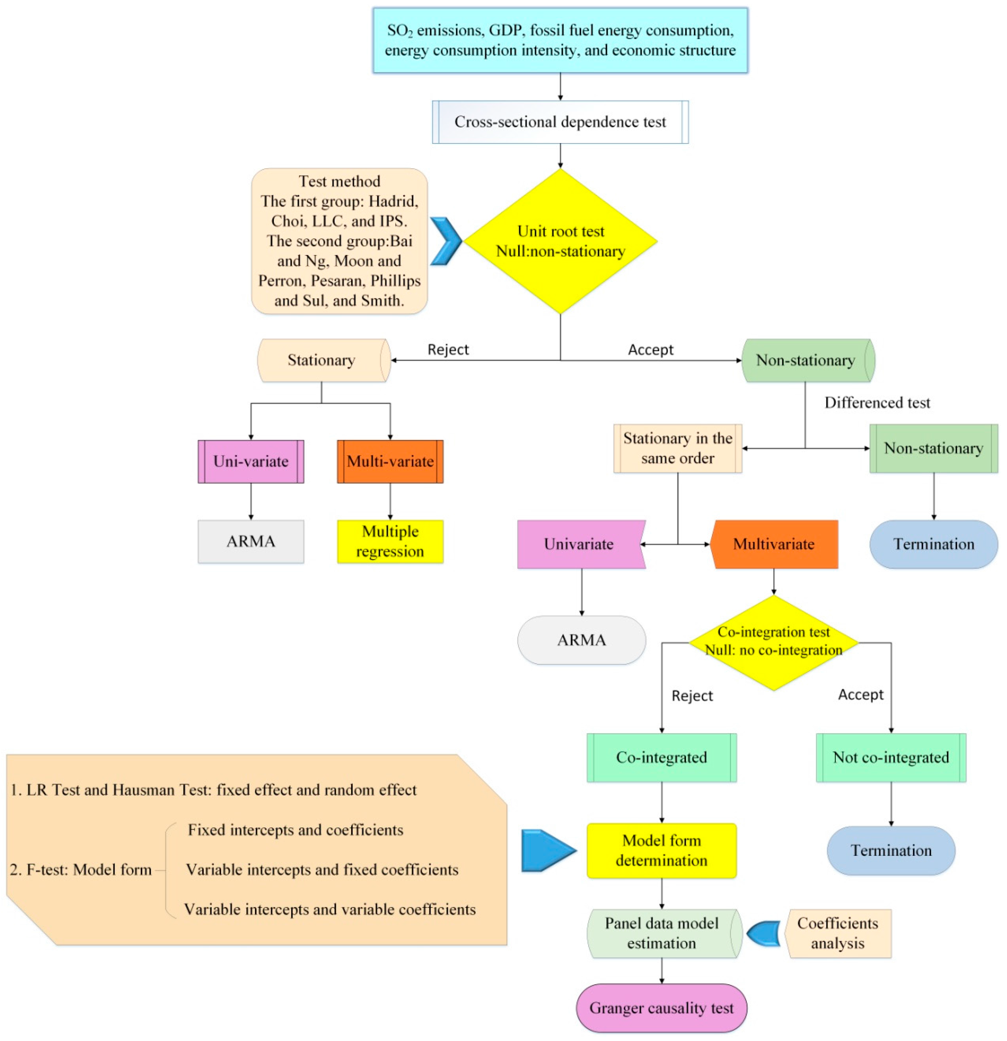
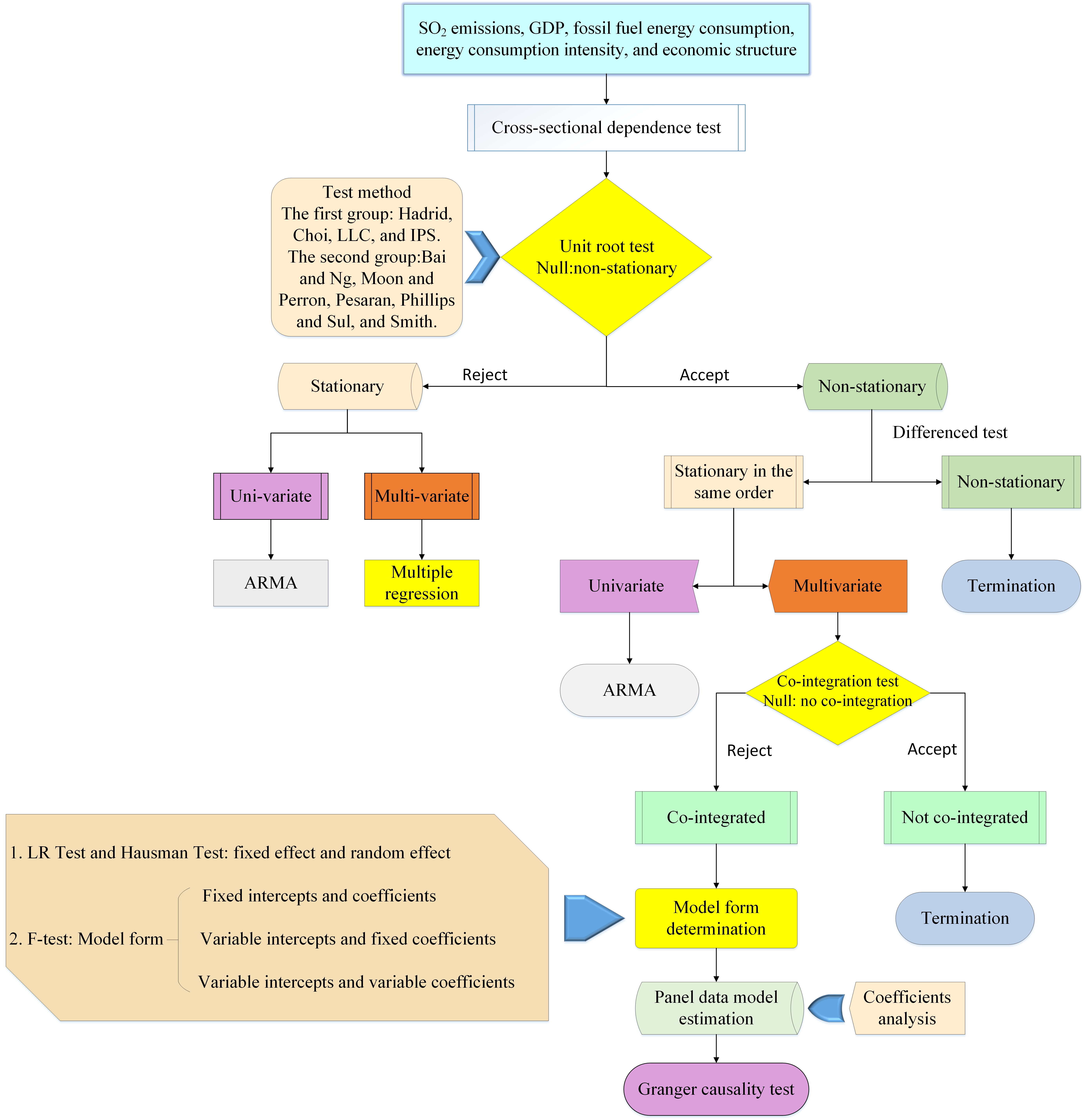
2.6. Theoretical Framework

The theoretical framework is demonstrated in Figure 1. The empirical analysis can be proceeded with following steps.

Step 1: Test for cross-sectional dependence

The empirical analysis will start with cross-sectional dependence test to identify the methods used in unit root test and panel co-integration test.

Step 2: Test for panel unit root

After confirming whether it is necessary to consider cross-sectional dependence, the stable of all variables need to be examined and the methods used in this stage depend on the results of step 1. Only if all variables are stable in the same order, the empirical analysis can proceed to co-integration test.

Step 3: Test for panel co-integration

After verifying all variables are stationary at the same order, Pedroni co-integration examination method will be used for testing whether there exists long-term relationship among SO₂ emissions and all independent variables. If not, the panel data model cannot be established, otherwise, we need to determine the form of panel data model.

Step 4: Test for panel data model form

At this step, LR test and Hausman test are used to determine the fixed effect or random effect of panel data model. And then F-test will be employed to judge whether the panel data model is constant intercepts and coefficients model, the variable intercepts and invariable coefficients model, or the changed intercepts and coefficients model. After identifying the model form, the panel data model can be estimated.

Step 5: Test for Granger causal relationship

At the aim of further and better understanding the relationship among SO₂ emissions, GDP, fossil fuel energy consumption, energy consumption intensity, and economic structure, Granger causality examination method will be used to explore the nexus among these variables. And the direction of causal nexus can provide policy making references for policy makers.

3. Data Sources and Pre-Analysis

3.1. Study Area and Data Sources

At the aim of exploring the contributions of various socio-economic factors to SO₂ discharge and specifically carrying out policy recommendations to reduce SO₂ emissions, this paper investigates the contributions of economic development, fossil fuel energy consumption, energy consuming intensity, and economic structure to SO₂ discharge using the data of five provinces with the highest SO₂ emissions in China during the period of 2002–2015. The provinces selected in this paper are Hebei, Henan, Inner Mongolia, Shandong, and Shanxi.

For economic development, gross domestic production (GDP) is selected to represent the growth of economy, and is converted to the constant price using 2002 as basic period. For fossil fuel energy consumption, it is made up of the use amount of coal, crude oil, and natural gas. The statistical unit is 10⁴ ton for coal and crude oil consumption, and 10⁸ cubic meter (m³) for natural gas consumption. On the purpose of maintaining consistency of statistical requirements, the consumption units are converted to 10⁴ ton coal equivalent (tce) employing the coefficients suggested in the China Energy Statistic Yearbook, which are 0.7143 tce/t, 1.4286 tce/t, and 1.33 tce/10³ m³ for the consuming of coal, crude oil, and natural gas [48,49,50,51,52,53,54,55,56,57,58,59,60,61,62,63,64,65,66,67]. For energy consuming intensity, it is represented by the value of energy consumption for the whole society divided by GDP (constant price taking 2002 as basic period). For economic structure, it is expressed by the value of the added value for secondary industry divided by GDP due to the high proportion of added value of secondary industry in GDP. All data of the variables mentioned above as well as the data of SO₂ emissions are collected from the official website of National Statistics Bureau of China. This dataset on SO₂ emissions in provincial level allowed this research from provincial aspects over a long period.

The representation forms of all independent variables and SO₂ discharge used in the panel data model are listed in

Table 1. The representation forms of all variables in panel data model.

Variables	Definition	Unit
SO2	The amount of sulfur dioxide emissions	Thousand tons
GDP	The development of economy	Billion yuan
FEC	The amount of fossil fuel energy consumption	Million tce
ECI	Energy consumption intensity for the whole society	Tce/million yuan
ES	The proportion of secondary industry added value accounted for GDP	%

. The data of SO₂ discharge, GDP, fossil fuel energy consumption, and energy consuming intensity are transformed into natural logarithmic form. The data of the economic structure is multiplied by 100 before being converted into the natural logarithmic form.

3.2. Pre-Analysis

Since the high level of SO₂ discharge can cause acid rain weather which seriously damage to human health, it is necessary to research on the contributions of significant socio-economic factors on SO₂ emissions to provide references for policy makers. Figure 2 displays the spatial distribution of SO₂ discharge in 32 primary provinces of China in the year of 2010 and 2015. As can be seen from the figure, the SO₂ emissions amount of Inner Mongolia, Shanxi, Hebei, Shandong, Henan, Sichuan, and Guizhou in 2010 were more than 1100 thousand tons, which contributed more than 40% of SO₂ emissions in China. During the period of 2011–2015, the SO₂ emissions amount of most provinces showed downward trend. However, the amount of SO₂ discharge in Hebei, Henan, Inner Mongolia, Shandong, and Shanxi still maintained more than 1100 thousand tons, among which Shandong ranked the first with 1525.67 thousand tons and Hebei ranked the fifth with 1108.37 thousand tons. Therefore, these five provinces are selected to be the objects of this study aiming at better understanding the relationships between SO₂ emissions and significant socio-economic indicators in these five provinces.

The development trend of GDP for the selected five provinces from 2002 to 2015 is demonstrated in Figure 3. As indicated in the figure, the economy scale of Shandong ranks the first, with 1027.55 billion yuan in 2002 and 4486.34 billion yuan in 2015. Before 2009, the scale of economic development in Hebei and Henan was close to each other, while after 2009, the growth rate of Hebei lagged behind Henan. The economic scales of Inner Mongolia and Shanxi are much smaller than other three provinces, with 194.09 billion yuan for Inner Mongolia and 232.48 billion yuan for Shanxi in 2002, and 1226.40 billion yuan and 856.93 billion yuan for Inner Mongolia and Shanxi in 2015, respectively.

The development tendency of fossil fuel energy consumption from 2002 to 2015 for the chosen five provinces is indicated in Figure 4. With the largest economic scale, the fossil fuel energy consumption of Shandong also ranked the first with 495.34 million tce in 2015 and 10.28% annual growth rate. Although the economic scale of Shanxi ranked the fifth, the fossil fuel energy consumption of it ranked the second with 378.68 million tce in 2015, which means the development of economy in Shanxi mainly depends on the consumption of fossil fuel energy. The amount of fossil fuel energy consumption in Inner Mongolia increased fast from 69.90 million tce in 2002 to 368.83 million tce in 2015 with 14.14% annual growth rate ranking the third. The fossil fuel energy consumption of Hebei and Henan showed a downtrend from 323.57 million tce for Hebei and 292.49 million tce for Henan in 2011 to 306.10 million tce for Hebei and 245.67 million tce for Henan in 2015.

The development trend of energy consuming intensity from 2002 to 2015 for five provinces is illustrated in Figure 5. As depicted in the figure, the energy consuming intensity of Hebei, Henan, Inner Mongolia, Shandong and Shanxi all showed decrease tendency from 2002 to 2015. Based on the analysis of GDP and fossil fuel energy consumption, we can conclude that the energy use efficiency of Shanxi was the lowest, thus the energy consuming intensity of Shanxi should be the highest. It can also be obtained from the figure that the energy consuming intensity of Shanxi ranked the first which is much higher than other four provinces.

The development tendency of economic structure for the selected five provinces from 2002 to 2015 is implied in Figure 6. As displayed in the figure, at the beginning of the analysis phase, the proportion of secondary industry added value accounted for GDP in Shandong was the highest with 50.46%, and then it reduced to 46.80% in 2015 ranking the fourth. The proportion of secondary industry added value accounted for GDP in Shanxi ranked the second in 2002, and then it decreased to 40.69% in 2015 ranking the fifth. The proportion of secondary industry added value accounted for GDP in Inner Mongolia, Henan and Hebei first increased to 55.97% in 2011, 57.28% in 2010, and 54.34% in 2008, and then dropped to 50.48%, 48.42%, and 48.27% in 2015.

4. Empirical Analysis

4.1. Results for Cross-Sectional Dependence Examination

The initial stage of empirical analysis should be cross-sectional dependence examination which decides the methods selected to test unit root. The results of Pesaran cross-sectional dependence examination method utilized in this study are shown in

Table 2. Results for cross-sectional dependence test.

Cross-Sectional Dependence Test	Pesaran’s Test of Cross-Sectional Independence	p-Value
Pesaran cross-sectional dependence test	3.8687	0.0147 b

Notes: The probability values less than the confidence level demonstrates the null hypothesis is rejected. ^b demonstrates 5% significance level.

. As can be seen from p-value in Table 2, the null hypothesis can be rejected at 5% confidence level. Therefore, the methods employed to test data stationary and co-integration relationship should take cross-sectional dependence into consideration.

4.2. Results for Unit Root Examination

Since the following analysis should take cross-sectional dependence into consideration, at the stage of testing data series stationary, L.L&C, IPS, Augmented Dickey Fuller-Fisher (ADF-Fisher) and Phillips-Perron Fisher (PP-Fisher) examination approaches are selected. As shown in

Table 3. Results for panel unit root test.

Form	Variables	L.L&C	IPS	ADF-Fisher	PP-Fisher	Conclusions
Level	lnSO2	0.86482	0.40240	0.78035	1.50630	Non-stationary
		(0.8064)	(0.6563)	(0.6769)	(0.4709)
	lnGDP	0.63442	2.02464	0.03046	0.00020	Non-stationary
		(0.7371)	(0.9785)	(0.9849)	(0.9999)
	lnFEC	−1.05854	−0.29416	2.03733	1.33161	Non-stationary
		(0.1449)	(0.3843)	(0.3611)	(0.5139)
	lnECI	1.45960	2.51124	0.01416	0.00313	Non-stationary
		(0.9278)	(0.9940)	(0.9929)	(0.9984)
	lnES	3.47883	1.85937	0.06078	0.19242	Non-stationary
		(0.9997)	(0.9685)	(0.9701)	(0.9083)
First Differences	ΔlnSO2	−2.01509	−1.52874	5.66558	6.09979	Stationary
		(0.0219) b	(0.0432) b	(0.0488) b	(0.0474) b
	ΔlnGDP	−3.88122	−1.98857	7.21690	15.1666	Stationary
		(0.0001) a	(0.0234) b	(0.0271) b	(0.0005) a
	ΔlnFEC	−2.87180	−2.46566	8.46117	14.4327	Stationary
		(0.0020) a	(0.0014) a	(0.0252) b	(0.0109) b
	ΔlnECI	−3.87144	−2.52606	8.84465	13.1489	Stationary
		(0.0001) a	(0.0058) a	(0.0120) b	(0.0014) a
	ΔlnES	−2.24266	−2.01695	7.59160	8.75067	Stationary
		(0.0125) b	(0.0219) b	(0.0225) b	(0.0126) b

Notes: probability values are listed in the brackets. The probability values less than the confidence level demonstrates the variable is stationary. ^a illustrates 1% significance level; ^b demonstrates 5% significance level.

, regarding to the probability values in the brackets of different examination methods for variables, we can obtain that all variables are not stable in their level form. Then all variables need to be differenced. ΔlnSO₂, ΔlnGDP, ΔlnFEC, ΔlnECI, and ΔlnES are utilized to represent the first difference form for SO₂ emissions, GDP, fossil fuel energy consumption, energy consumption intensity, and economic structure in natural logarithmic form. Since all of the probability values in brackets are less than the confidence level, SO₂ emissions and four independent variables are stable in the same order.

4.3. Results for Panel Co-Integration Examination

As all variables are first order differential stationary, the empirical analysis can step to panel co-integration test. Pedroni’s co-integration examination approach is utilized in this stage and the statistic values of it are illustrated in

Table 4. Results for panel co-integration test.

Test Method	Test Statistics	Value	Probability
Pedroni	Panel v-Statistic	−1.845422	0.0479 b
	Panel rho-Statistic	−1.025375	0.0410 b
	Panel PP-Statistic	−7.517128	0.0000 a
	Panel ADF-Statistic	−1.990137	0.0211 b
	Group rho-Statistic	−1.937089	0.0126 b
	Group PP-Statistic	−8.544697	0.0000 a
	Group ADF-Statistic	−1.536537	0.0295 b

Notes: ^a points to 1% level of confidence; ^b refers to 5% confidence level.

. Since all values of probability are less than the confidence level, it can be verified that the long-term co-integration relationship is existed among SO₂ discharge, GDP, fossil fuel energy consumption, energy consumption intensity, and economic structure.

4.4. Model Form Determination

As there exists long-run co-integration relationship among all variables, the empirical analysis can proceed to model estimation. First, the effect of panel data model needs to be identified. Generally, LR test and Hausman test are used to determine whether the panel data model is fixed effect or random effect. The test results are shown in

Table 5. Results for panel data model effect test.

LR Test Results
		Statistic	Prob.
Cross-section F		14.382367	0.0001 a
Hausman Test Results
	Chi-Square Statistic		Prob.
Cross-Section Random	38.453127		0.0000 a
Variable	Fixed	Random	Var(Diff.)	Prob.
GDP	1.472034	1.142088	0.023867	0.0000 a
FEC	1.503979	0.505360	0.027417	0.0015 a
ECI	−1.309788	0.034978	0.003147	0.0027 a
ES	0.976341	0.736415	0.004137	0.0059 a

Notes: ^a refers to 1% significance level.

. With regard to LR examination approach, the probability value is less than the significance level, which implies that the panel data model should be fixed effect. As for Hausman examination results, based on the value of cross-section random and probability values of all independent variables, it is verified that the panel data model should be fixed effect.

Then the panel data model form of the unchanged intercepts and coefficients model, the changed intercepts and unchanged coefficients model, and the changed intercepts and coefficients model need to be determined employing F-test. Firstly, we need to obtain three sum square residual values represented by S₁, S₂, and S₃ of Equations (11)–(13), respectively. Secondly, we can calculate the values of F₁ and F₂ statistics based on Equations (14) and (15). Thirdly, the panel data model form can be confirmed. If the value of F₂ is smaller than the critical value F_2,α((N − 1)(K + 1),(NT − N(K + 1)), the panel data model is confirmed to be the model with constant intercepts and coefficients, if not, the hypothesis H₁ will be examined. If the value of F₁ is larger than the critical value F_1,α((N − 1)K,(NT − N(K + 1)), the panel data model is verified to be the model with changed intercepts and coefficients, if not, it is judged to be the model with variable intercepts and invariable coefficients. In accordance with the results for F-test, both of the values of F₁ and F₂ statistics are more than the critical values at the given significance level. Therefore, the established panel data model should be the changed intercepts and coefficients model as

Table 6. Results for F-test.

S1	S2	S3	F1	F2
0.021035	0.057892	0.090373	4.927992	7.416710

shown.

4.5. Estimation for Panel Data Model and Provincial Comparative Analysis

Based on the above examination process, a fixed effect panel data model with changed intercepts and coefficients consists of SO₂ discharge, GDP, fossil fuel energy consumption, energy consumption intensity, and economic structure can be established for Hebei, Henan, Inner Mongolia, Shandong, and Shanxi. The estimated coefficients of the panel data model and the test results for the effectiveness of the model are listed in

Table 7. The estimated results for panel data model.

Variables	Hebei	Henan	Inner Mongolia	Shandong	Shanxi
lnGDP	0.6314	0.6525	0.6198	0.7378	0.5928
	(0.0368) b	(0.0075) a	(0.0332) b	(0.0023) a	(0.0022) a
lnFEC	0.8894	0.8039	0.8767	0.9312	0.8905
	(0.0042) a	(0.0250) b	(0.0451) b	(0.0089) a	(0.0004) a
lnECI	0.3907	0.3885	0.4103	0.4331	0.3098
	(0.0423) b	(0.0413) b	(0.0399) b	(0.0385) b	(0.0275) b
lnES	0.4488	0.4425	0.4523	0.4828	0.3364
	(0.0469) b	(0.0421) b	(0.0327) b	(0.0069) a	(0.0016) a
C	1.0691	2.5034	1.0053	4.0775	3.6094
R2	0.9981	F-statistic	129.0515	Prob	0.0000

Notes: probability values are listed in the brackets. The values of the probability smaller than the specific confidence level demonstrates the coefficients are significant. ^a refers to 1% confidence level; ^b points to 5% confidence level.

. The value of R² is 0.9981 which means the fitting effect of the model is pretty good. The value of F-statistic is 129.0515, which is much more than the critical value representing the coefficients of the model are all significant. Therefore, it can be confirmed that the established panel data model is valid and significant.

As all variables are converted to logarithmic form, the coefficients represent elasticities. Through analyzing the coefficients, we can conclude that:

(1)

Compared with GDP, energy consumption intensity, and economic structure, fossil fuel energy consumption makes the greatest contribution to SO₂ discharge. Since fossil fuel energy contain large amount of sulfur element, the combustion of fossil fuel energy will release a great deal of sulfide which is the main source of sulfur dioxide. Through comparing the different contributions of fossil fuel energy consumption to SO₂ emissions for different provinces, it can be summarized that the more the fossil fuel energy consumption, the greater the contribution made by it to SO₂ emissions. Since the fossil fuel energy consumption amount of Shandong ranked the first, the contribution of fossil fuel energy consumption to SO₂ emissions is the greatest, followed by Shanxi. The contribution of fossil fuel energy consumption to SO₂ emissions in Henan is the smallest.

(2)

The contribution of GDP to SO₂ emissions is less than fossil fuel energy consumption, but more than energy consumption intensity and economic structure. Compared with the contribution of fossil fuel energy consumption to SO₂ emissions, GDP make much less contribution to SO₂ emissions. Through comparing the different devotions of GDP to SO₂ emissions among five selected provinces, it can be concluded that the larger the scale of the economy, the greater the devotion made by it to SO₂ emissions. Since the economy scale of Shandong ranked the first, the devotion of GDP to SO₂ emissions in Shandong is the greatest, followed by Henan. GDP in Shanxi contributes the smallest to SO₂ emissions.

(3)

The more the proportion of the secondary industry added value accounted in GDP, the greater the contribution of the economic structure and energy consumption intensity to SO₂ emissions. From the overall trend of the proportion for secondary industry added value accounted in GDP, the proportions of secondary industry added value accounted in GDP for Shandong and Inner Mongolia are higher than other three provinces, and the contributions of energy consumption intensity and economic structure to SO₂ emissions of Shandong and Inner Mongolia are higher than Hebei, Henan, and Shanxi.

4.6. Analysis for Granger Causality Relationship

The results of Granger causality test for the established panel data model are listed in

Table 8. Results for Granger causality examination.

Null Hypothesis	Hebei	Henan	Inner Mongolia	Shandong	Shanxi
LnGDP does not Granger cause lnSO2	13.9091	5.6767	13.8430	4.1553	4.9914
	(0.0036) a	(0.0343) b	(0.0037) a	(0.0463) b	(0.0450) b
LnSO2 does not Granger cause LnGDP	2.24072	0.1902	1.1868	0.1243	0.0970
	(0.1770)	(0.8309)	(0.1037)	(0.8851)	(0.1987)
LnFEC does not Granger cause lnSO2	11.6568	7.0617	5.0697	12.8058	6.3492
	(0.0376) b	(0.0209) b	(0.0464) b	(0.0274) b	(0.0268) b
LnSO2 does not Granger cause LnFEC	5.04149	6.4067	5.0836	4.2632	5.8372
	(0.0496) b	(0.0306) b	(0.0207) b	(0.0159) b	(0.0221) b
LnECI does not Granger cause lnSO2	8.2239	5.6432	6.3869	5.7609	4.9374
	(0.0426) b	(0.0347) b	(0.0264) b	(0.0402) b	(0.0214) b
LnSO2 does not Granger cause LnECI	2.93488	2.0607	2.4265	0.4482	1.0361
	(0.1187)	(0.1978)	(0.1583)	(0.6559)	(0.4035)
LnES does not Granger cause lnSO2	11.0065	9.5477	26.6237	5.5607	4.8368
	(0.0129) b	(0.0113) b	(0.0005) a	(0.0256) b	(0.0252) b
LnSO2 does not Granger cause LnES	1.2259	1.5802	1.3166	0.1397	0.1608
	(0.3496)	(0.2714)	(0.1028)	(0.8720)	(0.8545)

Notes: probability values are listed in the brackets. ^a points to 1% confidence level; ^b refers to 5% confidence level.

. If the probability values in brackets are less than the specific significance level, there exists Granger causality relationship between these two variables. As illustrated in Table 8, we can summarize that:

(1)

For the selected five provinces, there exists a bi-directional causality relationship between fossil fuel energy consumption and SO₂ emissions. This indicates that the decrease of fossil fuel energy consumption can contribute to the reduction of SO₂ emissions, while the decrease of SO₂ emissions will have a negative impact on fossil fuel energy consumption.

(2)

There exist uni-directional causal relationships running from GDP to SO₂ emissions, from energy consumption intensity to SO₂ emissions, and from economic structure to SO₂ emissions. That means the increase of GDP will lead to the raise of SO₂ emissions, the decrease of energy consumption intensity will bring about the decline of SO₂ emissions, and the decrease of the proportion for the secondary industry added value accounted in GDP will result in the reduction of SO₂ emissions. But there is no feedback from SO₂ emissions to GDP, energy consumption intensity, and economic structure.

5. Conclusions and Policy Implications

This paper investigated the relationship among SO₂ emissions, GDP, fossil fuel energy consumption, energy consumption intensity, and economic structure of five provinces in China with the highest SO₂ emissions employing panel data model approach spanning from 2002 to 2015. Based on panel unit root examination to confirm all variables are stable in the same order, panel co-integration examination to verify all variables are co-integrated in the long-term, and model form determination tests, the panel data model can be estimated and the Granger causality examination can be conducted, which provided strong evidence on the complicated relationships among these variables. Through analyzing the established panel data model, the main conclusions are as follows:

(1)

Fossil fuel energy consumption makes the greatest contribution to SO₂ discharge compared with GDP, energy consumption intensity, and economic structure. And the more the fossil fuel energy consumption, the greater the devotion made by it to SO₂ emissions.

(2)

GDP makes less contribution to SO₂ emissions than fossil fuel energy consumption, and the larger the scale of the economy, the greater the contribution made by it to SO₂ emissions.

(3)

The higher the proportion of the secondary industry added value accounted in GDP, the more the devotion made by the economic structure and energy consumption intensity to SO₂ emissions.

Through investigating the causal relationship among SO₂ emissions, GDP, fossil fuel energy consumption, energy consumption intensity, and economic structure of Hebei, Henan, Inner Mongolia, Shandong, and Shanxi using Granger causality examination method, we can obtain that:

(1)

A bi-directional causal relationship exists between fossil fuel energy consumption and SO₂ emissions among five selected provinces.

(2)

Uni-directional causal nexus exist running from GDP to SO₂ emissions, from energy consumption intensity to SO₂ emissions, and from economic structure to SO₂ emissions among five chosen provinces.

The empirical analysis of this research can make policy makers better understand the complex relationships between SO₂ emissions, GDP, fossil fuel energy consumption, energy consumption intensity, and economic structure of Hebei, Henan, Inner Mongolia, Shandong, and Shanxi. In this way, the significant influencing factors of SO₂ discharge can be found, and effective and practicable policies can be formulated according to the contributions of different factors and causality relationships. Therefore, regarding to the above econometric analysis, the following recommendations are put forward:

(1)

Giving full play to the guiding role of price signals, and improving the price policy for desulfurization. Based on the empirical analysis, it can be found that the consumption of fossil fuel energy makes the greatest contribution to SO₂ emissions. However, in the long-run, energy consumption of various provinces in China will still depend on fossil fuel energy to a large extent. Therefore, in the process of using fossil fuel energy, desulfurization equipment is needed to reduce sulfur emissions. Considering about the increase of the cost for enterprises using desulfurization equipment, it is necessary to implement a certain price subsidy policy so that the increased cost due to the use of desulfurization technique can be covered, which can also encourage enterprises to develop desulfurization technology.

(2)

Formulating a new comprehensive evaluation indicator to measure the regional development level considering economic development and environmental impacts. Currently, GDP is deemed as the significant indicator to evaluate the regional development level, which neglects the environmental impact. Therefore, it is essential to establish a comprehensive evaluation system for measuring regional development level, which can not only consider the level of economic development, but also take the impact of pollutant emissions on the environment in the process of rapid economic development into consideration.

(3)

Exploring renewable and sustainable energy sources to substitute for fossil fuel energy. Considering the high pollution and limited nature of fossil fuel energy, we should actively exploit other renewable energy to take over the use of fossil resources. Based on regional resources endowment, people in inland areas should energetically develop the use of wind energy and solar energy, such as Hebei, Henan, Inner Mongolia, and Shanxi, while people in coastal areas should positively explore the use of hydropower and tidal energy, such as Shandong.

(4)

Developing high value added and low pollution emissions industries and reducing the proportion of secondary industry. According to the empirical analysis, we can obtain that the higher the proportion of the secondary industry accounted in GDP, the more the devotion made by the economic structure and energy consumption intensity to SO₂ emissions. Therefore, policy makers should draft related policies for economic structure adjustment, which should aims at reducing the proportion of secondary industry and developing high value added and low pollution emissions industries. Additionally, policies related to improve energy using efficiency should be executed.

Based on the above analysis, although the results of this study are inspiring, we also have lots of work needed to be done in the future. The policy effect of reducing SO₂ emissions should be quantified and added to the panel data model to analyze the function of policies in decreasing SO₂ discharge. Additionally, it is also necessary to analyze the influence of renewable energy and its relevant policies on SO₂ emissions. Therefore, policymakers can grasp the policy effect, and propose more effective policies and measures.

References

1. Zhu, L.; Gan, Q.; Liu, Y.; Yan, Z. The impact of foreign direct investment on SO2 emissions in the Beijing-Tianjin-Hebei region: A spatial econometric analysis. J. Clean. Prod. 2017, 166, 189–196. [Google Scholar] [CrossRef]
2. Wang, H.; An, J.; Shen, L.; Zhu, B.; Pan, C.; Liu, Z.; Liu, X.; Duan, Q.; Liu, X.; Wang, Y. Mechanism for the formation and microphysical characteristics of submicron aerosol during heavy haze pollution episode in the Yangtze River Delta, China. Sci. Total Environ. 2014, 490, 501–508. [Google Scholar] [CrossRef] [PubMed]
3. Wang, Y.; Ying, Q.; Hu, J.; Zhang, H. Spatial and temporal variations of six criteria air pollutants in 31 provincial capital cities in China during 2013–2014. Environ. Int. 2014, 73, 413–422. [Google Scholar] [CrossRef] [PubMed]
4. Hsu, A. 2016 Environmental Performance Index; Yale University: New Haven, CT, USA, 2016. [Google Scholar]
5. Qu, Y.; An, J.; He, Y.; Zheng, J. An overview of emissions of SO2 and NOx and the long-range transport of oxidized sulfur and nitrogen pollutants in East Asia. J. Environ. Sci. 2016, 44, 13–25. [Google Scholar] [CrossRef] [PubMed]
6. Zhang, H.; Wang, Z.; Zhang, W. Exploring spatiotemporal patterns of PM2.5 in China based on ground-level observations for 190 cities. Environ. Pollut. 2016, 216, 559–567. [Google Scholar] [CrossRef] [PubMed]
7. Zhou, Z.; Ye, X.; Ge, X. The Impacts of Technical Progress on Sulfur Dioxide Kuznets Curve in China: A Spatial Panel Data Approach. Sustainability 2017, 9, 674. [Google Scholar] [CrossRef]
8. Sinha, A. Trilateral association between SO2/NO2 emission, inequality in energy intensity, and economic growth: A case of Indian cities. Atmos. Pollut. Res. 2016, 7, 647–658. [Google Scholar] [CrossRef]
9. Yao, L.; Liu, J.; Zhou, T.; Wang, R. An analysis of the driving forces behind pollutant emission reduction in Chinese industry. J. Clean. Prod. 2016, 112, 1395–1400. [Google Scholar] [CrossRef]
10. Han, Y.; Xiong, X.; Liu, Y.; Pan, Y.R.; Zhang, Y.B. The Analysis of Factors Affecting SO2 Emission of Chinese Industry. In Proceedings of the 2011 International Conference on Computer and Management (CAMAN), Wuhan, China, 19–21 May 2011; pp. 1–11. [Google Scholar]
11. Wang, Q.; Wang, Y.; Zhou, P.; Wei, H. Whole process decomposition of energy-related SO2 in Jiangsu Province, China. Appl. Energy 2017, 194, 679–687. [Google Scholar] [CrossRef]
12. Yang, X.; Wang, S.; Zhang, W.; Li, J.; Zou, Y. Impacts of energy consumption, energy structure, and treatment technology on SO2 emissions: A multi-scale LMDI decomposition analysis in China. Appl. Energy 2016, 184, 714–726. [Google Scholar] [CrossRef]
13. Grossman, G.M.; Krueger, A.B. Economic growth and the environment. Q. J. Econ. 1995, 110, 353–377. [Google Scholar] [CrossRef]
14. Holtz-Eakin, D.; Selden, T.M. Stoking the fires? CO2 emissions and economic growth. J. Public Econ. 1995, 57, 85–101. [Google Scholar] [CrossRef]
15. Stern, D.I.; Common, M.S.; Barbier, E.B. Economic growth and environmental degradation: The environmental Kuznets curve and sustainable development. World Dev. 1996, 24, 1151–1160. [Google Scholar] [CrossRef]
16. Kaufmann, R.K.; Davidsdottir, B.; Garnham, S.; Pauly, P. The determinants of atmospheric SO2 concentrations: Reconsidering the environmental Kuznets curve. Ecol. Econ. 1998, 25, 209–220. [Google Scholar] [CrossRef]
17. List, J.A.; Gallet, C.A. The environmental Kuznets curve: Does one size fit all? Ecol. Econ. 1999, 31, 409–423. [Google Scholar] [CrossRef]
18. Selden, T.M.; Song, D. Environmental quality and development: Is there a Kuznets curve for air pollution emissions? J. Environ. Econ. Manag. 1994, 27, 147–162. [Google Scholar] [CrossRef]
19. Harbaugh, W.T.; Levinson, A.; Wilson, D.M. Reexamining the empirical evidence for an environmental Kuznets curve. Rev. Econ. Stat. 2002, 84, 541–551. [Google Scholar] [CrossRef]
20. Miah, M.D.; Masum, M.F.; Koike, M. Global observation of EKC hypothesis for CO2, SOx and NOx emission: A policy understanding for climate change mitigation in Bangladesh. Energy Policy 2010, 38, 4643–4651. [Google Scholar] [CrossRef]
21. Menegaki, A.N.; Tsagarakis, K.P. Rich enough to go renewable, but too early to leave fossil energy? Renew. Sustain. Energy Rev. 2015, 41, 1465–1477. [Google Scholar] [CrossRef]
22. Stern, D.I.; Common, M.S. Is there an environmental Kuznets curve for sulfur? J. Environ. Econ. Manag. 2001, 41, 162–178. [Google Scholar] [CrossRef]
23. Junyi, S.H. A simultaneous estimation of environmental Kuznets curve: Evidence from China. China Econ. Rev. 2006, 17, 383–394. [Google Scholar]
24. Fodha, M.; Zaghdoud, O. Economic growth and pollutant emissions in Tunisia: An empirical analysis of the environmental Kuznets curve. Energy Policy 2010, 38, 1150–1156. [Google Scholar] [CrossRef]
25. Stern, D.I. The rise and fall of the environmental Kuznets curve. World Dev. 2004, 32, 1419–1439. [Google Scholar] [CrossRef]
26. Kohler, M. CO2 emissions, energy consumption, income and foreign trade: A South African perspective. Energy Policy 2013, 63, 1042–1050. [Google Scholar] [CrossRef]
27. Shahbaz, M.; Uddin, G.S.; Rehman, I.U.; Imran, K. Industrialization, electricity consumption and CO2 emissions in Bangladesh. Renew. Sustain. Energy Rev. 2014, 31, 575–586. [Google Scholar] [CrossRef]
28. Wang, Y.; Han, R.; Kubota, J. Is there an environmental Kuznets curve for SO2 emissions? A semi-parametric panel data analysis for China. Renew. Sustain. Energy Rev. 2016, 54, 1182–1188. [Google Scholar] [CrossRef]
29. Shafik, N.; Bandyopadhyay, S. Economic Growth and Environmental Quality: Time-Series and Cross-Country Evidence; World Bank: Washington, DC, USA, 1992. [Google Scholar]
30. Unruh, G.C.; Moomaw, W.R. An alternative analysis of apparent EKC-type transitions. Ecol. Econ. 1998, 25, 221–229. [Google Scholar] [CrossRef]
31. Stern, D.I. Progress on the environmental Kuznets curve? Environ. Dev. Econ. 1998, 3, 173–196. [Google Scholar] [CrossRef]
32. Pesaran, M.H. General Diagnostic Tests for Cross Section Dependence in Panels; CESifo Working Papers No. 1233; CESifo: München, Germany, 2004; pp. 255–260. [Google Scholar]
33. Breusch, T.S.; Pagan, A.R. The Lagrange multiplier test and its applications to model specification in econometrics. Rev. Econ. Stud. 1980, 47, 239–253. [Google Scholar] [CrossRef]
34. Hadri, K. Testing for stationarity in heterogeneous panel data. Econom. J. 2000, 3, 148–161. [Google Scholar] [CrossRef]
35. Choi, I. Unit root tests for panel data. J. Int. Money Financ. 2001, 20, 249–272. [Google Scholar] [CrossRef]
36. Levin, A.; Lin, C.F.; Chu, C.S.J. Unit root tests in panel data: Asymptotic and finite-sample properties. J. Econom. 2002, 108, 1–24. [Google Scholar] [CrossRef]
37. Im, K.S.; Pesaran, M.H.; Shin, Y. Testing for unit roots in heterogeneous panels. J. Econom. 2003, 115, 53–74. [Google Scholar] [CrossRef]
38. Bai, J.; Ng, S. A PANIC attack on unit roots and cointegration. Econometrica 2004, 72, 1127–1177. [Google Scholar] [CrossRef]
39. Moon, H.R.; Perron, B. Testing for a unit root in panels with dynamic factors. J. Econom. 2004, 122, 81–126. [Google Scholar] [CrossRef]
40. Pesaran, M.H. A simple panel unit root test in the presence of cross-section dependence. J. Appl. Econom. 2007, 22, 265–312. [Google Scholar] [CrossRef]
41. Phillips, P.C.B.; Sul, D. Dynamic panel estimation and homogeneity testing under cross section dependence. Econom. J. 2003, 6, 217–259. [Google Scholar] [CrossRef]
42. Smith, L.V.; Leybourne, S.; Kim, T.H.; Newbold, P. More powerful panel data unit root tests with an application to mean reversion in real exchange rates. J. Appl. Econom. 2004, 19, 147–170. [Google Scholar] [CrossRef]
43. Pedroni, P. Panel Cointegration: A Symptotic and Finite Sample Properties of Pooled Time Series Tests with an Application to the PPP Hypothesis. Econ. Theory 2004, 20, 597–625. [Google Scholar] [CrossRef]
44. Ou, J.; Liu, X.; Li, X.; Chen, Y. Quantifying the relationship between urban forms and carbon emissions using panel data analysis. Landsc. Ecol. 2013, 28, 1889–1907. [Google Scholar] [CrossRef]
45. Wang, S.; Fang, C.; Wang, Y.; Huang, Y.; Ma, H. Quantifying the relationship between urban development intensity and carbon dioxide emissions using a panel data analysis. Ecol. Indic. 2015, 49, 121–131. [Google Scholar] [CrossRef]
46. Engle, R.F.; Granger, C.W.J. Co-integration and error correction: Representation, estimation, and testing. Econometrica 1987, 55, 251–276. [Google Scholar] [CrossRef]
47. Granger, C.W.J. Investigating causal relations by econometric models and cross-spectral methods. Econom. Econom. 1969, 37, 424–438. [Google Scholar] [CrossRef]
48. National Bureau of Statistics of China. China Energy Statistical Yearbook 1996; China Statistics Press: Beijing, China, 1996.
49. National Bureau of Statistics of China. China Energy Statistical Yearbook 1997; China Statistics Press: Beijing, China, 1997.
50. National Bureau of Statistics of China. China Energy Statistical Yearbook 1998; China Statistics Press: Beijing, China, 1998.
51. National Bureau of Statistics of China. China Energy Statistical Yearbook 1999; China Statistics Press: Beijing, China, 1999.
52. National Bureau of Statistics of China. China Energy Statistical Yearbook 2000; China Statistics Press: Beijing, China, 2000.
53. National Bureau of Statistics of China. China Energy Statistical Yearbook 2001; China Statistics Press: Beijing, China, 2001.
54. National Bureau of Statistics of China. China Energy Statistical Yearbook 2002; China Statistics Press: Beijing, China, 2002.
55. National Bureau of Statistics of China. China Energy Statistical Yearbook 2003; China Statistics Press: Beijing, China, 2003.
56. National Bureau of Statistics of China. China Energy Statistical Yearbook 2004; China Statistics Press: Beijing, China, 2004.
57. National Bureau of Statistics of China. China Energy Statistical Yearbook 2005; China Statistics Press: Beijing, China, 2005.
58. National Bureau of Statistics of China. China Energy Statistical Yearbook 2006; China Statistics Press: Beijing, China, 2006.
59. National Bureau of Statistics of China. China Energy Statistical Yearbook 2007; China Statistics Press: Beijing, China, 2007.
60. National Bureau of Statistics of China. China Energy Statistical Yearbook 2008; China Statistics Press: Beijing, China, 2008.
61. National Bureau of Statistics of China. China Energy Statistical Yearbook 2009; China Statistics Press: Beijing, China, 2009.
62. National Bureau of Statistics of China. China Energy Statistical Yearbook 2010; China Statistics Press: Beijing, China, 2010.
63. National Bureau of Statistics of China. China Energy Statistical Yearbook 2011; China Statistics Press: Beijing, China, 2011.
64. National Bureau of Statistics of China. China Energy Statistical Yearbook 2012; China Statistics Press: Beijing, China, 2012.
65. National Bureau of Statistics of China. China Energy Statistical Yearbook 2013; China Statistics Press: Beijing, China, 2013.
66. National Bureau of Statistics of China. China Energy Statistical Yearbook 2014; China Statistics Press: Beijing, China, 2014.
67. National Bureau of Statistics of China. China Energy Statistical Yearbook 2015; China Statistics Press: Beijing, China, 2015.
Figure 1. Theoretical framework for researching the relationship among SO2 emissions, GDP, fossil fuel energy consumption, energy consumption intensity, and economic structure.
Sustainability 10 00657 g001
Figure 2. The spatial distribution for SO2 discharge in China in the year of 2010 (A) and 2015 (B). Note: NX for Ningxia, SX for Shaanxi, SHX for Shanxi, HB for Hebei, SD for Shandong, JS for Jiangsu, HEN for Henan, AH for Anhui, HUB for Hubei, ZJ for Zhejiang, CQ for Chongqing, GZ for Guizhou, HUN for Hunan, JX for Jiangxi, FJ for Fujian, GX for Guangxi, GD for Guangdong, TW for Taiwan, and HN for Hainan.
Sustainability 10 00657 g002
Figure 3. The development trend of GDP for these five provinces (Unit: billion yuan).
Sustainability 10 00657 g003
Figure 4. The development tendency of fossil fuel energy consumption for these five provinces (Unit: million tce).
Sustainability 10 00657 g004
Figure 5. The development trend of energy consuming intensity for these five provinces (Unit: tce/million yuan).
Sustainability 10 00657 g005
Figure 6. The development tendency of economic structure for these five provinces (Unit: %).
Sustainability 10 00657 g006