The Shadow Prices of Carbon Emissions in China’s Planting Industry

Abstract

The shadow prices of carbon emissions are essential for assessing emission abatement costs and formulating environmental public policies. By adopting the directional distance function method, this paper studies the shadow prices of carbon emissions caused by three main emission sources from China’s planting industry for a panel of 30 provinces spanning the period 1997–2014. We find that there is considerable regional heterogeneity in the shadow prices, and, of the 30 provinces, 23 are characterized by decreasing trends while only seven are on the rise over time. This implies that there is inefficiency of resource allocation among provinces, and the capacity for abatement increases during the observed period. The results support the following recommendation: It might be worth attempting to bring agriculture in China into line with its emission rights trading scheme, not only to help motivate the reduction of emissions but also to improve resource allocation. Also, policymakers are required to enhance regional cooperation and facilitate carbon-reduction technology transfer, to improve the immaterial production factors’ contribution to planting industry growth.

1. Introduction

Global greenhouse gas (GHG) emissions and associated climate change have been increasing at accelerating rates in recent decades [1,2]. It is widely acknowledged that GHG emissions resulting from anthropogenic sources are the main cause of global warming. According to Climate Change, Agriculture and Food Security (CCAFS), direct emissions from food systems have reached 19–29% of overall emissions caused by human activities [3]. China, meanwhile, as the biggest carbon emitter, produces 28% of the world’s total emissions [2], and its agricultural sector’s emissions, which account for 16–17% of its total [4], are roughly equivalent to 70% of India’s national emissions. Since China announced in the Paris Agreement that it would shoulder its responsibility for curtailing carbon emissions, its agricultural carbon emissions should not be a neglected issue any longer. Therefore, in an effort to come into compliance with China’s “low-carbon economy” regime, it is worth examining the abatement costs of carbon emissions for China’s agricultural sector. The main objective of our paper is to accomplish this empirical work from the perspective of the planting industry, China’s most important, representative agricultural industry. Also, this is fundamental to the design of carbon reduction policies.

As global climate change becomes an increasing worldwide concern, a large number of studies have focused on the issue of GHG emission abatement and the environmental performance of global and regional economies. Since undesirable outputs, such as GHGs, that are by-products of the production process are non-marketable and cannot be priced in accordance with normal commodities, there would be obstacles if the costs to reduce them were to be measured. Extensive studies have been conducted to solve this problem. The shadow price method is one of the most important approaches for deriving the marginal abatement costs of undesirable outputs. The shadow price, which can be interpreted as the opportunity cost of reducing one additional unit of undesirable output in terms of decreased desirable output or increased input [5,6], is a well-established and widely applied approach for estimating undesirable outputs’ economic values under different frameworks.

Many earlier studies have concentrated to explore the theoretical framework of distance functions to estimate shadow prices [5,7,8,9,10,11]. According to the literature review by Zhou et al. [12], each of these shadow pricing models has its own particular field of employment as well as its strengths and weaknesses, and no model has advantages over others for all aspects. It is important to choose an existing model that meets the practical requirements in terms of data availability and realistic factors. For this reason, we adopt the directional distance function (DDF) method that allows us to model the production of both good and bad outputs and provides a practical and flexible approach to assess the shadow price of carbon emissions.

In application, extensive studies involving the estimation of shadow prices have successfully applied distance function methods across a variety of polluting industries. For example, Coggins et al. [13] employed an output distance function to estimate the shadow price of SO₂ abatement for Wisconsin coal-burning utility plants, which helped to approximate the allowance price. By using a distance function, Murty et al. [14,15] investigated the marginal abatement costs of water pollutants, such as Bio Oxygen Demand (BOD), Chemical Oxygen Demand (COD) and Suspended Solids (SS) in Indian sugar and other industries. Likewise, Hernández-Sancho et al. [16] estimated the shadow prices of the pollutants (nitrogen, phosphorus, SS, BOD and COD) removed in a treatment process for wastewater treatment plants located in Valencia, Spain. Similarly, María Molinos-Senante et al. [17,18] estimated the CO₂ shadow prices for wastewater treatment plants as well as drinking water treatment plants. It is clear from these studies that the marginal abatement costs can be estimated for various pollutants from different industries which face the challenge of reducing pollution. The feasibility of environmental policies requires determining their value in social and economic terms. This is very important for related companies and policy makers to allow the introduction of incentives for using less contaminant production processes. Furthermore, as global warming has worsened, more and more studies have concentrated on the abatement costs of CO₂, especially on country and sectoral levels. China, as the largest developing country and GHG emitter, has long been the center of attention. Similar approaches have been adopted in China to estimate the national abatement cost of CO₂, e.g., [19,20,21,22]. These studies, in general, concluded that the abatement costs of CO₂ vary across provinces in China, and the Eastern regions have higher shadow prices and productive efficiency than the middle and Western regions. In addition, other studies have worked on the CO₂ marginal abatement costs for China’s different industrial and manufacturing sectors, e.g., [23,24,25,26]. These abundant studies have also discussed the application of carbon tax or the emission trading system based on the shadow prices estimated for China’s specific sectors.

Our paper makes contributions to the current literature on the abatement costs of carbon emissions in China. For China’s agricultural sector, studies focusing on this issue are very limited. Wu et al. [27], who mainly focused on carbon reduction liability-sharing among provinces, computed the shadow prices of agricultural emissions, concluding that, in different provinces, the shadow prices range between 1050 and 25,420 Yuan per tonne (about $150–$3630 per tonne). This result seems to be far beyond a reasonable scope. Our paper examines the abatement costs of carbon emissions for China’s planting industry, which can help to improve and extend the literature in China’s agriculture sector. We provide a most up-to-date estimate of the shadow price using panel data of 30 provinces over the period from 1997 to 2014. Notably, to the maximum extent possible, we take three main GHG emission sources in the planting industry into consideration, which allows us to draw more reliable conclusions to support decision-making for emission control.

The remainder of this paper is organized as follows: Section 2 introduces the techniques employed for the derivation of the directional output distance function and shadow prices. Section 3 presents the dataset and empirical results. Section 4 discusses the empirical results obtained and provides some policy implications for emission reductions. The conclusions are summarized in Section 5.

2. Methodology

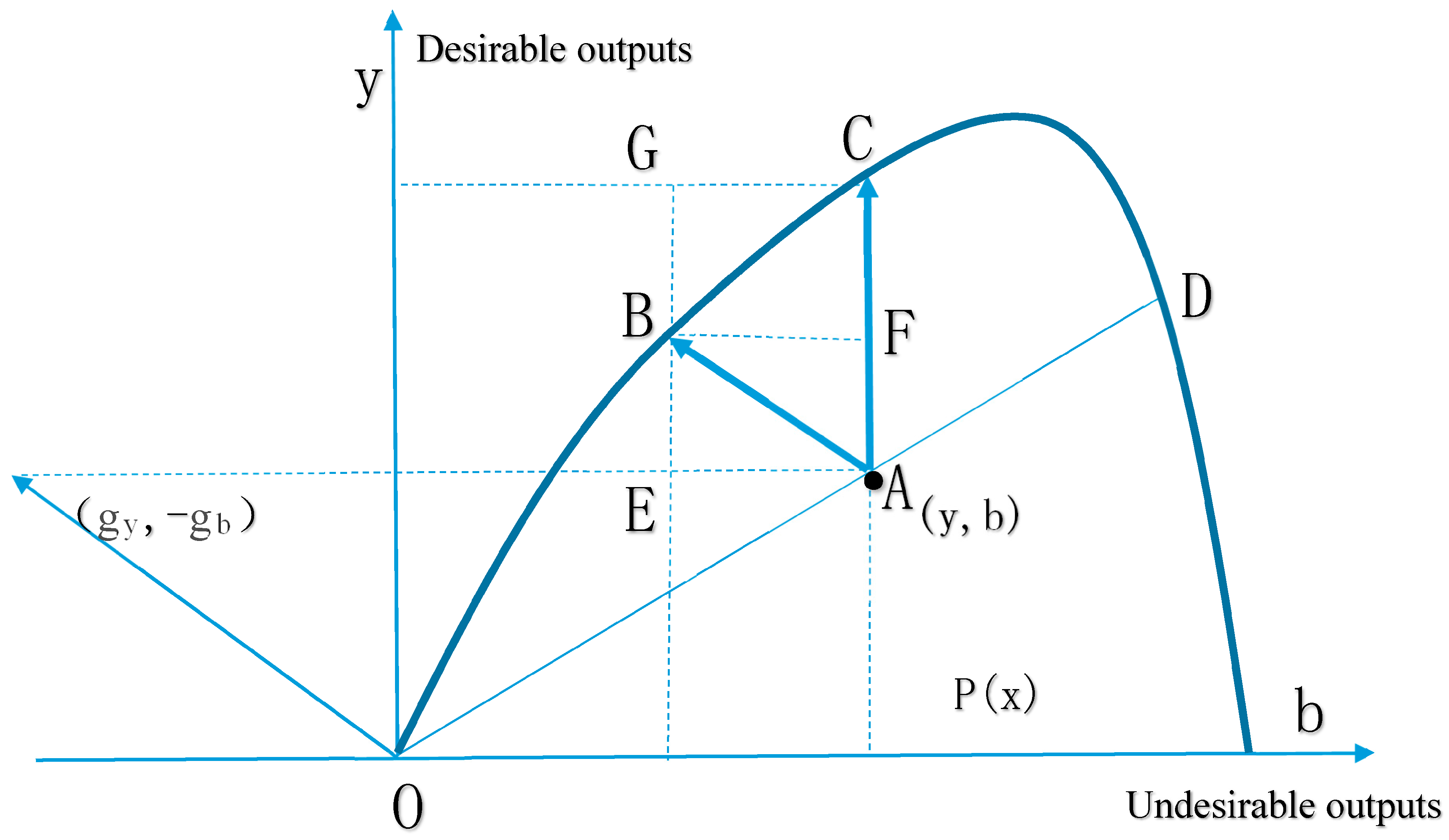
2.1. Directional Output Distance Function

The shadow prices of undesirable outputs can be derived by using a radial output/input distance function or a directional (output) distance function [12]. In this study, we adopt the directional distance function (DDF) method, which allows us to model the production of both good and bad outputs and provides a practical and flexible approach for assessing the shadow prices of carbon emissions.

First, the DDF is introduced as the representation of the production model. Assume that a production process involves N inputs denoted by $x=\left(x_1,\dots ,x_N\right)\in R_{+}^N$, M desirable outputs denoted by $y=\left(y_1,\dots ,y_M\right)\in R_{+}^M$ and J undesirable outputs denoted by $b=\left(b_1,\dots ,b_J\right)\in R_{+}^J$. The production technology can be described as

$$P\left(x\right)=\left\{\left(y,b\right):x can produce\left(y,b\right)\right\}$$

(1)

According to Färe et al. [28], some standard assumptions are imposed on the output sets $P\left(x\right)$: inputs are compact and freely disposable. Also, three nonstandard assumptions are imposed on them [18,28]. First, desirable and undesirable outputs are weakly disposable. Second, the desirable outputs by themselves are freely disposable. Third, the undesirable outputs are jointly produced with desirable outputs. Following the above assumptions, the directional output distance function that represents the production technology can be defined as

$${\overrightarrow{D}}_o\left(x,y,b;g_y,g_b\right)=max\left\{\beta :\left(y+\beta g_y,b-\beta g_b\right)\in P\left(x\right)\right\}.$$

(2)

$g=\left(g_y,g_b\right)>0$ denotes a directional vector. $\left(y+\beta g_y,b-\beta g_b\right)$ means that desirable outputs expand $\beta g_y$ and undesirable outputs simultaneously contract $\beta g_b$ where $\beta$ is the coefficient of expansion and contraction. Thus, the directional output distance Function (2) represents the maximum feasible changes of both desirable and undesirable outputs when they hit the boundary of the given production technology, $P\left(x\right)$.

According to Färe et al. [10], thanks to the assumptions previously imposed, the directional output distance function, ${\overrightarrow{D}}_o$, inherits its properties from the production technology, $P\left(x\right)$, including that ${\overrightarrow{D}}_o$ is monotonic, concave and non-negative for feasible output vectors; ${\overrightarrow{D}}_o$ is freely disposable in inputs and in desirable outputs; ${\overrightarrow{D}}_o$ is weakly disposable in undesirable outputs; ${\overrightarrow{D}}_o$ has a translational property.

$${\overrightarrow{D}}_o\left(x,y+\alpha g_y,b-\alpha g_b;g\right)={\overrightarrow{D}}_o\left(x,y,b;g\right)-\alpha$$

(3)

2.2. Shadow Prices of Undesirable Output

To derive the shadow prices of undesirable outputs, the relationship between the directional output distance function and the revenue function has to be clarified [7]. The revenue function is defined as

$$R\left(x,p,q\right)=\underset{y,b}{\max }\left\{py-qb:\left(y,b\right)\in P\left(x\right)\right\}$$

(4)

where $p=\left(p_1,\dots ,p_M\right)\in R_{+}^M$ denotes the desirable outputs’ prices and $q=\left(q_1,\dots ,q_J\right)\in R_{+}^J$ denotes the undesirable outputs’ prices.

The revenue function describes the maximum feasible output value, with both desirable and undesirable outputs taken into consideration. As the translation property (Equation (3)) implies, the producer moving from the feasible output vector $\left(y,b\right)$ along the direction $\left(g_y,-g_b\right)$ will cause an increase in desirable outputs and a decrease in undesirable outputs, which means a shrinkage of inefficiency. Thus, given the feasible directional vector, $g=\left(g_y,g_b\right)$, we can write

$$R\left(x,p,q\right)\ge \left(py-qb\right)+p·{\overrightarrow{D}}_o\left(x,y,b;g\right)·g_y+q·{\overrightarrow{D}}_o\left(x,y,b;g\right)·g_b$$

(5)

where $(p·{\overrightarrow{D}}_o\left(x,y,b;g\right)·g_y)$ and $(q·{\overrightarrow{D}}_o\left(x,y,b;g\right)·g_b)$ represent revenue increases resulting from desirable output increases and undesirable output decreases, respectively. Equation (5) becomes an equality when the producer reaches the frontier of $P\left(x\right)$ and the production is therefore efficient. Also, we can write Equation (5) as

$${\overrightarrow{D}}_o\left(x,y,b;g\right)\le \frac{R\left(x,p,q\right)-\left(py-qb\right)}{p{g}_y+q{g}_b}$$

(6)

Moreover, if it holds with equality, we have

$${\overrightarrow{D}}_o\left(x,y,b;g\right)=mi{n}_{p,q}\left\{\frac{R\left(x,p,q\right)-\left(py-qb\right)}{p{g}_y+q{g}_b}\right\}$$

(7)

Applying the envelope theorem to (Equation 7) we have

$${\nabla }_y{\overrightarrow{D}}_o\left(x,y,b;g\right)=\frac{-p}{p{g}_y+q{g}_b}\le 0$$

(8)

and

$${\nabla }_b{\overrightarrow{D}}_o\left(x,y,b;g\right)=\frac{q}{p{g}_y+q{g}_b}\ge 0$$

(9)

Given the market price of the mth desirable output is p_m, the shadow price of the jth undesirable output is

$$q_j=-p_m·\left(\frac{\partial {\overrightarrow{D}}_o\left(x,y,b;g\right)}{\partial b_j}/\frac{\partial {\overrightarrow{D}}_o\left(x,y,b;g\right)}{\partial y_m}\right)$$

(10)

Equation (10) informs us that the shadow price is determined by the marginal transformation rate between the desirable and undesirable outputs on the production frontier.

To put this differently, we illustrate this process in Figure 1. Given an output vector, A(y, b), located in $P\left(x\right)$ that represents the production technology, and a directional vector, $g=\left(g_y,g_b\right)>0$, point A can be mapped to point B along the direction, $\left(g_y,-g_b\right)$, resulting in an increase in desirable outputs and a decrease in undesirable outputs for a given input. The value of the DDF represents the maximum proportional change of the desirable and undesirable outputs. Assuming that the value of DDF is α₁, the desirable outputs expand (α₁g_y) and the undesirable outputs contract (α₁g_b). In contrast, the traditional Shephard distance function is a special case of the directional output distance function where the directional vector, $g^{″}=\left(y,-b\right)$, follows a direction that leads A to D, expanding both the desirable and undesirable outputs simultaneously.

Boyd et al. [29] have defined an alternative DDF to assess the marginal costs of undesirable outputs. Given another directional vector, $g^{\prime }=\left(g_y^{\prime },0\right)$, that directs point A to point C on the frontier, the maximum proportional increase of desirable outputs (α₂) is obtained while the inputs and undesirable outputs remain unchanged. By comparing DDF with alternative DDFs, thereby representing two kinds of environmental constrained activities, we are able to estimate the marginal abatement costs of undesirable outputs. Let $\mathrm{EB}={\alpha }_1{g}_y$ and $\mathrm{EA}={\alpha }_1{g}_b$ represent DDF; $\mathrm{EG}=\mathrm{AC}={\alpha }_2{g}_y^{\prime }$ represents the alternative DDF. Then, $\mathrm{BG}=\mathrm{EG}-\mathrm{EB}={\alpha }_2{g}_y^{\prime }-{\alpha }_1{g}_y$ is the loss of desirable outputs resulting from the contraction of undesirable outputs (EA). Therefore, the marginal abatement costs of undesirable outputs is given by

$$\left(p·\mathrm{BG}\right)/\left(q·\mathrm{EA}\right)=p\left({\alpha }_2{g}_y^{\prime }-{\alpha }_1{g}_y\right)/\left(q{\alpha }_1{g}_b\right)$$

(11)

where p and q denote the desirable and undesirable outputs’ prices.

3. Data and Results

3.1. Data

In this section we provide the definitions of our data sets, including inputs, and desirable and undesirable outputs. We consider a case with seven inputs (land, labor, fertilizer, pesticide, plastic film, irrigation and energy), one desirable output (economic output) and one undesirable output (carbon emission). All our data are from China Rural Statistical Yearbooks and China Agricultural Statistical Yearbooks. The data are available for 30 provinces in mainland China over the period from 1997 to 2014 and constitute a province-by-year panel. Hong Kong, Macao, Taiwan, Tibet have been excluded from the sample due to missing data.

We employed the sown area as a proxy for land in order to eliminate the effect of multiple cropping. Labor was measured as the total rural work force at the end of each year. Fertilizer, pesticide, plastic film and irrigation are the necessary material inputs used to produce crops. Energy represented the consumption of fuels and electricity by mechanical work. The desirable output in this study was the gross output value of the planting industry at 2000 constant prices. Since China has not promulgated the provincial data for carbon emissions in the agricultural sector, in accordance with Wu et al. [30] and Tian et al. [31] the estimation was as follows:

$$c={{\displaystyle \sum }}^{\text{}}{c}_i={{\displaystyle \sum }}^{\text{}}{e}_i·{\epsilon }_i$$

(12)

where c is the total carbon emissions and c_i is the emissions from each source. e_i is the amount of each emission source and ε_i is the emission coefficient of each source. In China’s planting industry, there are three main sources responsible for carbon emissions: (1) GHGs caused by carbon-generating activities, such as the utilization of fertilizer, pesticide and plastic film, and the consumption of fossil fuels and electrical energy during production processes; (2) CH₄, a potent GHG, generated in paddy field during rice growing process; (3) CO and CO₂ caused by crop straw burning on the farmland. We refer the reader interested in the details and derivation of the emission coefficients to Wu et al. [30] and Tian et al. [31]. To facilitate our analysis, we boiled down the GHG emissions into carbon equivalents, in accordance with the IPCC Fourth Assessment Report (2007), such that the greenhouse effect caused by 1 t N₂O and 1 t CH₄ is equivalent to that caused by 298 t CO₂ (81.2727 t C) and 25 t CO₂ (6.8182 t C), respectively. Descriptive statistics for the outputs and inputs are provided in

Table 1. Descriptive statistics of inputs and outputs (30 provinces, 18 years, 1997–2014).

	Variable	Units	Mean	SD	Max	Min
Inputs	Land	103 hectares	5237.18	3453.16	14,378.3	196.1
	Labor	104 persons	1050.34	771.09	3564	37.09
	Fertilizer	104 tonnes	163.58	130.51	705.75	6.57
	Pesticide	tonnes	50,319.36	42,425.85	198,764	1345
	Plastic film	tonnes	59,923.7	57,696.79	343,524	113
	Irrigation	103 hectares	1891.99	1415.56	5342.1	143.1
	Energy	104 kilowatts	2426.85	2491.61	13,101.4	95.3
Desirable output	Gross output	108 Yuan	592.60	454.12	2433.78	23.52
Undesirable output	Carbon equivalent	104 tonnes	760.04	581.03	2187.45	17.77

.

3.2. The Empirical Results

With the methods and data above, we conducted statistical analyses using Max DEA 5.0 software.

Table 2. Descriptive statistics of the regional shadow prices.

Region a	Mean b	SD	Max	Min
Northern China	113.26	132.12	530.1	8.01
Northeastern China	15.07	6.18	30.62	5.15
Eastern China	28.57	44.87	183.6	5.44
Central China	6.96	2.06	12.32	4.36
Southern China	34.36	32.44	90.98	10.73
Southwestern China	27.65	11	48.73	10.28
Northwestern China	187.35	246.73	820.76	18.34
Nationwide	66.1	132.63	820.76	4.36

^a The geographical regionalization here includes all provinces, except for Hong Kong, Macao, Taiwan and Tibet. Northern China includes Beijing, Tianjin, Hebei, Shanxi and Inner Mongolia; Northeastern China includes Liaoning, Jilin and Heilongjiang; Eastern China includes Shanghai, Jiangsu, Zhejiang, Fujian, Anhui, Jiangxi and Shandong; Central China includes Henan, Hubei and Hunan; Southern China includes Guangdong, Guangxi and Hainan; Southwestern China includes Sichuan, Chongqing, Yunnan and Guizhou; Northwestern China includes Shaanxi, Gansu, Xinjiang and Ningxia. ^b The estimates displayed are the simple arithmetic averages for the observations.

presents the descriptive statistics of the shadow prices on a regional level. Of the 540 observations, 90 are from Northern China, 54 from Northeast China, 126 from Eastern China, 54 from Central China, 54 from Southern China, 72 from Southwestern China and 90 from Northwestern China. The minimum shadow price (4.36 Yuan/tonne) appeared in Central China, while the maximum in was in Northwest China (820.76 Yuan/tonne). Furthermore, these two regions had the smallest and largest mean values of shadow prices (6.96 and 187.35) as well as standard deviation values (2.06 and 246.76). The large standard deviations in the statistics indicate substantial diversity in shadow prices. The average shadow price countrywide was 66.1 Yuan/tonne, but interestingly, the mean values of shadow prices in Northern China and Northwestern China were significantly higher than those in other regions, which is not in line with the results of some previous studies on China’s other sectors. We will further discuss this case in Section 4.

It can be seen in

Table 3. Shadow prices of carbon emissions in the planting industry from 1997 to 2014.

Province	1997	2000	2003	2006	2009	2012	2014	Mean	Growth Rate
Beijing	105.07	152.54	306.37	253.97	434.41	459.84	530.10	305.12	9.99%
Tianjin	129.13	164.30	216.71	172.09	183.30	205.07	260.94	184.01	4.22%
Hebei	12.15	12.29	11.36	8.56	9.02	8.54	8.23	9.83	−2.27%
Shanxi	44.71	52.51	49.10	25.58	24.89	19.58	18.87	33.38	−4.95%
Inner Mongolia	37.27	37.70	37.53	28.14	36.38	35.18	27.85	33.97	−1.70%
Liaoning	28.66	30.62	24.16	18.70	18.89	14.83	16.58	20.83	−3.17%
Jilin	20.83	22.11	13.60	10.34	12.60	8.92	8.52	13.61	−5.12%
Heilongjiang	17.55	16.07	14.48	9.55	7.12	5.61	5.15	10.78	−6.96%
Shanghai	78.84	80.82	137.85	133.54	165.24	176.45	183.60	130.88	5.10%
Jiangsu	6.33	6.74	7.96	6.77	7.61	7.38	7.27	7.10	0.82%
Zhejiang	12.50	13.51	16.74	15.83	15.96	16.48	15.68	14.68	1.35%
Anhui	8.55	8.06	6.99	6.18	5.93	5.56	5.44	6.73	−2.62%
Fujian	25.12	25.56	25.87	25.46	26.18	25.87	25.92	25.56	0.18%
Jiangxi	8.82	8.50	8.08	6.72	6.49	6.17	6.13	7.23	−2.11%
Shandong	9.34	8.62	8.38	7.17	7.40	7.15	7.24	7.84	−1.49%
Henan	12.32	11.01	10.15	8.53	7.92	7.34	7.26	9.23	−3.06%
Hubei	7.22	7.82	7.53	6.30	5.89	5.69	5.57	6.60	−1.52%
Hunan	6.05	5.57	5.66	4.99	4.55	4.37	4.36	5.06	−1.91%
Guangdong	10.73	11.48	13.02	13.04	12.65	12.23	12.19	12.30	0.76%
Guangxi	12.93	12.40	11.26	10.97	11.58	11.24	10.88	11.57	−1.01%
Hainan	88.50	88.63	85.93	79.68	69.47	68.14	66.50	79.20	−1.67%
Chongqing	34.80	31.73	29.60	28.36	28.49	29.20	28.64	29.99	−1.14%
Sichuan	13.24	12.04	11.87	10.91	10.54	10.41	10.33	11.28	−1.45%
Guizhou	48.73	45.64	36.22	34.06	32.63	32.70	33.22	37.80	−2.23%
Yunnan	42.59	38.53	32.10	27.80	28.86	24.67	22.90	31.52	−3.58%
Shaanxi	45.35	41.50	41.27	37.92	33.58	28.54	28.59	37.36	−2.68%
Gansu	68.98	68.89	63.22	59.40	44.01	38.36	35.46	53.56	−3.84%
Qinghai	667.12	647.75	760.97	711.81	645.62	560.03	527.15	664.35	−1.38%
Ningxia	209.09	183.27	183.59	154.93	124.20	108.74	106.01	149.80	−3.92%
Xinjiang	39.31	39.59	40.15	33.46	25.90	21.49	18.34	31.69	−4.38%

that the diversity of the shadow prices on a provincial level was even more substantial, with the provincial mean values ranging from 5.06 to 664.35 Yuan/tonne. The most notable was Qinghai province, where the mean value was rated the highest (with 664.35 Yuan/tonne) among the observed areas, followed by Beijing with 305.12 Yuan/tonne, Tianjin with 184.01 Yuan/tonne and Shanghai with 130.88 Yuan/tonne. Hunan province is at the bottom of the list, with an estimate of 5.06 Yuan/tonne.

Also, the dynamic trends of shadow prices show great disparity. While most of them were characterized by a decreasing trend during the observed period, only a small number of them are on the rise. The prevalent drop in marginal abatement costs signifies the capacity for abatement increases during the observed period.

The provinces with increasing shadow prices were Beijing, Tianjin, Shanghai, Jiangsu, Zhejiang, Fujian and Guangdong, whose average annual growth rates were 9.9%, 4.22%, 5.10%, 0.82%, 1.35%, 0.18% and 0.76%, respectively, indicating that it is becoming more difficult to mitigate carbon emissions over time. Notably, they are all Eastern coastal areas, with the most developed economies and agricultural technologies in China.

The shadow prices of the remaining 23 provinces showed more or less downward trends, suggesting a prevalent drop in marginal abatement costs in China. The figures for grain-producing areas like Heilongjiang, Jilin, Shanxi, Liaoning and Henan provinces fell sharply, with average annual reduction rates of 6.96%, 5.12%, 4.95%, 3.17% and 3.06%, respectively; also, in pastoral and agricultural–pastoral areas like Xinjiang, Ningxia and Gansu, the shadow prices slumped by 4.38%, 3.92% and 3.84%, annually.

4. Discussion and Policy Implications

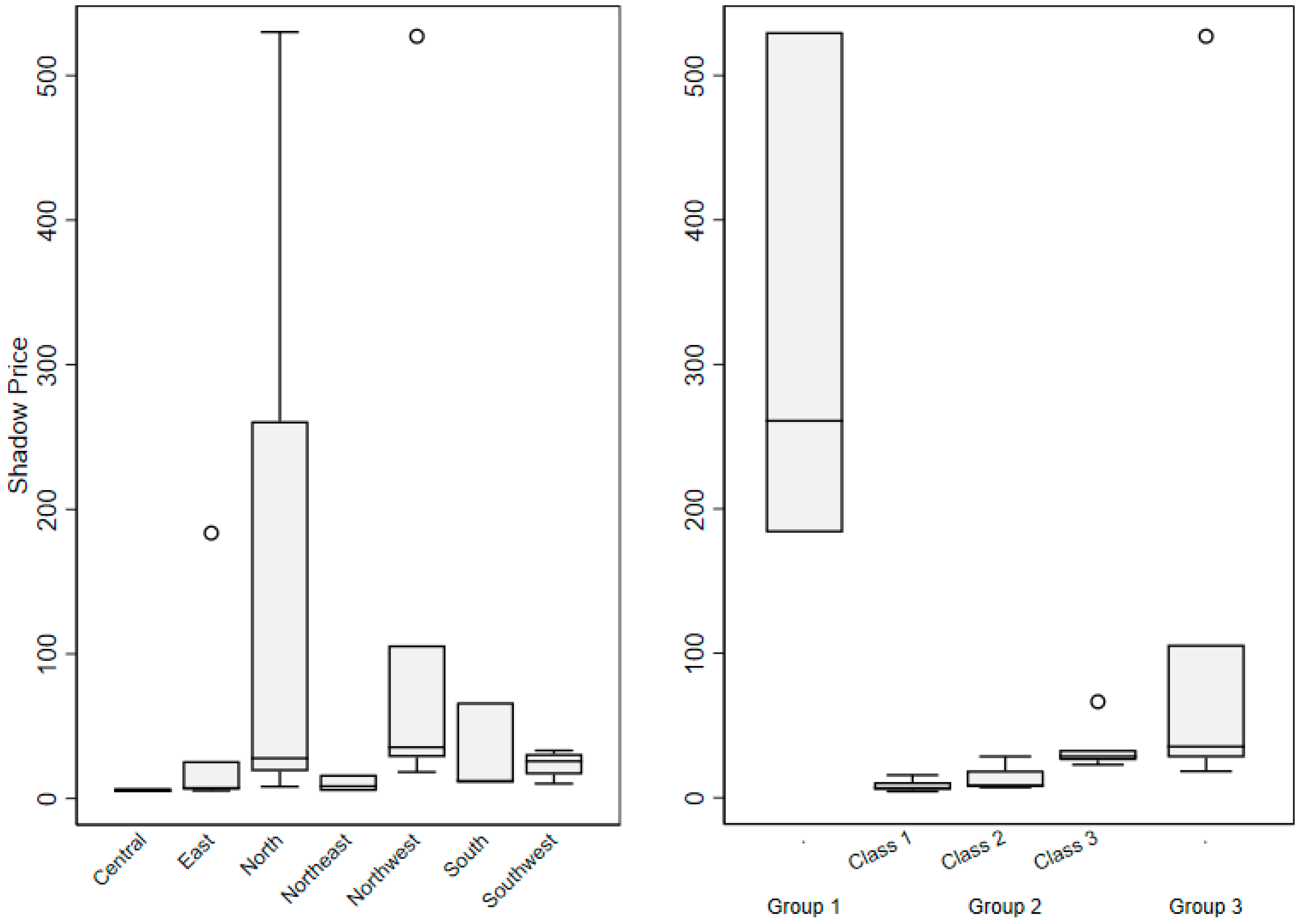
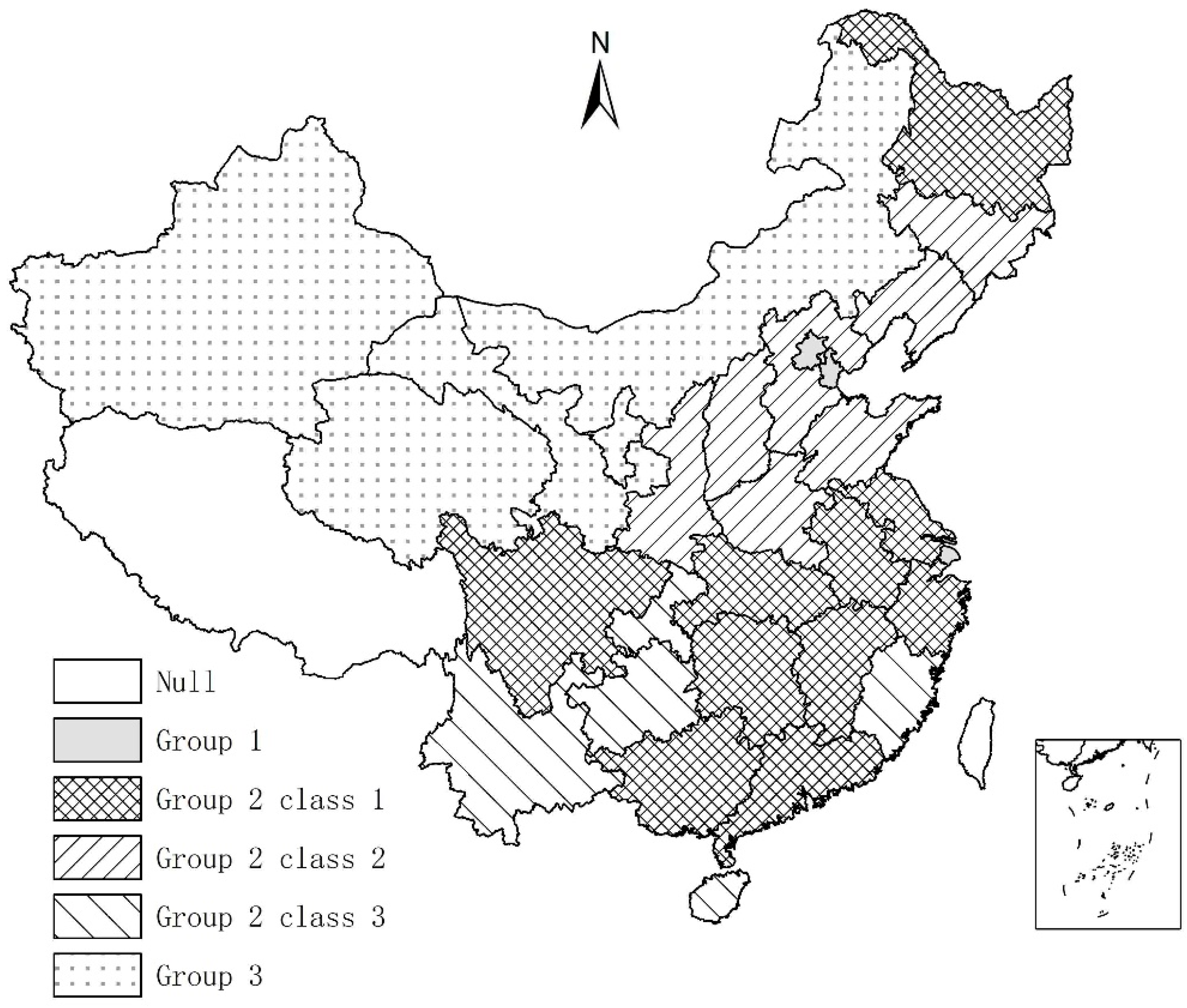
4.1. Regional Heterogeneity in the Shadow Prices

As is shown in Figure 2, there was considerable regional heterogeneity in the shadow prices. For our analysis, we divided the provinces into three groups according to their shadow price values. The first group consisted of Beijing, Tianjin and Shanghai—their shadow prices are at the top of the list. They share some common characteristics. For example, they are the most developed coastal areas with leading agricultural technologies, high value-added agricultural industries like leisure agriculture, and better industry convergence. They have higher levels of economic outputs and lower levels of carbon emissions. Specifically, the shadow prices in 2014 were 530.1 Yuan/tonne in Beijing, 260.94 Yuan/tonne in Tianjin and 183.6 Yuan/tonne in Shanghai, respectively. Higher shadow prices imply higher economic costs if these areas were to mitigate carbon emissions.

The second group, which had the lowest shadow prices, mainly includes provinces with planting industry predominating in their agriculture. Furthermore, we classified these provinces in terms of their shadow prices, regions and planting categories, as is shown in Figure 3. The excluded areas were of null value. Class 1 includes primary rice production regions, such as Hunan, Hubei, Jiangxi, Anhui, Sichuan, Jiangsu, Guangdong, Heilongjiang, etc. Class 2 includes areas mainly producing wheat, corn and Cereals, such as Henan, Hebei, Shandong, Shaanxi, Jilin, Liaoning, etc. Class 3 includes cash crop major producing provinces, like Hainan, Guizhou, Yunnan and Fujian. By and large, the later classes outnumber the former ones in terms of shadow prices. For example, class 1 provinces, primarily producing rice, like Hunan, Hubei, Anhui, Jiangsu and Jiangxi, have the lowest shadow prices nationwide—their mean shadow price is about 5–7 Yuan/tonne; class 3 provinces, such as Hainan (79.2 Yuan/tonne) and Guizhou (37.8 Yuan/tonne), have the highest shadow prices in this group. On the whole, the second group of provinces have vast areas of cultivated land and optimal climatic conditions for multiple cropping. A higher intensity of material input is needed to keep soil fertile and maintain productivity, giving rise to higher level of carbon emissions. The crop products, however, are generally priced at a relatively low level, resulting in the shadow prices being rated lowest among the observed provinces.

The third group of provinces had a medium level of shadow prices. They are mostly pastoral areas and agricultural–pastoral areas in Northern and Northwestern China, including Xinjiang, Gansu, Ningxia, Qinghai and Inner Mongolia. There are vast good grasslands for livestock to graze on, but crops there grow for less than two seasons per year due to the relatively cold and dry climatic conditions, which requires a lower intensity of material inputs. Moreover, compared to cereal crops, these areas are rich in higher value crop products, like cotton, oil plants, fruit crops and sugar crops. In this context, this group of provinces has higher shadow prices than the second group.

It is meaningful to compare the shadow prices in this paper with those of some other previous studies on other sectors. Broadly, the sequence of regional shadow prices in China, from high to low, is Eastern, middle and Western regions, in accordance with regional economic development levels (e.g., [19,20,22]). However, we reveal that the planting industry’s geographical distribution of shadow prices is quite different—the Northwestern provinces outnumber most middle and Eastern provinces in shadow prices, and Qinghai province has the highest shadow prices nationwide. The reason may well be that the planting industry is mostly labor intensive in China and is subject to natural resource and environmental constraints. The production efficiency in the less developed Northwestern regions is comparatively low owing to their lack of capital and labor resources, not enabling them to enjoy a full scale economy. However, many of them have a rich endowment of natural resources, and are in the increasing stage of scale returns, which means the enlargement of unit inputs could yield more outputs than some of the Eastern or middle regions, where the agricultural resources are, to some extent, over-exploited due to production technology. In this context, it is more costly to reduce an additional unit of carbon emission in such areas.

4.2. Policy Implications

China launched its much-awaited national carbon emission trading scheme (ETS) at the end of 2017, which is now the world’s largest carbon trading system [32,33]. However, this market primarily aims to limit China’s industrial sector’s emissions; its agricultural emissions still remain at large. China announced in the Paris Agreement to cut CO₂ emissions per unit of GDP by 60–65% by 2030, relative to 2005 levels [34]. To meet this challenging goal, it might be worth attempting to bring agriculture into line with China’s emission trading scheme. The regional heterogeneity in the marginal abatement costs strongly supports non-holding of the equimarginal principle and there is inefficiency of resource allocation among provinces. Theoretically, introducing an agricultural carbon market and taking shadow prices as the benchmark for trading under the frame of an emission cap may well be a solution that will help to motivate the reduction of inefficiency. Take China’s three Northeastern provinces, for example. The shadow prices of Liaoning, Jilin and Heilongjiang provinces in 2014 were 16.58, 8.52 and 5.15 Yuan/tonne, respectively. Assuming that their mean shadow price (10.08 Yuan/tonne) is set as the trading price, if, for example, every thousand tonnes of permits are traded, Jilin and Heilongjiang could acquire 1560 Yuan and 4930 Yuan in abatement compensation, while Liaoning could save 6500 Yuan. By means of such market adjustment, the permit-buyers would enlarge their production scales and their increased outputs would result in a decline in shadow prices. Conversely, the shadow prices of the sellers would rise. In the case of continuous trading, the shadow prices of both parties would eventually converge [23].

Agriculture in China, however, is a special sector, owing to the government’s goal of ensuring food security for its large population. China’s agricultural carbon trading should have its own framework, different from that of the industrial sectors. Compared with the results of some other studies (e.g., [22,23] in which the CO₂ shadow prices in China’s industrial sectors range from hundreds of Yuan to more than one hundred thousand Yuan and China’s national average shadow price is 1519 Yuan), the planting industry’s shadow prices are much lower. Hence, China should avoid making policy instruments that may motive a transfer of emission rights from agriculture to industry, which could be a great impediment to the development of agriculture. Also, it is thoughtless to simply drive the agricultural emissions from areas of low marginal abatement costs to areas where the costs are higher. On the basis of our results, shadow price is highly related to planting structure, implying that emission trading should be confined to the same crop categories or regions with similar crop structures, in order to keep an appropriate product mix and a quality structure of crops, in line with market needs. Therefore, a comprehensive, well-designed emission trading scheme is needed, not only to mitigate emissions, but also to maintain or adjust the crop structure and improve resource allocation efficiency.

Meanwhile, further efforts are required from governments to reverse the nationwide downward trend in shadow prices. They should take effective measures to enhance regional cooperation and learn from each other, especially from those with increasing shadow prices, in regard to carbon-reduction technology and experience. It is important to reduce their dependence on material production factors and improve the immaterial production factors’ contributions to the planting industry’s growth.

5. Conclusions

The shadow prices of carbon emissions play a vital role in assessing emission abatement costs and in supporting environmental policy making. In this paper we estimated the shadow prices of carbon emissions in China’s planting industry. We adopted a directional distance function that provided the most effective solution and allowed us to model the production of both economic output and carbon emissions. We used the best available data from 30 provinces from 1997 to 2014, and took into consideration the carbon emissions caused by three main emission sources from the planting industry. The shadow prices varied greatly among the provinces. Hunan, Hubei, Jiangsu and Jiangxi had the lowest shadow prices nationwide, while areas like Beijing, Tianjin and Shanghai had the highest shadow prices. Interestingly, the most undeveloped Northwestern provinces, like Xinjiang, Gansu, Ningxia, Qinghai and Inner Mongolia, unexpectedly outnumbered many Central and Eastern provinces in shadow prices. This is highly relevant to their regional planting structures. The analysis could provide some supporting information for policy recommendations, such as bringing agriculture into line with China’s current emission trading scheme, which could help to motivate the reduction of emissions and improve resource allocation among provinces. However, much work needs to be done for China’s inchoate emission trading market to live up to expectations.

In addition, the prevalent drop in shadow prices across the country shows that the capacity for abatement increased during the observed period. This implies further efforts are required from governments to reverse the nationwide downward trend in shadow prices. They should take effective measures to enhance regional cooperation and facilitate carbon-reduction technology transfer.

Finally, it should be noted that our study has its limitations. Our estimate does not include the carbon emissions that crops remove from the atmosphere by sequestering carbon in biomass and dead organic matter, because we lack reliable carbon sequestration coefficients for different crops from proven sources. The second limitation relates to the limited consideration of stochastic problems, because the assumption of weak disposability makes it difficult to employ random error models. How to introduce the stochastic analysis as well as carbon sinks as one of the desirable outputs to yield better estimates should be the next direction of research.

References

1. Dietz, T.; Gardner, G.T.; Gilligan, J.; Stern, P.C.; Vandenbergh, M.P. Household actions can provide a behavioral wedge to rapidly reduce US carbon emissions. Proc. Natl. Acad. Sci. USA 2009, 106, 18452–18456. [Google Scholar] [CrossRef] [PubMed]
2. Global Carbon Project: Global Carbon Atlas 2017. Available online: http://www.globalcarbonatlas.org/en/CO2-emissions (accessed on 25 November 2017).
3. Food Emissions. Available online: https://ccafs.cgiar.org/bigfacts/#theme=food-emissions&subtheme=direct-agriculture (accessed on 30 November 2017).
4. Tian, Y.; Zhang, J.B.; Li, B. Agricultural carbon emissions in China: Calculation, spatial-temporal comparison and decoupling effects. Resour. Sci. 2012, 34, 2097–2105. (In Chinese) [Google Scholar]
5. Hailu, A.; Veeman, T.S. Environmentally Sensitive Productivity Analysis of the Canadian Pulp and Paper Industry, 1959–1994: An Input Distance Function Approach. J. Environ. Econ. Manag. 2000, 40, 251–274. [Google Scholar] [CrossRef]
6. Lee, M. The shadow price of substitutable sulfur in the US electric power plant: A distance function approach. J. Environ. Manag. 2005, 77, 104–110. [Google Scholar] [CrossRef] [PubMed]
7. Fare, R.; Grosskopf, S.; Lovell, C.; Yaisawarng, S. Derivation of Shadow Prices for Undesirable Outputs: A Distance Function Approach. Rev. Econ. Stat. 1993, 75, 374–380. [Google Scholar] [CrossRef]
8. Lee, J.D.; Park, J.B.; Kim, T.Y. Estimation of the shadow prices of pollutants with production/environment inefficiency taken into account: A nonparametric directional distance function approach. J. Environ. Manag. 2002, 64, 365–375. [Google Scholar] [CrossRef]
9. Atkinson, S.E.; Dorfman, J.H. Bayesian measurement of productivity and efficiency in the presence of undesirable outputs: Crediting electric utilities for reducing air pollution. J. Econom. 2005, 126, 445–468. [Google Scholar] [CrossRef]
10. Färe, R.; Grosskopf, S.; Noh, D.W.; Weber, W. Characteristics of a polluting technology: Theory and practice. J. Econom. 2005, 126, 469–492. [Google Scholar] [CrossRef]
11. Mekaroonreung, M.; Johnson, A.L. Estimating the shadow prices of SO2 and NOx for U.S. coal power plants: A convex nonparametric least squares approach. Energy Econ. 2012, 34, 723–732. [Google Scholar] [CrossRef]
12. Zhou, P.; Zhou, X.; Fan, L.W. On estimating shadow prices of undesirable outputs with efficiency models: A literature review. Appl. Energy 2014, 130, 799–806. [Google Scholar] [CrossRef]
13. Coggins, J.S.; Swinton, J.R. The Price of Pollution: A Dual Approach to Valuing SO2Allowances. J. Environ. Econ. Manag. 1996, 30, 58–72. [Google Scholar] [CrossRef]
14. Murty, M.N.; Kumar, S. Measuring the cost of environmentally sustainable industrial development in India: A distance function approach. Environ. Dev. Econ. 2002, 7, 467–486. [Google Scholar] [CrossRef]
15. Murty, M.N.; Kumar, S.; Paul, M. Environmental regulation, productive efficiency and cost of pollution abatement: A case study of the sugar industry in India. J. Environ. Manag. 2006, 79, 1–9. [Google Scholar] [CrossRef] [PubMed]
16. Hernández-Sancho, F.; Molinos-Senante, M.; Sala-Garrido, R. Economic valuation of environmental benefits from wastewater treatment processes: An empirical approach for Spain. Sci. Total Environ. 2010, 408, 953–957. [Google Scholar] [CrossRef] [PubMed]
17. Molinos-Senante, M.; Hanley, N.; Sala-Garrido, R. Measuring the CO2 shadow price for wastewater treatment: A directional distance function approach. Appl. Energy 2015, 144, 241–249. [Google Scholar] [CrossRef]
18. Molinos-Senante, M.; Guzmán, C. Reducing CO2 emissions from drinking water treatment plants: A shadow price approach. Appl. Energy 2016, 210, 623–631. [Google Scholar] [CrossRef]
19. Wei, C.; Ni, J.; Du, L. Regional allocation of carbon dioxide abatement in China. China Econ. Rev. 2012, 23, 552–565. [Google Scholar] [CrossRef]
20. Choi, Y.; Zhang, N.; Zhou, P. Efficiency and abatement costs of energy-related CO2 emissions in China: A slacks-based efficiency measure. Appl. Energy 2012, 98, 198–208. [Google Scholar] [CrossRef]
21. He, X.P. Regional differences in China’s CO2 abatement cost. Energy Policy 2015, 80, 145–152. [Google Scholar] [CrossRef]
22. Chen, D.H.; Pan, Y.C.; Wu, C.Y. Marginal abatement costs of CO2 emission in China and its regional differences. China Popul. Resour. Environ. 2016, 26, 86–93. (In Chinese) [Google Scholar]
23. Chen, S.Y. Shadow Price of CO2 from Industrial Sector: Parametric and Nonparametric Approaches. J. World Econ. 2010, 33, 93–111. (In Chinese) [Google Scholar]
24. Lee, M.; Zhang, N. Technical efficiency, shadow price of carbon dioxide emissions, and substitutability for energy in the Chinese manufacturing industries. Energy Econ. 2012, 34, 1492–1497. [Google Scholar] [CrossRef]
25. Chen, S.Y. What is the potential impact of a taxation system reform on carbon abatement and industrial growth in China? Econ. Syst. 2013, 37, 369–386. [Google Scholar] [CrossRef]
26. Wang, K.; Che, L.; Ma, C.; Wei, Y.M. The shadow price of CO2 emissions in China’s iron and steel industry. Sci. Total Environ. 2017, 598, 272–281. [Google Scholar] [CrossRef] [PubMed]
27. Wu, X.R.; Zhang, J.B.; Tian, Y.; Xue, L.F. Analysis on China’s Agricultural Carbon Abatement Capacity from the Perspective of Both Equity and Efficiency. J. Nat. Resour. 2015, 30, 1172–1182. (In Chinese) [Google Scholar]
28. Färe, R.; Grosskopf, S.; Weber, W.L. Shadow prices and pollution costs in U.S. agriculture. Ecol. Econ. 2006, 56, 89–103. [Google Scholar] [CrossRef]
29. Boyd, G.A.; Tolley, G.; Pang, J. Plant Level Productivity, Efficiency, and Environmental Performance of the Container Glass Industry. Environ. Resour. Econ. 2002, 23, 29–43. [Google Scholar] [CrossRef]
30. Wu, X.R.; Zhang, J.B.; Tian, Y.; Li, P. Provincial Agricultural Carbon Emissions in China: Calculation, Performance Change and Influencing Factors. Resour. Sci. 2014, 36, 129–138. (In Chinese) [Google Scholar]
31. Tian, Y.; Zhang, J.B.; He, Y.Y. Research on Spatial-Temporal Characteristics and Driving Factor of Agricultural Carbon Emissions in China. J. Integr. Agric. 2014, 13, 1393–1403. [Google Scholar] [CrossRef]
32. Energy Foundation: China Launches World’s Largest Carbon Trading System. Available online: https://www.ef.org/china-launches-worlds-largest-carbon-trading-system (accessed on 23 December 2017).
33. Chinanews: China Launches National Carbon Trading Scheme. Available online: http://www.ecns.cn/video/2017/12-20/285217.shtml (accessed on 20 December 2017).
34. Alfaenergy: US and China Ratiry Paris Climate Agreement. Available online: https://blog.alfaenergygroup.com/us-and-china-ratify-paris-climate-agreement/ (accessed on 13 September 2016).
Figure 1. The directional output distance function.
Sustainability 10 00753 g001
Figure 2. Distribution of shadow price values by region and group in 2014.
Sustainability 10 00753 g002
Figure 3. Geographical locations of groups of provinces.
Sustainability 10 00753 g003