Mapping Spring Ephemeral Plants in Northern Xinjiang, China

Abstract

Spring ephemeral plants (SEP) are a particular component of flora that take full advantage of water resources and temperature conditions to rapidly complete their life cycle in about two months. In China, they are mainly distributed in northern Xinjiang. They play important roles in dune stability and are precious food for the livestock and wild animals in the early spring. Northern Xinjiang is under dramatic climate changes and land-use/land-cover changes, which can affect the growth of SEP in this region. To explore how the distribution of SEP have varied under these changes, Moderate-Resolution Imaging Spectrodiometer (MODIS) Enhanced Vegetation Index (EVI) time series of two years (2000 and 2014) were applied to detect SEP in each period. The TIMESAT software was used to extract the seasonality information from the EVI data. The results show that SEP in northern Xinjiang are mainly located in the south of the Gurbantunggut desert and along the Ili Valley and piedmont hills of the mountains. In 2000, its total area was 3.83 × 10⁴ km², accounting for 10% of the entire region. By 2014, the total area was about 2.74 × 10⁴ km², with a decrease of 28.5% relative to 2000. Land-use/land-cover datasets can be used to determine whether changes in SEP over time are caused by human activities or natural factors. Combing the SEP maps with the synchronous land-use/land-cover datasets indicates that the decrease is mainly caused by natural factors, which are possibly related with the temperature and precipitation changes in this region. Human activities only contributed 4% to the decrease, with most SEP areas being replaced by croplands. The observed SEP dynamics and changes pertain only to the years with below-average precipitation.

1. Introduction

Spring ephemeral plants (SEP), also known as desert ephemerals, are a particular component of flora that take full advantage of water resources and temperature conditions to rapidly complete their life cycle in about two months. In China, they are mainly distributed in northern Xinjiang [1]. The ephemerals in this region play important roles in dune stabilization from April to June when the aeolian activity in the desert is strong and the coverage of trees, shrubs and herbs of long vegetative period is small [2]. They serve as a precious food for the livestock and wild animals in the early spring and also influence the region’s fire regime.

Numerous studies have shown that the natural vegetation in northern Xinjiang is sensitive to precipitation variation [3,4]. Moreover, SEP have stronger sensitivity to changes than non-SEP [5]. A minor percentage increase or decrease in the amount of precipitation can tip the balance between the ecosystem and climate and prompt for different flora in the region.

In northern Xinjiang, the annual precipitation has increased in the past century [6]. Meanwhile, its average surface air temperature has increased at a rate much larger than the global averaged [7,8]. Potential impacts of these changes on SEP should be examined and understood. Such understanding has become ever urgent in the face of rapid urbanization and reclamation in this region in the last decades [9]. Human activities can fragment the SEP habitats into patches and even eliminate them.

To explore how the distribution of SEP have varied under climate changes and human activities, Moderate-Resolution Imaging Spectrodiometer (MODIS) Enhanced Vegetation Index (EVI) time-series of two years (2000 and 2014) are applied to detect SEP in northern Xinjiang in each period. The SEP distribution in 2008 is also detected as a supplement to the analyses and discussion. The rule to classify SEP and non-SEP is based on the seasonality information (phenology parameters) extracted from the TIMESAT software.

2. Materials and Methods

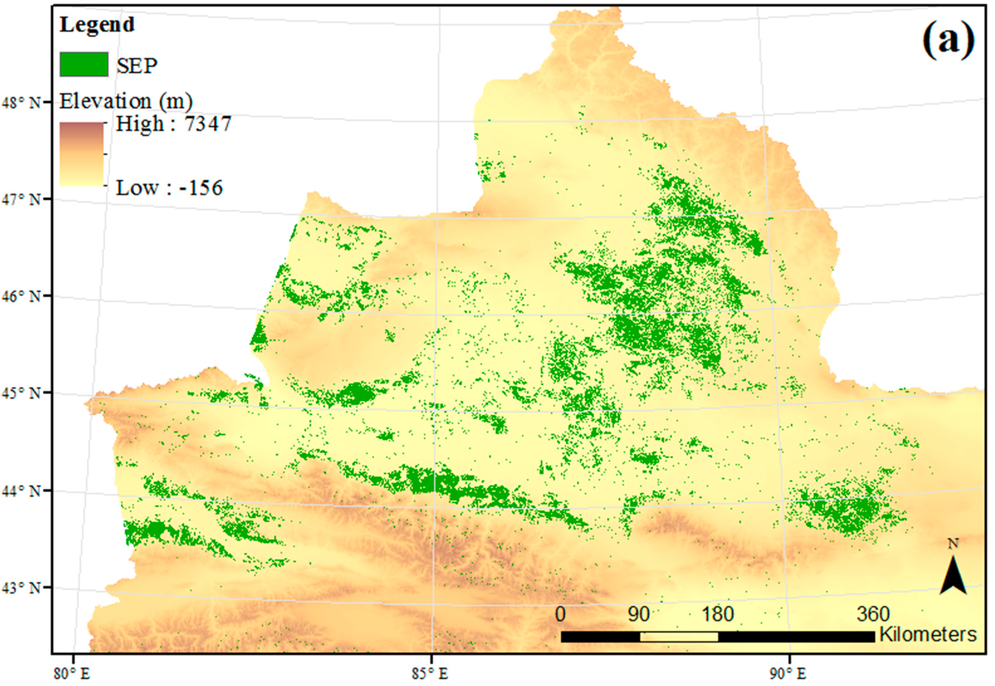
2.1. Study Area

The study area, in the north of Xinjiang province of China, consists of the Ili valley and the Junggar Basin (Figure 1). The whole area covers approximately 3.8 × 10⁵ km², ranging from 42° to 48° latitude and from 80° to 92° longitude. Geographically enclosed by the Tianshan Mountains, the Ili valley crosses the temperature continental and alpine climate, with average annual precipitation ranging from 200 to 800 mm and average annual temperature from 2.9 to 9.1 °C [10]. Vegetation in the valley is affected by the altitude and the mountain microclimate. The Junggar Basin is bounded by the Tianshan Mountains to the south and the Altay Mountains to the north. The Gurbantunggut Desert, China’s second largest, is in the center of the basin. The Junggar Basin is much drier than the Ili valley, with annual precipitation less than 100 mm over most of the area. Its temperature can fall below −20 °C in the winter and rise above 35 °C in the summer. The ephemerals grown in these two subregions generally sprout at the end of March/early April and wither by early June, with a life cycle of about two months. They are named spring ephemeral plants.

2.2. MODIS-EVI Data

MODIS is one of the key instruments aboard the Sun-synchronous Terra and Aqua Satellites. In this study, we used the vegetation index product MOD13Q1 Version 6 [11]. The 16-day product contains 12 layers at 250-m spatial resolution, of which the EVI and pixel reliability layers are applied. The EVI was developed to optimize the vegetation signal with improved sensitivity in high biomass regions and improved vegetation monitoring through a de-coupling of the canopy background signal and a reduction in atmosphere influences. The equation takes the form,

$$EVI=G\frac{{\rho }_{NIR}-{\rho }_{RED}}{{\rho }_{NIR}+C_1\times {\rho }_{RED}-C_2\times {\rho }_{BLUE}+L}$$

where $\rho$ are atmospherically corrected or partially atmospherically-corrected (Rayleigh and ozone absorption) surface reflectance, L is the canopy background adjustment that address nonlinear, different near infrared (NIR) and red radiant transfer through a canopy, and C₁, C₂ are the coefficients of the aerosol resistance term, which uses the blue band to correct for aerosol influences in the red band. The coefficients adopted in the EVI algorithm are, L = 1, C₁ = 6, C₂ = 7.5, and G (gain factor) = 2.5 [12,13].

MODIS datasets are delivered in sinusoidal projection and a tiling system, where each tile covers an area of approximately 1,440,000 km². Northern Xinjiang is covered by the tiles h23v04 and h24v04. For this work, we used the EVI time series of two years (2000 and 2014) to map the distribution of SEP in each period. There are twenty-three composites per year. In addition, the EVI data of 2008 is added when calibrating the TIMESAT software in Section 3 and debating the variation in 2014 relative to 2000 in Section 4. Note that the EVI data in this paper is in the original unit of 10⁻⁴ and 16-bit integer format, to reduce the data volume.

2.3. Land-Use/Land-Cover Data

Land-use/land-cover changes have links to both human and nature interactions. China’s Land-use/cover Datasets (CLUDs) were updated regularly at 5-year intervals from the late 1980s to 2015, with standard procedures based on Landsat images [14]. Here, the datasets in 2000 and 2015 are used to indicate the variation in land-use/land-cover in northern Xinjiang. Note that the dataset of 2015 can represent that condition in 2014, because the changes between them would be insignificant.

2.4. Fieldwork

Vegetation was surveyed in plots scattered across northern Xinjiang and yearly from 2009 to 2015 (as red crosses in Figure 1). The ephemerals in this region are generally low and have small canopies. Therefore, species numbers and crown diameters were documented in 10 m × 10 m quadrats. At least 3 quadrats were set in each survey site and they are placed according to the local geography. For example, quadrats in the desert were classified as dune-foot, dune-slope and dune-crest, respectively.

After the surveys, the plants in each quadrat were classified into two groups, ephemeral and long-lived plants, based on the length of the lifespan of each species. Ephemeral plants germinate in early spring and can complete their life history before summer arrives, having a lifespan of about 2 months. Although long-lived plants also germinate in early spring, they have a lifespan of about 5 months. Both ephemerals and long-lived plants are a mix of annuals and perennials. About 70 sites were surveyed during 2009–2015. Most of them were visited several times. However, only the sites with a mean relative coverage of the ephemerals larger than 10% were adopted in this study (n = 50).

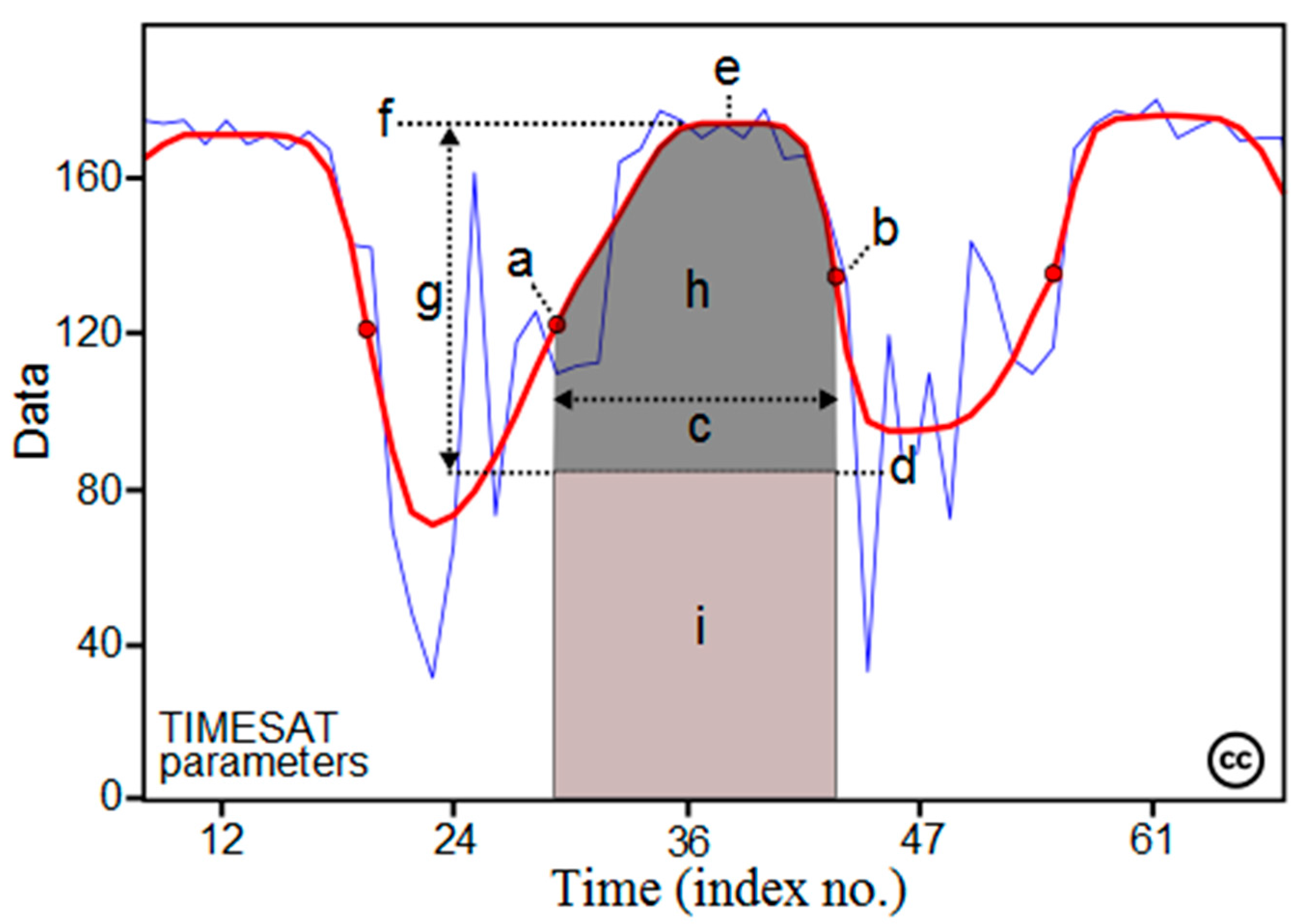
2.5. TIMESAT

The software TIMESAT 3.3 (Lars Eklundha and Per Jönssonb, Sweden) was used to handle noisy time series of EVI and extract seasonality information from the data for the study area [15,16,17]. It fits a smooth continuous curve to time series of EVI using Savitzky–Golay filtering (SG), asymmetrical Gaussian (AG), or double logistic (DL) functions, and an adaptive upper envelope to account for negatively biased noise such as cloud cover. Meanwhile, the pixel reliability labels accompanying the EVI data are used as ancillary quality data to detect the spikes and outliers, by assigning weights to the EVI values in the time-series. The pixel reliability data which lies between −1 and 3, represents no data (−1), good data (0), marginal data (1), snow/ice (2), and cloud cover (3). Values 0–3 are assigned a weight of 1, 1, 0.5 and 0.1, respectively. Assigning value 0 as a weight of 0.1 (instead of 0) is to reduce the risk of missing the season entirely caused by too many missing values with weight 0. Sensitivity tests (not shown) indicate that this setting has little effect on the extracted seasonality information.

Output from TIMESAT consists of 9 seasonality parameters (Figure 2), of which time of middle of season and amplitude are used in this study. Time of middle of season (hereafter called peak t.) indicates when the vegetation season peaks and amplitude is the difference between the base value and the maximum value in a single growing season. As discussed above, SEP dry up by early June. Therefore, their peak t. is before June. On the contrast, the peak t. of the long-lived vegetation (shrubs, forests and croplands) is much later. Based on the differences between SEP and non-SEP in the peak t., we can separate them apart. Meanwhile, amplitude is added to help the discrimination of SEP. It can remove the noises in the classification that are caused by minor fluctuation in the EVI signals.

3. Results

Calibration was required to select the smoothing technique, envelope size and other options in TIMESAT. In this work, 4 out of the 50 survey sites are chosen as training sites to calibrate the software with the EVI time series for the three years of 2000, 2008 and 2014. These four sites can represent different environmental conditions in northern Xinjiang (as summarized in

Table 1. Training sites for TIMESAT calibration.

Site Name	Latitude	Longitude	Environmental Condition	Main SEP Species
S1	44.23	85.21	Flat steppe	Ceratocephalus orthoceras DC.
S2	44.20	86.01	Piedmont hills	Ferula ferulaeoides (Steud.) Korov.
S3	44.46	88.16	Desert	Erodium oxyrrhynchum M.B.
S4	43.99	87.84	Piedmont hills	Tetracme quadricornis (Steph.) Bunge

). In addition, they were more frequently surveyed during 2009–2015 than the other sites. To overcome the problem that the TIMESAT software ignores the beginning and ending time-series of the EVI data in the procedure, we duplicate the data of 2000 and 2014. As a result, 5-year long data were analyzed for calibration and only the results in the middle three years were analyzed. Note that the first three time-series of the EVI data in 2000 are missed and a linear interpolation is used to fill the missing data before the smoothing process.

Here we focused on the calibration with three smoothing techniques (SG, AG, and DL). The fitted curves with these three smoothing techniques are shown in Figure 3 (X-axis refers to the Julian day of the composite). These results indicate that the fitted EVI curves with the SG function on all four training sites are closer to the raw curves than those with other smoothing techniques (AG and DL). It seems that the AG and DL functions are good at fitting smoother curves, not those of SEP with a very steep peak in each year. Therefore, the SG function was applied in this study. In addition, we set Seasonal par. as 1, No. of envelope iterations as 2, Adaption strength as 2, and Savitsky–Golay window size as 4.

Then, the TIMESAT software with optimized options were applied over northern Xinjiang with the EVI images during 2000, 2008 and 2014. The calculated seasonality parameters were also stored as images.

To detect SEP with peak t. and amplitude, the threshold values of these two parameters for SEP in the study area should be set. Take peak t. as an example. First, the peak t. values of the 50 survey sites in 2000, 2008 and 2014 are extracted from the output of TIMESAT. Figure 4a shows the frequency of the peak t. sample and its fitted normalized distribution. The mean of the normalized distribution is 32.01 and its standard deviation is 0.75. About 95% of the sample are within two standard deviation (μ ± 2σ). So we set the lower and upper threshold of the peak t. values for SEP as 30.51 (middle April) and 33.52 (late May), respectively. In the same way, the lower and upper threshold of the amplitude values for SEP are set as 438 and 3089, respectively (Figure 4b).

Based on the identified ranges of the peak t. (30.51–33.52) and amplitude (438–3089) for SEP, the distribution of SEP in 2000 and 2014 are mapped. Figure 5a shows the distribution of SEP in 2000. It was found that SEP spread over northern Xinjiang, from the Ili Valley to the east edge of the Gurbantunggut Desert and from the piedmont hills of the Altay Mountains to those of the Tianshan Mountains. The total area was approximately 3.83 × 10⁴ km², accounting for 10% of the entire region. Figure 5b shows the distribution of SEP in 2014. The total area was about 2.74 × 10⁴ km², accounting for 7% of the entire region. Figure 5a,b both indicate that SEP in northern Xinjiang are mainly located in south of the Gurbantunggut desert and along the Ili Valley and piedmont hills of the mountains.

To assess the accuracy of the classification method, we compared the resultant map in 2014 with the product of 2015 from CLUDs. It was found that the ephemerals in our map generally did not overlap with the non-ephemeral classes (farmland, forest, water bodies, and urban and built-up land) in the land-use/cover image. To quantitatively estimate the error of commission, 5000 samples belonging to the non-ephemeral classes were randomly selected from the land-use/cover image. By overlapping the non-SEP samples on our map, only 95 out of the samples were wrongly identified as the ephemerals, with the user’s accuracy as high as 98.1%.

The total area of SEP has decreased by 28.5% from 2000 to 2014. Figure 6b shows the details regarding the variation. It was found that transition from SEP to non-SEP mainly occurred in the northeastern part of the Junggar Basin, the southeastern edge of the basin and northern part of the Gurbantunggut desert. Moreover, it occurred in some small areas along the Ili Valley and the piedmont hills in the western part of the basin. Transition from non-SEP to SEP mainly occurred in the southern part of the Gurbantunggut desert and along the piedmont hills of the Tianshan Mountains ranging from 85 to 89 longitude. Of course, the area from SEP to non-SEP was larger than that from non-SEP to SEP, which resulted in a decrease in the total area of SEP from 2000 to 2014.

4. Discussion

As discussed above, precipitation is a key factor controlling vegetation growth in northern Xinjiang. Vegetation phenology and seasonality information can vary among the years with different dry/wet conditions. To reduce the inconsistency in the seasonality parameters between different years when studying the variation in the distribution of SEP, the EVI time series of three years (2000, 2008, and 2014) with similar precipitation amount in the spring (March–May) were applied. Moreover, the precipitation amount of these three years was below the average value (83 mm) of the past 30 years. The dry conditions can increase the difference between ephemeral and long-lived vegetation in the EVI signals, which favors the discrimination of SEP.

Considering that SEP species have short life cycles and a strong dependence on annual climatic conditions (especially timing and amount of precipitation), comparing two years (2000 and 2014) may not be enough to fully detect the habitat loss. As a result, variation in 2008 is also detected (Figure 6a). When comparing results of 2008 with those of 2014 (Figure 6a vs. 6b), it’s found the patterns are similar and the variation from 2000 to 2014 is continuous. For example, the ephemerals on the east edge of the Junggar Basin started to disappear in the south (Figure 6a) and then the shrinking extended to the north (Figure 6b). Similar changes are also found in the Ili Valley. This demonstrates that the variation in the distribution of SEP reported in this study is credible.

Land-use/cover Datasets can reveal whether the land-use/land-cover changes are caused by human activities or natural factors. By combing the datasets of 2000 and 2015 from CLUDs with the maps of SEP, we found that human activities only contributed 4% to the transition from SEP to non-SEP, with these SEP areas being replaced by croplands. The remaining 96% of the transition from SEP to non-SEP is contributed by natural factors, which are possibly related to the precipitation and temperature changes in this region. Further study is needed to explain how SEP responds to the changing climate.

In this work, the observed SEP dynamics and changes pertain only to the years with below-average precipitation, which may bring possible limitations and impact on the findings. More data, ideally the entire 2000–2018 time-series, are suggested for further study.

References

- Mao, Z.; Zhang, D. The conspectus of ephemeral flora in northern xinjiang. Arid Zone Res. 1994, 11, 1–26. [Google Scholar]
- Wang, X.; Jiang, J.; Lei, J.; Zhang, W.; Qian, Y. Distribution of ephemeral plants and their significance in dune stabilization in gurbantunggut desert. J. Geogr. Sci. 2013, 13, 323–330. [Google Scholar]
- Gessner, U.; Naeimi, V.; Klein, I.; Kuenzer, C.; Klein, D.; Dech, S. The relationship between precipitation anomalies and satellite-derived vegetation activity in central asia. Glob. Planet Chang. 2013, 110, 74–87. [Google Scholar] [CrossRef]
- Zhang, C.; Lu, D.; Chen, X.; Zhang, Y.; Maisupova, B.; Tao, Y. The spatiotemporal patterns of vegetation coverage and biomass of the temperate deserts in central asia and their relationships with climate controls. Remote Sens. Environ. 2016, 175, 271–281. [Google Scholar] [CrossRef]
- Wang, X.; Jiang, J.; Wang, Y.; Luo, W.; Song, C.; Chen, J. Responses of ephemeral plant germination and growth to water and heat conditions in the southern part of gurbantunggut desert. Chin. Sci. Bull. 2006, 51, 110–116. [Google Scholar] [CrossRef]
- Hu, Z.; Zhou, Q.; Chen, X.; Qian, C.; Wang, S.; Li, J. Variations and changes of annual precipitation in central asia over the last century. Int. J. Climatol. 2017, 37, 157–170. [Google Scholar] [CrossRef]
- Chen, F.; Wang, J.; Jin, L.; Zhang, Q.; Li, J.; Chen, J. Rapid warming in mid-latitude central asia for the past 100 years. Front. Earth Sci. Chin. 2009, 3, 42–50. [Google Scholar] [CrossRef]
- Hu, Z.; Zhang, C.; Hu, Q.; Tian, H. Temperature changes in central asia from 1979 to 2011 based on multiple datasets. J. Clim. 2014, 27, 1143–1167. [Google Scholar] [CrossRef]
- Wu, Y.; Wu, S.; Zhang, J.; Liu, M. Study of xinjiang oasis with multitude of temporal and spatial data. Arid Land Geogr. 2014, 37, 333–341. (In Chinese) [Google Scholar]
- Domrös, M.; Peng, G. The Climate of China; Springer Science & Business Media: Berlin, Germany, 2012. [Google Scholar]
- Huete, A.; Didan, K.; Miura, T.; Rodriguez, E.P.; Gao, X.; Ferreira, L.G. Overview of the radiometric and biophysical performance of the modis vegetation indices. Remote Sens. Environ. 2002, 83, 195–213. [Google Scholar] [CrossRef]
- Huete, A.R.; Liu, H.Q.; Batchily, K.; van Leeuwen, W. A comparison of vegetation indices global set of tm images for eos-modis. Remote Sens. Environ. 1997, 59, 440–451. [Google Scholar] [CrossRef]
- Huete, A.; Justice, C.; Liu, H. Development of vegetation and soil indexes for modis-eos. Remote Sens. Environ. 1994, 49, 224–234. [Google Scholar] [CrossRef]
- Liu, J.; Kuang, W.; Zhang, Z.; Xu, X.; Qin, Y.; Ning, J.; Zhou, W.; Zhang, S.; Li, R.; Yan, C. Spatiotemporal characteristics, patterns, and causes of land-use changes in china since the late 1980s. J. Geogr. Sci. 2014, 24, 195–210. [Google Scholar] [CrossRef]
- Jonsson, P.; Eklundh, L. Timesat—A program for analyzing time-series of satellite sensor data. Comput. Geosci. 2004, 30, 833–845. [Google Scholar] [CrossRef]
- Jonsson, P.; Eklundh, L. Timesat 3.3 with Seasonal Trend Decomposition and Parallel Processing Software Manual; Lund and Malmö University: Lund, Sweden, 2017. [Google Scholar]
- Jonsson, P.; Eklundh, L. Seasonality extraction and noise removal by function fitting to time-series of satellite sensor data. IEEE Trans. Geosci. Remote Sens. 2002, 40, 1824–1832. [Google Scholar] [CrossRef]