A Dynamic Analysis to Evaluate the Environmental Performance of Cities in China

1
School of Management, Harbin Institute of Technology, Harbin 150001, China
2
School of Management, Guangzhou University, Guangzhou 510006, China
*
Author to whom correspondence should be addressed.
Sustainability 2018, 10(3), 862; https://doi.org/10.3390/su10030862
Submission received: 10 January 2018
/
Revised: 15 March 2018
/
Accepted: 16 March 2018
/
Published: 19 March 2018
Abstract
:With the contradiction between energy supply and demand around the world, urbanization formed with high-investment, high-consumption, and high-emission has significantly impaired the ecological environment of China. The evaluation of environmental impact is a must for decision-makings related to sustainable urbanization. This paper assessed the dynamic environmental performance of 285 cities in China from 2005 to 2013 based on the Malmquist-Luenberger index, an expanded data envelopment analysis (DEA) model. To ensure comparability among cities, a two-step clustering method was used to classify all cities into three types. From the results, we found (1) 166 and 185 cities’ environmental conditions remained the improvement during the research period under the meta-frontier and group frontier respectively. (2) Low and Medium energy intensity cities performed better than high energy intensity cities. (3) The environmental performance under the group frontier was overestimated compared with the meta-frontier. (4) The trends of environmental improvement and economic growth are significantly inconsistent. Overall, all ways to decrease undesirable outputs and increase desirable outputs, such as technological innovation, industrial structure optimization and regional cooperation, should be encouraged to achieve urban, regional and country sustainability.
1. Introduction
Now more than half of the world’s people live in cities [1], and the proportion is predicted to rise to 66% by 2050 [2]. During urbanization, it is critical to build functional cities to improve both the productivity and the economic efficiency [3]. However, the process of urbanization often brings production activities with high-investment, high-consumption, and high-emission. The contradiction between urban development and ecological environment protection is increasingly intense and therefore gives rise to the evaluation of urban environmental performance. A clear understanding of urban environmental condition could support the decisions for economic sectors [4].
Existing researches have noticed the importance of environmental outputs and environmental factors have been introduced to evaluate the performance of an economic unit. Some methods such as the balanced expected and unexpected productivity [5], the balanced scorecard [6], and questionnaires [7] have been used to evaluate the environmental performance of a company or an economic activity. Additionally, as for a city or region, some methods such as Environmental Performance Assessment (EPA) [8] and fuzzy multi-criteria analysis [9,10] have been used to assess the environmental impact by identifying the evaluation factors.
However, it is difficult to identify environmental factors of a city specifically because of the characteristics of system integration, multi-stakeholders, and complexity [11]. The general solution is to identify proper indicators that represent the environmental impact of a city. Some studies have concluded evaluation indicators of urban environmental performance [12,13], but they referred to the subjective scoring process which is difficult to be used for complex situations. The data envelopment analysis (DEA) is a method to measure the productivity with multiple input and output decision-making units (DMUs) [14]. DMUs emphasize the fact that the focus is not on performance generating entities, but rather on decision making entities. To assess input and output indicators simultaneously, the Malmquist-Luenberger (ML) index is an efficient method to evaluate the environmental performance of a subject [15]. Additionally, the ML model could be used to analyze the dynamic change of environmental performance and measure the efficiency and technological progress and regress [16,17].
The main purpose of this paper is to rank 285 cities based on the environmental performance and identify dynamic change related to efficiency and technology. In general, gross domestic product (GDP) has been used as an important indicator to evaluate the economic situation of a city, region or country for a long time. The excessive pursuit of economic growth has brought severe environmental problems such as haze and water pollution because of ignoring environmental protection. Therefore, environmental indicators should be included in the evaluation system to fully reflect the real level of urban development. In this paper, we investigate environmental performances of cities in China and provide corresponding suggestions to the government and economic sectors for sustainable development. To ensure comparability among cities a two-step clustering method was used to classify all cities into three types. Also, the performances under the group frontier and meta-frontier were both assessed to compare cities’ rankings. Importantly, this study expanded the evaluation method and enriched the theoretical system of environmental performance.
2. Methodology
Cities are concentrated on human activities which generate interaction between humans and the environment and the interaction drives population agglomeration, economic production, resource consumption and even pollution emission. All of these activities impact the environmental performance of a city. Based on the input-output model, these two-side indicators were identified to evaluate the urban environmental performance in China. In practice, the levels of economic development, production technologies, and policy supports vary in different cities. Therefore, to ensure comparability among cities, a two-step clustering method was used to classify all cities into three types, i.e., low energy intensity city, medium energy intensity city, and high energy intensity city according to the energy consumption per unit of GDP. In three clusters the production technology set of optimal urban environmental performance was chosen to construct three technology frontiers respectively. Additionally, the production technology set of optimal urban environmental performance in all cities was chosen to construct one common technology frontier. Compared with the traditional DEA model, the Malmquist-Luenberger (ML) model is an efficient method to analyze undesirable outputs [18]. The main difference is that directional distance functions are used to construct the ML index but the Shepherd distance functions are used in the traditional DEA model [19]. In this paper, to identify the undesirable environmental impact, the meta-frontier ML index was used to develop a dynamic evaluation model of urban environmental performance in China [20].
2.1. Production Possibility Set
According to the study of Färe’s [21], the production possibility set (PPS) is a set of possible DMUs and PPS which includes a set of inputs and outputs. In this paper, there are M desirable outputs, and I undesirable outputs by using N inputs and PPS is presented by which is a bounded closed set and is expressed as follows:
Then is required to meet three conditions as follows:
(1) The strong disposability of desirable outputs is also required, as follows:
(2) A weak disposability assumption needs to be imposed onto the PPS, as follows:
(3) The null-jointness is assumed, as follows:
The axiom in Equation (2a) implies that some desirable outputs can always be disposed of without any additional cost, and the output set will not shrink when the inputs used in production activities are increased. The axiom in Equation (2b) implies that any proportional contraction of desirable and undesirable outputs is also feasible if the original combination of desirable and undesirable outputs is in the PPS. The axiom in Equation (2c) implies that undesirable outputs always are produced when desirable outputs are produced in the PPS.
2.2. Malmquist-Luenberger Index
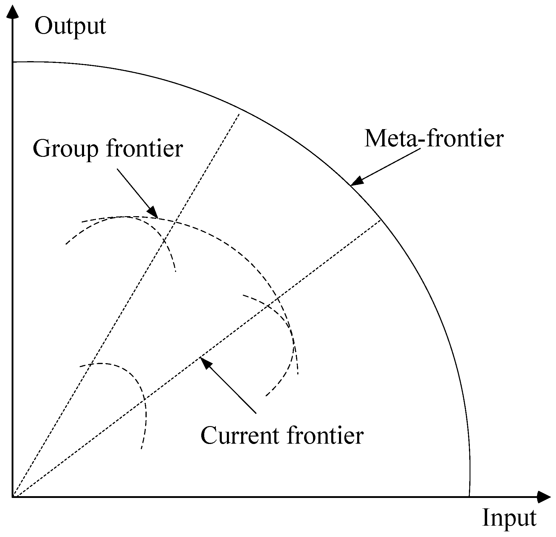
The directional distance function (DDF) is an important tool to measure output and input distances and get the optimal solution based on production theory [22,23]. Hence, DDF was used to measure the optimal solution of the PPS. In this section, meta-frontier and ML index were combined to measure the environmental performance. The concept of meta-frontier was proposed by Hayami [24] to solve error problems of the single production frontier. This model generated a meta-frontier by enveloping three single group frontiers of different groups as shown in Figure 1. Models under group frontier and meta-frontier were all built to measure the environmental performance.
In the model, is the input vector, is the expected output vector and is unexpected output vector. Cities were divided into three groups by two-step clustering as shown in the next chapter. The DMUs were assigned to the same set of technologies, as follows:
The can be defined as follows:
represents the production possible set of the j group under the group frontier or meta-frontier. represents the technology set of the j group under different frontiers. The upper boundary of the is the frontier, so its DDF can be defined as follows:
Its technical efficiency and the relationship between meta-frontier () and group frontier () can be expressed as follows:
Under the frontier, the environmental performance index of a certain type of city is defined in the period from t to t+1. By using directional distance functions, the ML index can be decomposed as follows [20,25]:
where represents the environmental performance change index under the frontier, represents technical efficiency at the time period, represents a technical gap between t and t+1 along the ray from the observation at different time periods, and represent the intertemporal change of efficiency and technology respectively. They indicate the intertemporal change ratio of the actual environmental performance level of a city to the environmental performance level under the production frontier. Additionally, represents the environmental performance level of a city in the t period, represents the level of environmental performance of a city during the period t + 1, represents the environmental performance level of a city in the period t with reference to the t+1 period, and represents the environmental performance level of a city in the period t+1 with reference to the t period.
If , it means that the configuration of reasonable allocation of input and output indicators is optimized. If , it means that the configuration of reasonable allocation of input and output indicators is poor. measures the degree of technological progress. If , it means that the technical level is improved. In details, if , it shows that the city’s environmental performance has been improved. The ML index, the efficiency change index , and the technological progress index , greater than 1 respectively indicate the growth of urban environmental performance, the technological improvement, and the increased distance (the raised efficiency) of the evaluated city from the production frontier. Less than 1 respectively indicates the decline of a city’s environmental performance, technical retrogression, and the reduced distance (the reduced efficiency) of the evaluated city from the production frontier.
3. Empirical Results
In this section, the data from 285 cities in China were clustered into three types using the two-step cluster method to ensure comparability. The urban environmental performances under the meta-frontier and group frontier were both evaluated dynamically to compare cities’ rankings. Additionally, the urban economic growth was compared with the ML growth to identify the true economic achievement when combining both economic and environmental factors.
3.1. Data and Sources
The data used in this paper was collected in the China City Statistical Yearbooks from 2005 to 2013, which provide annual time series of four input and four output variables of 285 cities in China. As the selection of variables should be performed in a scientific, systematic, and rigorous way rather than relying on subjective intentions, this paper therefore selected the input and output variables based on the principles of policy relation, comparability, data availability, and representability. Table 1 shows the selected variables from existing research studies.
It is notable that the number of variables depends on the number of DMUs and only matching between them can get the best results [26]. According to existing research, the number of DMUs should not be less than twice the total number of input and output variables [27]. In this paper, the literature review method was used to choose the input and output variables which refer to environment, economy and society as shown in Table 1. Finally, eight variables were identified including input variables i.e., Labor (X1), Capacity Stock (X2), Water Consumption (X3), Energy Consumption (X4) and output variables i.e., GDP (X5), Industrial Waste Water Emissions (X6), SO2 Emissions (X7), and Dust Emissions (X8). Notably, the variables X6, X7, and X8 are unexpected outputs and means these outputs are negative results of urban economic activities. Figure 2 shows the data structure of the Input-Output variables system. Notably, the number of DMUs far exceeds the number of variables, which meets the principle of variable selection.
In fact, each city is different with respect to economic growth, production technologies, and policy support levels. For example, from the perspective of environmental performance, cities with high production ability which means high energy consumption cannot be compared with cities with low production ability. This indicates that comparison among cities with different levels is inappropriate. Therefore, in this paper, the energy consumption per GDP was used to classify 285 cities into three types which show different technological levels under the group frontier [38]. By two-step clustering using SPSS software, 285 cities in China were partitioned into three clusters, of which the means of the energy consumption per GDP are 0.04, 0.11, and 0.43, respectively. These three types of cities were named low energy intensity, medium energy intensity, and high energy intensity city as shown in Table 2 and Figure 3.
3.2. Environmental Performance under the Meta-Frontier
MAXDEA software was used to calculate the ML index and its decomposition indexes MLEC and MLTC, namely efficiency change (EC) index, and technological change (TC) index below. Among 285 cities, the ML indexes of 166 cities are greater than 1, which indicates that the urban environmental performances of these cities have been improved during the observation period. Table 3 shows the results of ML, EC, and TC indexes under the meta-frontier and group frontier in selected cities with higher and lower results during the period of 2005 to 2013. Within the type of Low and Medium Energy Intensity, cities with the highest growth of urban environmental performance are Hefei and Xiamen, increasing average 30% and 19.9%, respectively. The cities with the highest decrease of urban environmental performance are Pingliang and Yichun, decreasing average 27.1% and 25.8%, respectively. Within the type of High Energy Intensity, the urban environmental performances of all cities decreased averagely while the largest decline was 15.1% in Yangquan and the smallest decline was 0.6% in Shizuishan.
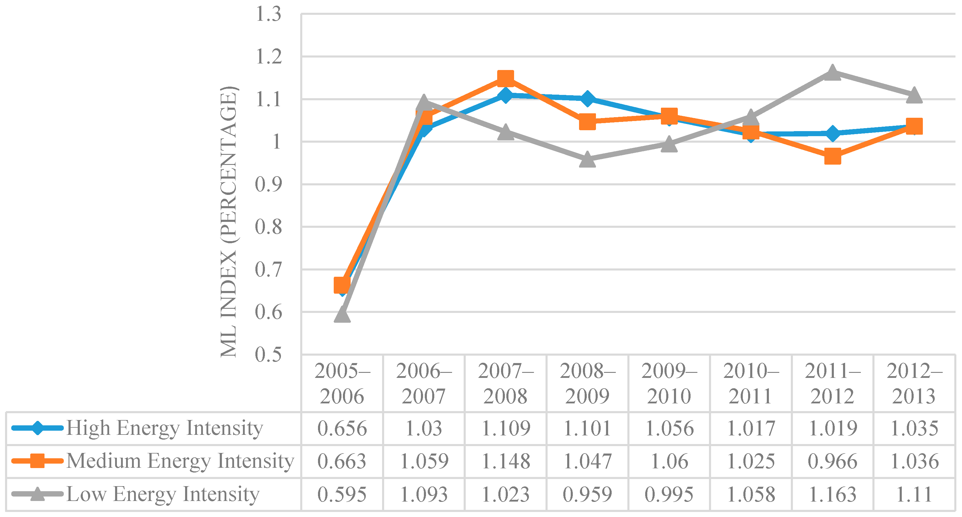
Figure 4 shows the results of the ML indexes in three types of cities between 2005 and 2013. The ML indexes in low energy intensity cities are significantly lower than those in high and medium energy intensity cites which means the improvement of urban environmental performance in low energy intensity cities is insignificant. These results match the practice. For cities consuming smaller energy, the marginal utility of policies related to the environment is weakened. So it is difficult to improve the condition of urban environment significantly. Additionally, towards the end of the Chinese eleventh five-year plan (2006–2010) the urban environmental performance had a substantial increase but during the financial crisis in 2008, the economic recession led to a decline in growth rates, especially in low energy intensity cities.
Table 4 and Figure 5 show the ML index and its decomposition indexes under the meta-frontier. For cities consuming high energy, all three indexes are relatively stable. The means of annual ML indexes were more than 1 from 2005 to 2008, which indicates continued improvement. Then the index kept steady after a slight decrease from 2008 to 2010. The average increase rates of EC and TC were 1.4% and −1% which indicates the EC index had a direct effect on the ML index in general. In 2006, the TC index had a significant increase. The EC index fluctuated around 1. We can see that in the period from 2005 to 2007 and 2010 to 2012, the TC indexes drive the change of the ML index. However, from 2007 to 2009 the ML index was mainly affected by the EC index. In the period of 2011 to 2013, the EC and TC indexes affected the ML index simultaneously.
As for cities consuming medium energy, overall ML indexes remained stable over the period. From 2005 to 2007, the ML index jumped to more than 1 and then this figure remained steady at around 1 after 2007 as Figure 5 shows. However, in 2012 this index soared to 1.036. Table 4 shows the means of EC, TC, and ML, which are 1.003, 0.998, and 1.001. We can see that overall the EC index drove the increase of the ML index. In 2006, the TC index jumped which was driven by the Chinese eleventh five-year plan too because of the trend of innovation. However, in 2008 and 2009 this index declined slightly because the financial crisis led to the decline of the global economy. In conclusion, from 2005 to 2007 and from 2011 and 2013, the ML index was affected by the TC index but from 2006 to 2008 and 2009 to 2011, it was affected by the EC index. In other periods, these two indexes affected the ML simultaneously.
It is clear from the first part of Table 4 and Figure 5 that the environmental performance in low energy-consuming cities fell and the ML indexes were less than 1 in most years. The change percentages of EC, TC, and ML index were −2.6%, 2.4%, and −0.3% respectively which means the EC index resulted in the decline of the ML index. From 2005 to 2008, the EC index experienced an increasing trend and then this figure remained at about 1. However, the TC index experienced fluctuation over that period. In 2008, the TC dropped substantially after the increasing trend between 2005 and 2007. Overall, from 2006 to 2008 and 2009 to 2011, the TC index was the main motivator. From 2011 to 2013, the ML index was affected by the EC index. In other periods, the common influence was the main reason for the change of the ML index.
3.3. Environmental Performance under the Group Frontier
Under the group frontier, the EC, TC, and ML indexes were calculated in 285 cities. It was found that the ML indexes in 185 cities were more than 1, which means the urban environmental performance in these cities rose over the observed period. The right side of Table 3 shows the results of ML, EC, and TC indexes under the group frontier in selected cities. In low energy intensity cities, the environmental condition of Hefei and Shenyang had a great improvement, increasing 32.2% and 20%, respectively. In contrast, Xiaogan and Yaan experienced a falling trend, declining more than 15%. Chongqing and Anyang, which are included in cluster 2, had a significant increase but Liaoyang and Huludao had a significant decrease. Similarly, for cities consuming high energy, the cities with positive performances are Wuhai and Panzhihua whose ML indexes are 1.095 and 1.030 and the city with the worst performance is Jinchang (ML index is 0.985) which means it performed with a decreasing trend for the environmental condition.
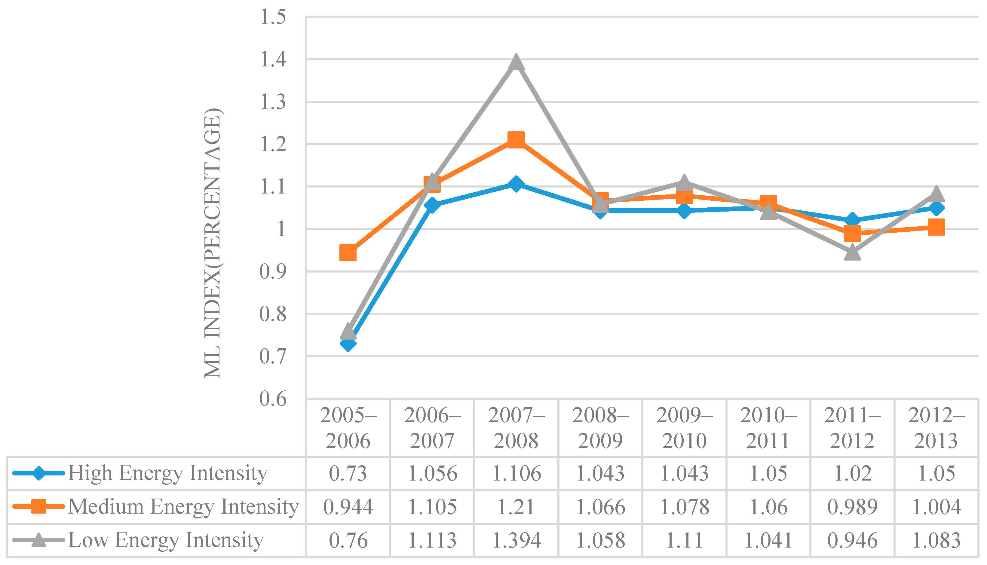
Figure 6 shows changes of the ML index in three types of cities under the group frontier. It is clear from the figure that the trends of the three lines are similar. The environmental performances of most cites improved significantly. For low energy intensity cities, in 2008 the mean of environmental performance dropped considerably after a noticeable rise from 2005 to 2007 and in 2009 there was a slight increase. After 2009, the environment performances of these three kinds of cities were all declined and the fastest fall occurred in low energy intensity cities.
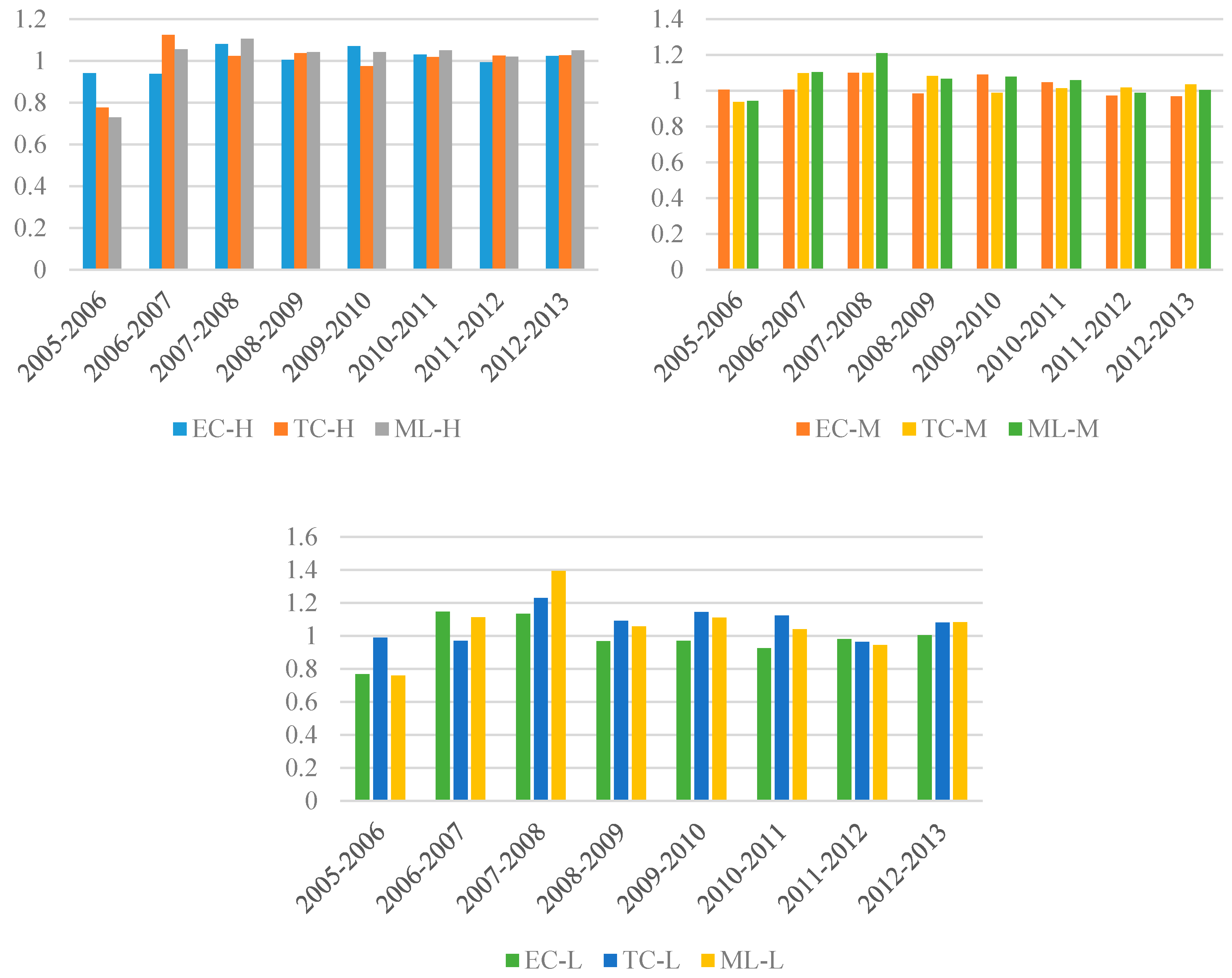
Under the group frontier, the mean of the ML index in high energy intensity cities is 1.012 and ML indexes are more than 1 in most observed periods. This trend means the environmental performance in this kind of city experienced an increase. The EC and TC indexes increased by 1.1% and 1% averagely and they all contributed to the growth of the ML index. It is clear from Table 4 and Figure 7 that from 2005 to 2009 the TC index increased considerably which means promotion of the technological level. Then this index declined to 0.975 which means a technological recession. However, from 2011 the index began to rise again. As for the EC index, it experienced a fluctuating trend during the period but overall it increased. In conclusion, from 2005 to 2007 the TC index contributed to the change of the ML index. From 2007 to 2009 and from 2010 to 2012 the EC indexes were the main driver. In others years, the TC index and EC index influenced the ML index together.
The bottom part of Table 4 shows that overall the ML index was relatively stable and the average increased by 5.7% in medium energy intensity cities under the group frontier. The EC index and the TC index rose by 2.2% and 3.4% which means they all played a positive role. Figure 7 shows the change of these three indexes in medium energy intensity cities under the group frontier. From 2006 to 2007, the TC index went up significantly to 1.098. Then it experienced a slight decline. After that, this figure began to increase again. As for the EC index, prior to 2008 it remained with an increasing trend rising from 1.007 to 1.1 but in 2009 it had a considerable drop. Then it still fluctuated around 1. In conclusion, from 2005 to 2007 and from 2011 to 2013, the TC index drove the change of the ML index and from 2009 to 2011 the EC index was the driver. During other periods, they both contributed to the fluctuation of the ML index.
Finally, in low energy intensity cities, the ML index fluctuated during the period but the mean (1.061) still remained increased, because the mean of the TC index increased by 7.4% although the EC index decreased by 1.3%. In detail, as it is shown in Figure 7, between 2005 and 2007 the TC index dropped. Interestingly, in 2008 this index increased which drove the rethinking of the influence of the financial crisis. However, the EC index did not jump up. Then the TC index experienced a slight fluctuation. As for the EC index, between 2005 and 2007 and between 2012 and 2013 it rose but in other periods, this index experienced a decline. In conclusion, in most years the ML indexed was affected by the TC index and the EC index.
3.4. Comparison between Different Frontiers
Under different frontiers, the results are compared in Figure 8 which shows the average ML indexes in high, medium, and low energy intensity cities. It is clear that the trends of the ML index under the meta-frontier and group-frontier are similar. Howeber, in most periods the ML index under the group frontier was higher than that under the meta-frontier in different kinds of cities. This means the environmental performance under the group frontier was overestimated and in the medium energy intensity group, this trend was more obvious. Apart from 2008, the gap between the meta-frontier and group frontiers was smallest in the low energy intensity group. This is because the technological levels in this kind of city were better. Different cities hold different technological levels, so the optimal sets of technology in different clusters are different which present different group frontiers. Under the group frontier, the highest average ML index occurred in the high energy intensity group.
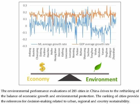
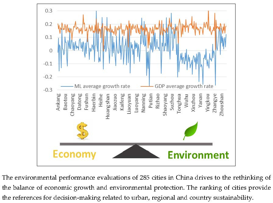
3.5. Comparison between the ML Index and GDP
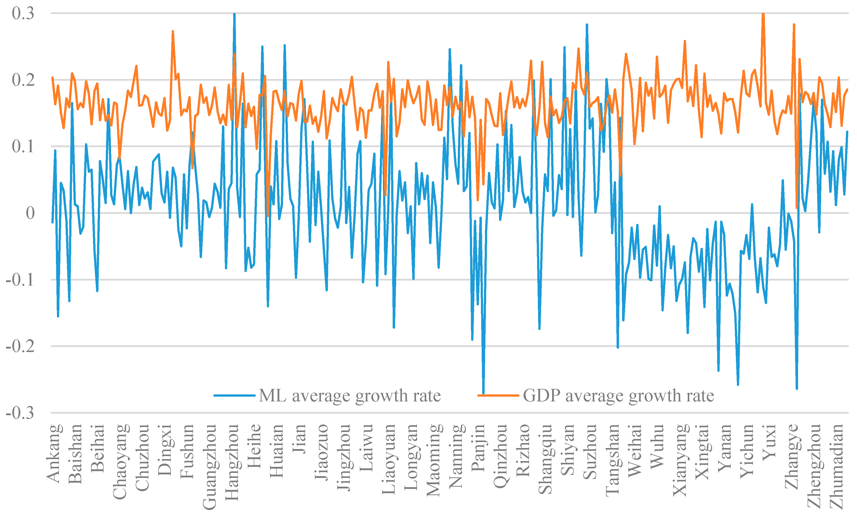
GDP has been the main indicator used to evaluate economic growth of a city for many years. In this section, the relationship between GDP growth and the ML index growth is compared. Figure 9 compares the ML average growth rate with the GDP average growth rate over the period from 2005 to 2013 in some cities. The GDP growth rates of each city fluctuated between 0 and 0.3 which means the economic gaps between cities were not significant during the period from the perspective of the GDP in all 285 cities. Yet the ML index growth rates of these cities were between −0.3 and 0.3 which means the environmental performances gaps between cities were more significant. Additionally, in some cities such as Panjin, Yanan, Yichun, and Zhangye, the trends of GDP growth and ML growth were totally opposite which drove to rethinking on the evaluation of urban development.
4. Discussions
Based on the results, some interesting issues are worthy of further discussions as follows:
- (1)
- The ML indexes in 166 cities under the meta-frontier and 185 cities under the group frontier are more than 1, which indicates that the urban environmental performances in these cities were improved during the observation period. In most years the ML indexes under the group frontier were higher than that under the meta-frontier in different types of cities. This overestimation under the group frontier for high energy intensity cities is more obvious. Because production technologies in this type of city were not advanced, they had a lower technological frontier. This also means it is difficult to match the group frontier to the meta-frontier by improving the technological efficiency. However, narrowing the technology gap between different types of cities is a more efficient method to improve the urban environmental performance in China.
- (2)
- It is notable that the EC and TC indexes of cities with higher ML growth also remained with an increasing trend basically and the gap between these two indexes was smaller relatively. This indicates in these cities that resource allocation and structure were relatively reasonable, and technological innovation abilities were stronger. However, in these cities with decreasing environmental performances, at least one of its EC or TC index remained at negative growth which means the resource allocation and structure were unreasonable and the technological levels were lower. Thus, the balance between efficient improvement and technological promotion is significant for the overall increase in environmental performance.
- (3)
- Economic policies and crisis have important influences on urban environmental performances. For example, in 2006 and 2012 the ML index had a significant increase. In this period, China published the Chinese eleventh five-year plan (2006–2010) and Environmental government policies such as “Air Pollution Control Action Plan” and “PM2.5 Monitoring”. All of these policies related to industrial structure and resources conservation promoting technological innovation vigorously. The findings are partly in line with previous research [39], government economic plans can lead to a significant change of the environmental situation. Additionally, in 2008 the ML index and its decomposed EC and TC experienced a decreasing trend when the global financial crisis occurred. Thus, strategic policies and huge crises should be considered as external factors when we evaluate environmental performance.
- (4)
- In most cities, the ML growth rates were significantly smaller than GDP growth rates and even totally opposite trends existed between these two indexes. This indicates it is not enough to evaluate the economic development of a city only by GDP. The energy consumption and the environmental performance are also important indicators to evaluate urban development from the sustainable perspective. So it is necessary to rethink the achievement of urban development by combining economy-related indicators and environment-related indicators.
5. Conclusions
Under the goals of sustainable development, environmental performance evaluation of a city needs to be continually improved and expanded. In this study, the research scope was extended to 285 prefecture-level cities, which expands traditional provincial analysis. A dynamic evaluation model was built to assess urban environmental performance over the period of 2005 to 2013. Additionally, the combination of ML index with frontier analysis was used to assess the change trends of urban environmental performance. Thedecomposition indexes efficiency change (EC) index and the technological change (TC) index were also used to identify the main reasons for different trends. Importantly, 285 cities were divided into three categories by the method of two-step clustering which increases the validity and the accuracy of the data comparison.
According to empirical results, we found that the ML indexes were overestimated under the group frontier compared with those under the meta-frontier. For evaluation units with obvious clustering features, ML analysis considering meta-frontier is a more efficient method to solve problems. In addition, the growth rates of urban environmental efficiency were smaller in low energy intensity cities under both two frontiers. This indicates the marginal effects of environmental policies were weakened in this kind of city. In contrast, the increases of environmental performance were relatively larger in medium and high energy intensity cities. To solve differences between clusters, different policies relating to sustainable development should be considered to achieve city, region, and country sustainability. What is more, the gap between the ML index and GDP drives rethinking of the evaluation method on city development. This paper contributes to both method improvement and practical understanding by evaluating the environment in 285 cities from different perspectives.
Additionally, some specific suggestions are provided below. Narrowing the technological differences between the frontiers is an important way to improve the overall environmental performance. In detail, establishing an effective cooperation mechanism between different kinds of cities could narrow the differences and achieve a win-win situation to improve urban and even regional sustainability. Besides, the growth of the environmental performance (ML index) is affected by both technological change and efficiency change. All methods increasing desirable outputs and decreasing undesirable outputs could achieve improvement of the environment. For example, technological innovation is one of the most important ways to enhance environmental performance. Advanced technologies not only decrease the input, energy consumption but the undesirable output, emissions. In conclusion, support for research and policies related to technological innovation are necessary to narrow regional gaps of environmental performances and achieve overall sustainability for the government. For companies promoting innovation culture, increasing the intensity of technological research and responding to policies are all efficient ways to gain positive environmental outputs.
Acknowledgements
This research was supported by the National Natural Science Foundation of China (NSFC) (Grant No. 71390522, NO. 71671053). The work described in this paper was also funded by the National Key R&D Program of China (No. 2016YFC0701808) and the Twelfth Five-Year National Science and Technology R&D Program of China (No. 2014BAL05B06).
Conflicts of Interest
The authors declare no conflict of interest.
References
- Wigginton, N.S.; Fahrenkamp-Uppenbrink, J.; Wible, B. Cities are the future. Science 2016, 352, 904–905. [Google Scholar] [CrossRef] [PubMed]
- American Association for the Advancement of Science. Rise of the city. Science 2016, 352, 906–907. [Google Scholar] [CrossRef]
- Henderson, J.V.; Venables, A.J.; Regan, T. Building functional cities. Science 2016, 352, 946–947. [Google Scholar] [CrossRef] [PubMed] [Green Version]
- Hartig, T.; Kahn, P.H. Living in cities, naturally. Science 2016, 352, 938–940. [Google Scholar] [CrossRef] [PubMed]
- Färe, R.; Grosskopf, S.; Pasurka, C. The effect of environmental regulations on the efficiency of electric utilities: 1969 versus 1975. Appl. Econ. 1989, 21, 225–235. [Google Scholar] [CrossRef]
- Epstein, M.J.; Wisner, P.S. Using a balanced scorecard to implement sustainability. Environ. Qual. Manag. 2001, 11, 1–10. [Google Scholar] [CrossRef]
- Corbett, C.J.; Pan, J.N. Evaluating environmental performance using statistical process control techniques. Eur. J. Oper. Res. 2002, 139, 68–83. [Google Scholar] [CrossRef]
- Tam, V.W.Y.; Tam, C.M.; Zeng, S.X. Environmental performance measurement indicators in construction. Build. Environ. 2006, 41, 164–173. [Google Scholar] [CrossRef]
- Awasthi, A.; Chauhan, S.S.; Goyal, S.K. A fuzzy multicriteria approach for evaluating environmental performance of suppliers. Int. J. Prod. Econ. 2010, 126, 370–378. [Google Scholar] [CrossRef]
- Hasanali, A.; Abbas, N.A.; Hossein, N. Environmental Performance Evaluation Based on Fuzzy Logic. In Proceedings of the International Conference on Social Science and Humanity, Singapore, 26 February 2011; International Association of Computer Science and Information Technology Press: Singapore, 2011. [Google Scholar]
- Kammen, D.M.; Sunter, D.A. City-integrated renewable energy for urban sustainability. Science 2016, 352, 922–928. [Google Scholar] [CrossRef] [PubMed]
- Zucaro, A.; Ripa, M.; Mellino, S. Urban resource use and environmental performance indicators. An application of decomposition analysis. Ecol. Indic. 2014, 47, 16–25. [Google Scholar] [CrossRef]
- Frank, A.G.; Dalle, M.N.; Gerstlberger, W. An integrative environmental performance index for benchmarking in oil and gas industry. J. Clean. Prod. 2016, 133, 1190–1203. [Google Scholar] [CrossRef]
- Xue, X.L.; Wu, H.Q.; Zhang, X.L. Measuring energy consumption efficiency of the construction industry: The case of China. J. Clean. Prod. 2015, 107, 509–515. [Google Scholar] [CrossRef]
- Aparicio, J.; Barbero, J.; Kapelko, M. Testing the consistency and feasibility of the standard Malmquist-Luenberger index: Environmental productivity in world air emissions. J. Environ. Manag. 2017, 196, 148–160. [Google Scholar] [CrossRef] [PubMed]
- He, Y.; Xie, H.; Fan, Y.; Wang, W.; Xie, X. Forested land use efficiency in China: Spatiotemporal patterns and influencing factors from 1999 to 2010. Sustainability 2016, 8, 772. [Google Scholar] [CrossRef]
- Du, M.; Wang, B.; Wu, Y. Sources of China’s economic growth: An empirical analysis based on the BML index with green growth accounting. Sustainability 2014, 6, 5983–6004. [Google Scholar] [CrossRef]
- Hong, H.; Xie, D.; Liao, H.; Tu, B.; Yang, J. Land use efficiency and total factor productivity—Distribution dynamic evolution of rural living space in Chongqing, China. Sustainability 2017, 9, 444. [Google Scholar] [CrossRef]
- Zhang, J.; Fang, H.; Peng, B.; Wang, X.; Fang, S. Productivity growth-accounting for undesirable outputs and its influencing factors: The case of China. Sustainability 2016, 8, 1166. [Google Scholar] [CrossRef]
- Oh, D. A global Malmquist-Luenberger productivity index. J. Product. Anal. 2010, 34, 183–197. [Google Scholar] [CrossRef]
- Färe, R.; Grosskopf, S.; Pasurka, C.A. Environmental production functions and environmental directional distance functions. Energy 2007, 32, 1055–1066. [Google Scholar] [CrossRef]
- Färe, R.; Grosskopf, S. Theory and application of directional distance functions. J. Product. Anal. 2000, 13, 93–103. [Google Scholar] [CrossRef]
- Chung, Y.H.; Färe, R.; Grosskopf, S. Productivity and undesirable outputs: A directional distance function approach. J. Environ. Manag. 1997, 51, 229–240. [Google Scholar] [CrossRef]
- Hayami, Y. Sources of agricultural productivity gap among selected countries. Am. J. Agric. Econ. 1969, 51, 564–575. [Google Scholar] [CrossRef]
- Färe, R.; Grosskopf, S.; Lindgren, B. Productivity Developments in Swedish Hospitals: A Malmquist Output Index Approach; Springer: Berlin, Germany, 1994; pp. 227–235. [Google Scholar]
- Wang, K.; Yu, S.; Zhang, W. China’s regional energy and environmental efficiency: A DEA window analysis based dynamic evaluation. Math. Comput. Model. 2013, 58, 1117–1127. [Google Scholar] [CrossRef]
- Hu, J.L.; Chang, M.C.; Tsay, H.W. The congestion total-factor energy efficiency of regions in Taiwan. Energy Policy 2017, 110, 710–718. [Google Scholar] [CrossRef]
- Meng, F.Y.; Fan, L.W.; Zhou, P. Measuring environmental performance in China’s industrial sectors with non-radial DEA. Math. Comput. Model. 2013, 58, 1047–1056. [Google Scholar] [CrossRef]
- He, F.; Zhang, Q.; Lei, J. Energy efficiency and productivity change of China’s iron and steel industry: Accounting for undesirable outputs. Energy Policy 2013, 54, 204–213. [Google Scholar] [CrossRef]
- Jin, J.; Zhou, D.; Zhou, P. Measuring environmental performance with stochastic environmental DEA: The case of APEC economies. Econ. Model. 2014, 38, 80–86. [Google Scholar] [CrossRef]
- Chen, S.; Golley, J. Green productivity growth in China’s industrial economy. Energy Econ. 2014, 44, 89–98. [Google Scholar] [CrossRef]
- Genovese, A.; Lenny, K.S.; Kumar, N. Exploring the challenges in implementing supplier environmental performance measurement models: A case study. Prod. Plan. Control 2014, 25, 1198–1211. [Google Scholar] [CrossRef]
- Silva, D.A.L.; Lahr, F.A.R.; Varanda, L.D. Environmental performance assessment of the melamine-urea-formaldehyde (MUF) resin manufacture: A case study in Brazil. J. Clean. Prod. 2015, 96, 299–307. [Google Scholar] [CrossRef]
- BaI, Y.; Deng, X.; Zhang, Q. Measuring environmental performance of industrial sub-sectors in China: A stochastic metafrontier approach. Phys. Chem. Earth 2017, 101, 3–12. [Google Scholar] [CrossRef]
- Li, K.; Lin, B. Impact of energy conservation policies on the green productivity in China’s manufacturing sector: Evidence from a three-stage DEA model. Appl. Energy 2016, 168, 351–363. [Google Scholar] [CrossRef]
- Beltrán-Esteve, M.; Picazo-Tadeo, A.J. Assessing environmental performance in the European Union: Eco-innovation versus catching-up. Energy Policy 2017, 104, 240–252. [Google Scholar] [CrossRef]
- Zuo, X.; Hua, H.; Dong, Z. Environmental Performance Index at the Provincial Level for China 2006–2011. Ecol. Indic. 2017, 75, 48–56. [Google Scholar] [CrossRef]
- Huang, Y.J.; Chen, K.H.; Yang, C.H. Cost efficiency and optimal scale of electricity distribution firms in Taiwan: An application of metafrontier analysis. Energy Econ. 2010, 32, 15–23. [Google Scholar] [CrossRef]
- Zhou, D.; Wang, Q.; Su, B.; Zhou, P.; Yao, L. Industrial energy conservation and emission reduction performance in China: A city-level nonparametric analysis. Appl. Energy 2016, 166, 201–209. [Google Scholar] [CrossRef]
Figure 1.
Concept of the meta-frontier Malmquist–Luenberger productivity index.

Figure 2.
Data structure of the Input-Output variable system.
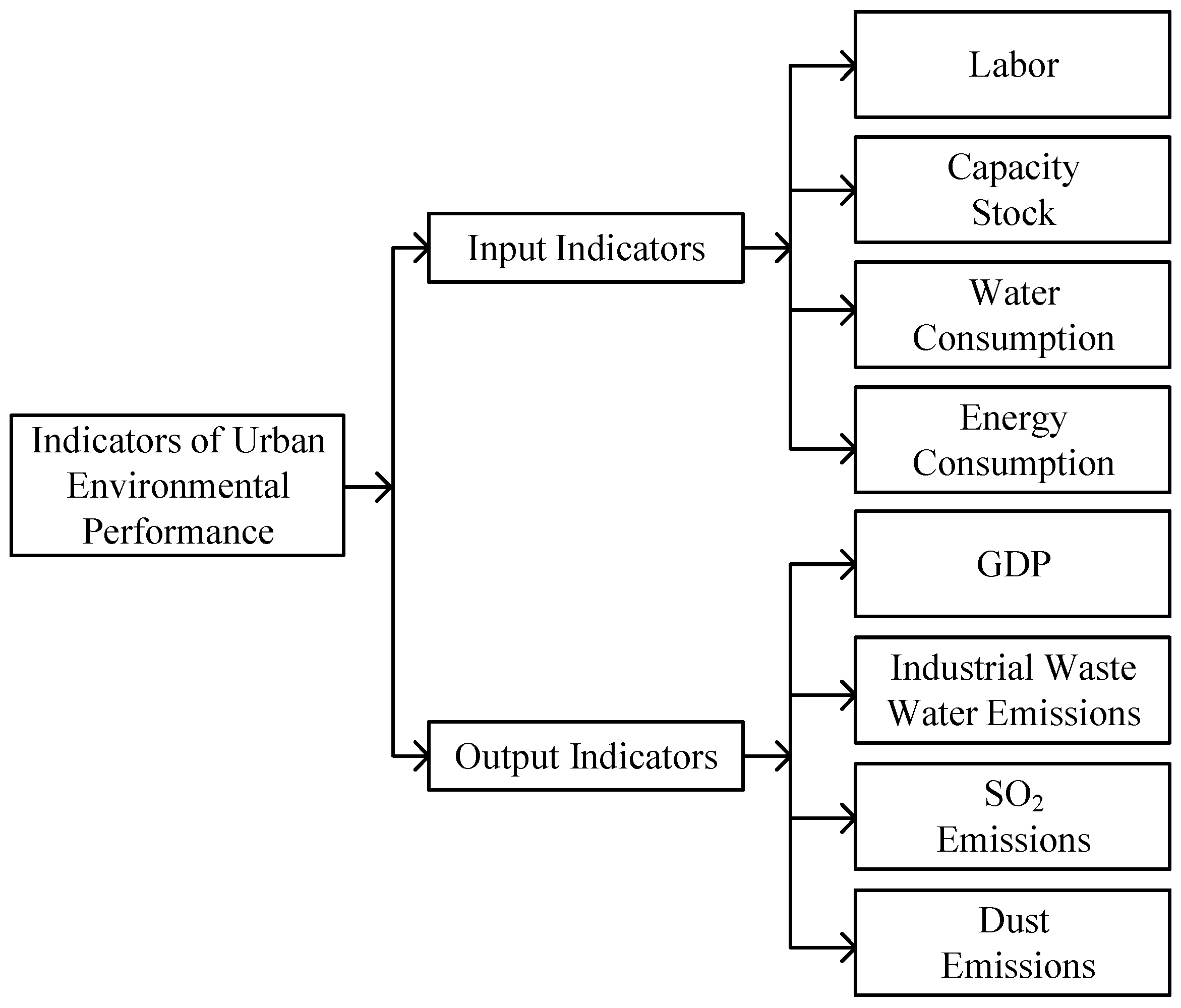
Figure 3.
Distribution of clustered cities.
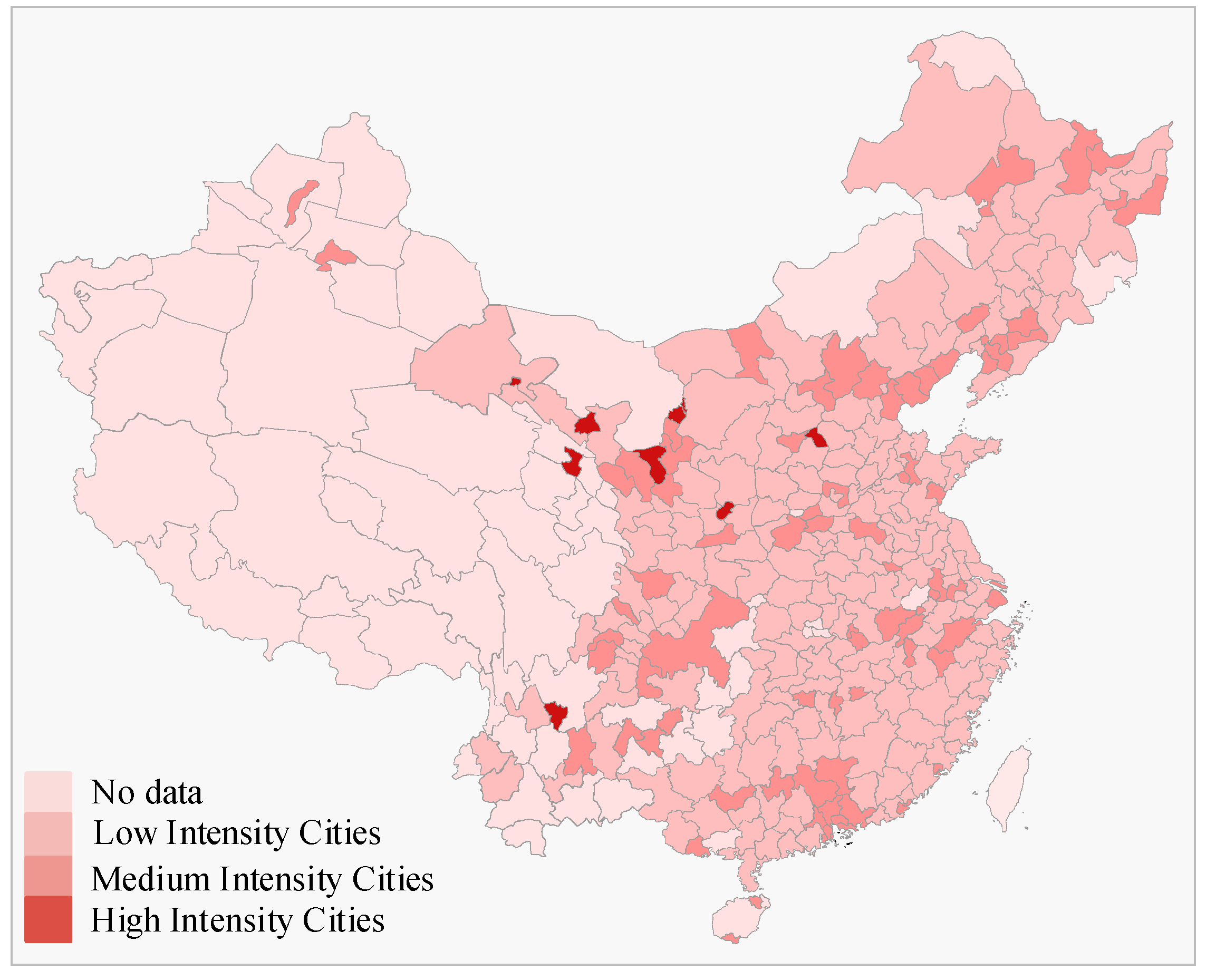
Figure 4.
ML index of three classifications under the meta-frontier.

Figure 5.
Indexes in three kinds of cities under the meta-frontier.
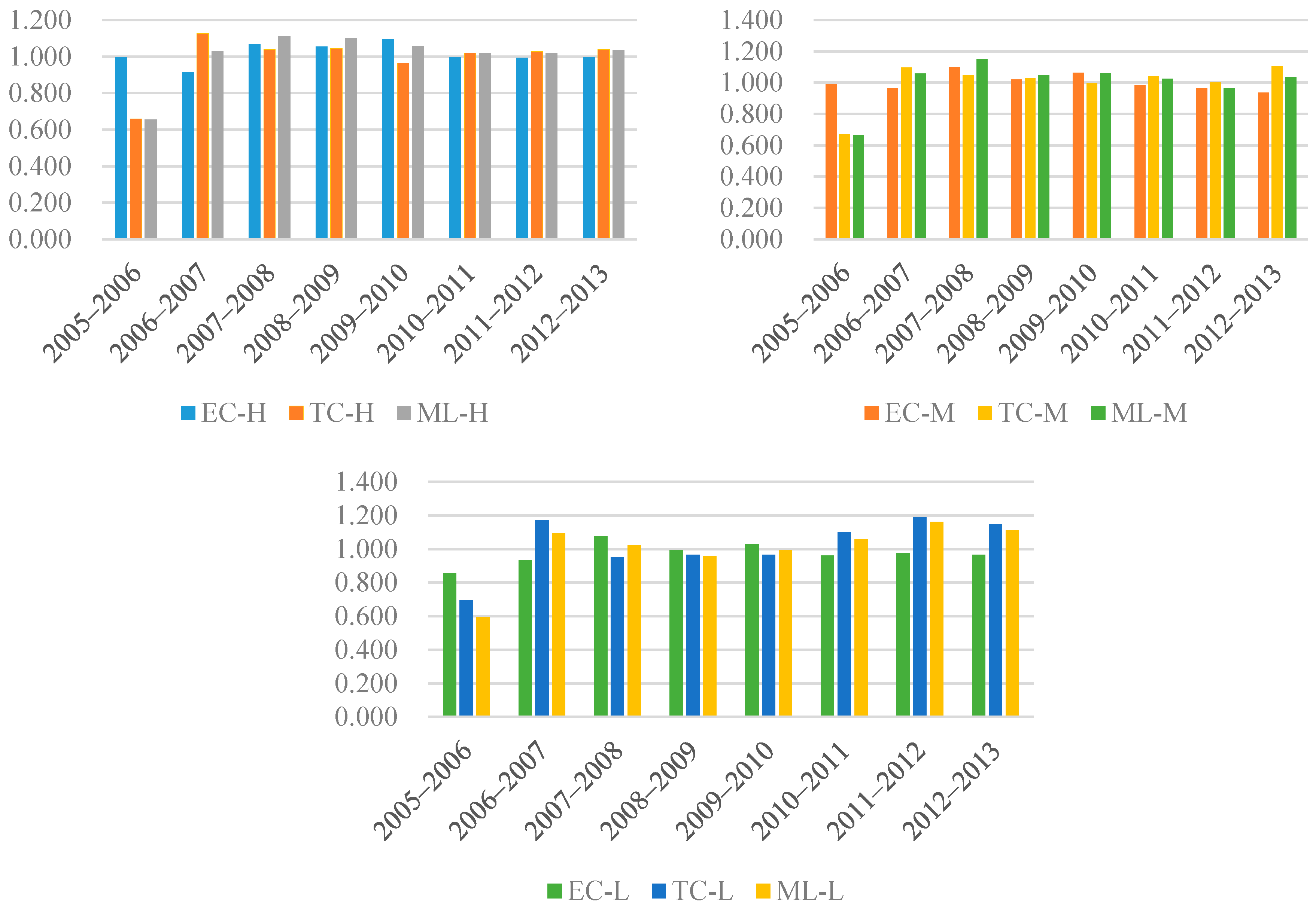
Figure 6.
ML index of three classifications under the group-frontier.

Figure 7.
Indexes in three kinds of cities under the group-frontier.

Figure 8.
The ML index under different technological frontiers.
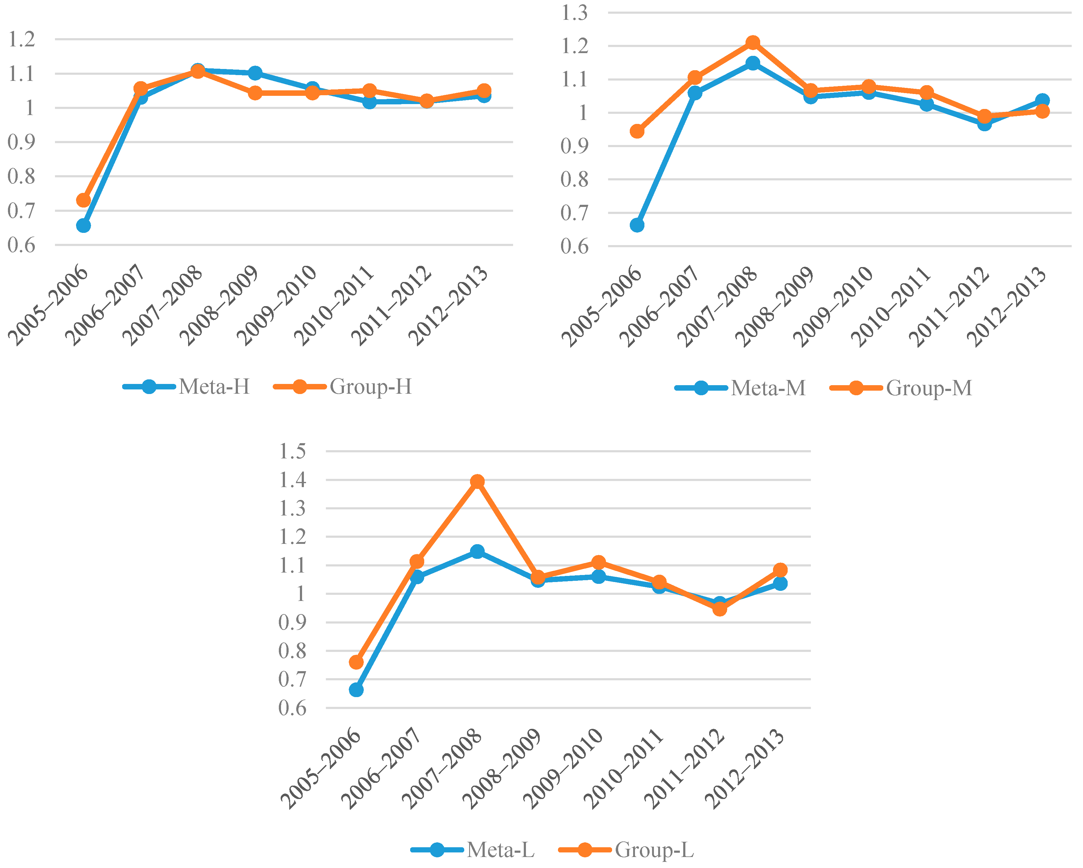
Figure 9.
The gap between the ML index and GDP.


Table 1.
Variables identification.
| Literatures | X1 | X2 | X3 | X4 | X5 | X6 | X7 | X8 |
|---|---|---|---|---|---|---|---|---|
| Wang, 2013 [26] | √ | √ | √ | √ | √ | |||
| Meng, 2013 [28] | √ | √ | √ | |||||
| He, 2013 [29] | √ | √ | ||||||
| Jin, 2014 [30] | √ | √ | √ | |||||
| Chen, 2014 [31] | √ | √ | √ | |||||
| Genovese, 2014 [32] | √ | √ | ||||||
| Silva, 2015 [33] | √ | √ | ||||||
| Bai, 2016 [34] | √ | √ | √ | |||||
| Li, 2016 [35] | √ | √ | √ | |||||
| Beltrán-Esteve, 2017 [36] | √ | √ | √ | √ | ||||
| Zuo, 2017 [37] | √ | √ | √ | √ |
Table 2.
Clustering results of cities.
| Types | Clusters | Mean | Number | Cities (Partly) |
|---|---|---|---|---|
| Low Energy Intensity | 1 | 0.04 | 198 | Ankang, Baise, Bayanzhuoer, Bengbu, Baicheng, Bazhong, Binzhou, Baoji, Cangzhou, Baoding |
| Medium Energy Intensity | 2 | 0.11 | 78 | Anqing, Baiyin, Anshun, Baotou, Anshan, Anyang, Changzhou, Benxi, Beijing, Quzhou |
| High Energy Intensity | 3 | 0.43 | 9 | Jinchang, Jiayuguan, Panzhihua, Shizuishan, Tongchuan, Wuhai, Xining, Yangquan, Zhongwei |
Table 3.
ML index under two kinds of frontier (Partly).
| City-Meta | Cluster | EC | TC | ML | City-Group | Cluster | EC | TC | ML |
|---|---|---|---|---|---|---|---|---|---|
| Hefei | 1 | 1.142 | 1.138 | 1.300 | Hefei | 1 | 1.142 | 1.157 | 1.321 |
| Songyuan | 1 | 1.199 | 1.071 | 1.283 | Shenyang | 1 | 1.098 | 1.185 | 1.301 |
| Huanggang | 1 | 1.166 | 1.074 | 1.252 | Songyuan | 1 | 1.237 | 1.040 | 1.287 |
| Huhehaote | 1 | 1.172 | 1.067 | 1.250 | Huhehaote | 1 | 1.172 | 1.073 | 1.258 |
| Shenyang | 1 | 1.098 | 1.137 | 1.249 | Huanggang | 1 | 1.166 | 1.072 | 1.250 |
| Pingliang | 1 | 0.797 | 0.915 | 0.729 | Pingliang | 1 | 0.797 | 0.900 | 0.717 |
| Xiamen | 2 | 1.118 | 1.073 | 1.199 | Chongqing | 2 | 1.050 | 1.144 | 1.201 |
| Chongqing | 2 | 1.119 | 1.046 | 1.170 | Anyang | 2 | 1.126 | 1.056 | 1.189 |
| Zhengzhou | 2 | 1.124 | 1.039 | 1.168 | Nanjing | 2 | 1.124 | 1.033 | 1.162 |
| Nanjing | 2 | 1.109 | 1.020 | 1.130 | Leshan | 2 | 1.083 | 1.071 | 1.161 |
| Haikou | 2 | 1.034 | 0.996 | 1.130 | Baotou | 2 | 1.074 | 1.075 | 1.155 |
| Yichun | 2 | 0.992 | 0.748 | 0.742 | Liangyang | 2 | 0.810 | 1.022 | 0.828 |
| Shizuishan | 3 | 1.006 | 0.989 | 0.994 | Shizuishan | 3 | 0.984 | 1.155 | 1.136 |
| Panzhihua | 3 | 1.076 | 0.918 | 0.988 | Wuhai | 3 | 1.021 | 1.072 | 1.095 |
| Jiayuguan | 3 | 0.991 | 0.992 | 0.982 | Panzhihua | 3 | 1.014 | 1.016 | 1.030 |
| Yangquan | 3 | 0.902 | 0.940 | 0.849 | Tongchuan | 3 | 1.000 | 1.000 | 1.000 |
| Jinchang | 3 | 0.947 | 0.934 | 0.884 | Xining | 3 | 1.005 | 0.994 | 0.999 |
| Tongchuan | 3 | 0.999 | 0.926 | 0.925 | Jinchang | 3 | 0.995 | 0.989 | 0.985 |
Abbreviations: ML: Malmquist-Luenberger index, EC: efficiency change index of ML, TC: technological change index of ML, City-Meta: cities’ indexes under the meta-frontier, City-Group: cities’ indexes under the group frontier.
Table 4.
Indexes under two kinds of frontiers.
| City | Index | 2005–2006 | 2006–2007 | 2007–2008 | 2008–2009 | 2009–2010 | 2010–2011 | 2011–2012 | 2012–2013 | Mean |
|---|---|---|---|---|---|---|---|---|---|---|
| HIGH–meta | EC | 0.995 | 0.914 | 1.067 | 1.054 | 1.096 | 0.997 | 0.993 | 0.996 | 1.014 |
| TC | 0.659 | 1.126 | 1.039 | 1.045 | 0.964 | 1.019 | 1.027 | 1.039 | 0.990 | |
| ML | 0.656 | 1.030 | 1.109 | 1.101 | 1.056 | 1.017 | 1.019 | 1.035 | 1.004 | |
| MEDIUM–meta | EC | 0.989 | 0.966 | 1.098 | 1.020 | 1.063 | 0.984 | 0.966 | 0.937 | 1.003 |
| TC | 0.670 | 1.096 | 1.046 | 1.026 | 0.997 | 1.042 | 1.000 | 1.105 | 0.998 | |
| ML | 0.663 | 1.059 | 1.148 | 1.047 | 1.060 | 1.025 | 0.966 | 1.036 | 1.001 | |
| LOW–meta | EC | 0.855 | 0.933 | 1.076 | 0.993 | 1.030 | 0.962 | 0.976 | 0.966 | 0.974 |
| TC | 0.696 | 1.171 | 0.952 | 0.966 | 0.967 | 1.099 | 1.192 | 1.149 | 1.024 | |
| ML | 0.595 | 1.093 | 1.023 | 0.959 | 0.995 | 1.058 | 1.163 | 1.110 | 0.997 | |
| HIGH–group | EC | 0.941 | 0.938 | 1.081 | 1.005 | 1.071 | 1.031 | 0.994 | 1.023 | 1.011 |
| TC | 0.776 | 1.125 | 1.023 | 1.038 | 0.975 | 1.018 | 1.026 | 1.027 | 1.001 | |
| ML | 0.73 | 1.056 | 1.106 | 1.043 | 1.043 | 1.05 | 1.02 | 1.05 | 1.012 | |
| MEDIUM–group | EC | 1.007 | 1.006 | 1.1 | 0.984 | 1.091 | 1.047 | 0.972 | 0.969 | 1.022 |
| TC | 0.937 | 1.098 | 1.1 | 1.083 | 0.989 | 1.013 | 1.018 | 1.036 | 1.034 | |
| ML | 0.944 | 1.105 | 1.21 | 1.066 | 1.078 | 1.06 | 0.989 | 1.004 | 1.057 | |
| LOW–group | EC | 0.768 | 1.147 | 1.134 | 0.968 | 0.97 | 0.927 | 0.982 | 1.003 | 0.987 |
| TC | 0.99 | 0.971 | 1.23 | 1.092 | 1.145 | 1.124 | 0.964 | 1.08 | 1.074 | |
| ML | 0.76 | 1.113 | 1.394 | 1.058 | 1.11 | 1.041 | 0.946 | 1.083 | 1.061 |
© 2018 by the authors. Licensee MDPI, Basel, Switzerland. This article is an open access article distributed under the terms and conditions of the Creative Commons Attribution (CC BY) license (http://creativecommons.org/licenses/by/4.0/).
Share and Cite
MDPI and ACS Style
Wang, L.; Xue, X.; Shi, Y.; Wang, Z.; Ji, A. A Dynamic Analysis to Evaluate the Environmental Performance of Cities in China. Sustainability 2018, 10, 862. https://doi.org/10.3390/su10030862
AMA Style
Wang L, Xue X, Shi Y, Wang Z, Ji A. A Dynamic Analysis to Evaluate the Environmental Performance of Cities in China. Sustainability. 2018; 10(3):862. https://doi.org/10.3390/su10030862
Chicago/Turabian StyleWang, Luqi, Xiaolong Xue, Yue Shi, Zeyu Wang, and Ankang Ji. 2018. "A Dynamic Analysis to Evaluate the Environmental Performance of Cities in China" Sustainability 10, no. 3: 862. https://doi.org/10.3390/su10030862
Note that from the first issue of 2016, this journal uses article numbers instead of page numbers. See further details here.