A 10-Year Statistical Analysis of Heavy Metals in River and Sediment in Hengyang Segment, Xiangjiang River Basin, China

Abstract

Heavy metal elements in water and surface sediments were characterized in Hengyang river segment in Xiangjiang River basin, one of China’s most important heavy metal control and treatment region. Data of heavy metal monitoring results in water and sediment for 10 years were acquired from an environmental monitoring program in the main channel of the studied area. Descriptive and exploratory statistical procedures were performed to reveal the characteristics of the sample distributions of heavy metal elements. The sample distributions of heavy metal elements were largely skewed right. Data censoring and too severe rounding in the water monitoring data were identified to have caused discretization in the sample distributions. Temporal and spatial characteristics of the data sets were addressed. The chromium (Cr) in the sediment possessed unique behavior, and this could be caused by a rapid deposition and releasing process.

1. Introduction

A river forms an environmental system that is both a sink and a source for heavy metal elements, as well as a carrier for the transportation of these elements. Heavy metal elements in fluvial systems are known for their potential toxicity and ecotoxicity. These elements, including chromium (Cr), manganese (Mn), copper (Cu), zinc (Zn), arsenic (As), cadmium (Cd), mercury (Hg), and lead (Pb), are introduced into rivers by natural processes such as weathering and atmospheric deposition, and more importantly, via anthropogenic discharges from mining and smelting activities [1,2,3,4]. The control and treatment of heavy metal pollution in river and sediment has long been a serious campaign in most nations with intensive smelting activities.

In China, heavy metal contamination in rivers is of great concern to ministration authorities, as well as the public. The Xiangjiang River basin, which is one of the most distinguishable heavy metal influenced areas in China, has drawn nationwide attention and was designated as the first and so far the largest region under the national heavy metal control and treatment plan in China [5]. Much more efforts are still required in this region to achieve a desirable outcome in the control and treatment of heavy metal contamination.

The fundamental step to the control and treatment of heavy metal contamination is to understand the status quo of contamination, which normally requires drawing information from environmental monitoring data. The statistical analysis serves as a conventional and the most prevalent empirical approach to the characterization and exploration of the data. A variety of statistical procedures were used by environmental and geochemical researchers to reveal characteristics and structures within the data, such as outlier identification, correlation analysis, principal component analysis (PCA), factor analysis (FA), and regression modeling [1,6,7,8,9,10,11]. Generally, the first step in statistical data analysis is to perform descriptive and exploratory statistical procedures that focus on single-variable data analysis, which helps one to gain a global understanding of the data and subsequently avails unbiased design and interpretation of further data analyzing procedures. However, with the popularity of statistical data analysis in environmental studies, descriptive and exploratory statistical procedures have been implemented with little consideration in a growing amount of research. Some researchers tend to be result-driven and simply enter popular statistical analysis procedures with collected data, thus neglecting the importance of a careful characterization of the data, as well as a proper selection of methods to approach them. The improper implementation of these basic procedures induces the risks of misleading the interpretation of data and violating important statistical assumptions [12].

In this study, data on heavy metals of both river water and surface sediment in a 10-year monitoring program in Hengyang segment, a typical area in the Xiangjiang River basin under severe heavy metal influence, is being statistically characterized. The aim of this study is to (i) properly present the samples of heavy metals in both the water and the sediment; and (ii) discover the underlying features in the sample distributions.

2. Materials and Methods

2.1. Description of the Research Area

Xiangjiang River runs northward through Hunan province—the world-famous “land of nonferrous metals”—as the second largest tributary to Yangtze River in China. Hengyang is the second prefecture-level city connected by Xiangjiang River in this national heavy metal control region with a prosperous and long-dated nonferrous metal mining and smelting industry, and abundantly bears more than 50 types of minerals such as gold, silver, lead, etc. [13]. The long-term mining and smelting activities over the past hundred years in this region, some of which employed outdated techniques, have generated a considerable amount of heavy metal pollutants into the Xiangjiang River.

2.2. Data Source

Data of heavy metal elements in the water and the surface sediment of Xiangjiang River in Hengyang segment were acquired from annual environmental monitoring reports of ten consecutive years (2006–2015). The monitoring activities were carried out by the environmental monitoring station of Hengyang.

Ten water sampling sites and eight surface sediment sampling sites were placed along the main channel of Xiangjiang River in Hengyang district in the monitoring program (Figure 1). Monitoring activities were conducted monthly for water samples and once a year for surface sediment samples during low-water seasons. Per each site, two to three cross-sectional samples were collected.

Respectively, eight and ten heavy metal substances in the water and sediment samples were quantitatively determined in the monitoring program. The methods and standards for the chemical analyzing process were given in Appendix A. Changes were made to the monitoring program during the ten-year period, which affected sampling sites, analyzed substances, and analyzing methods (that may alter detection limits). The reported chemical analyzing results were transferred into two data sets, respectively, the water monitoring data set (WAT) and the sediment monitoring data set (SED).

2.3. Data Preparation

The water monitoring data set (WAT) contained censored data, which were values below the detection limits (DLs). Variables in WAT and SED with more than 30% of their data that were either missing or censored were removed from the data sets. Remaining censored data were all replaced by half of the corresponding DLs [12].

2.4. Measuring Sample Distribution

The combined plots of histogram, boxplot, and density trace, sided with empirical cumulative distribution function (ECDF) plots, were employed to visualize the sample distribution of each variable [12]. Common statistics were calculated, which include: (i) conventional distribution measures, such as the arithmetic mean (MEAN), the standard deviation (SD), and the coefficient of variation (CV%); and (ii) robust (or resistant) distribution measures, such as the median (MEDIAN), interquartile range (IQR), median absolute deviation (MAD), and the robust coefficient of variation (CVR%). The CV% and the CVR% were, respectively, defined as [12]:

$$CV\%=100·\frac{SD}{MEAN}$$

(1)

$$CVR\%=100·\frac{MAD}{MEDIAN}$$

(2)

In addition, the sample skewness was calculated as [14]:

$$G_1=\frac{\sqrt{n\left(n-1\right)}}{n-2}{g}_1$$

(3)

in which the moment coefficient of skewness was defined as:

$$g_1=\frac{m_3}{m_2^{3/2}}$$

(4)

that $m_3$ was the third moment of the data, and $m_2$ was the second moment of the data (i.e., the variance).

2.5. Box-Cox Transformation

Box-Cox transformation was performed to prepare the samples to approach normality and to reveal detailed patterns for visual analyses. The Box-Cox transformation applies power transformation with an algorithm to estimate the optimized power value λ to improve normality, which was generally defined as [15,16]:

$$y\left(\lambda \right)=\{\begin{array}{c}\frac{y^{\lambda }-1}{\lambda }, if \lambda \ne 0\\ {\log }_e\left(y\right), if \lambda =0\end{array}$$

(5)

2.6. Inspecting Normality

Both the normal quantile-quantile plot (normal Q-Q plot) and the Shapiro-Wilk test (S-W test) were employed to inspect the normality of the raw and Box-Cox transformed samples. The S-W test compares a sample distribution (independent and identically distributed) with a reference distribution (in this case a normal distribution). The hypotheses for the normal S-W test were [17]:

• H₀: the hypothetical distribution of the sample distribution is the same as a normal distribution.
• H_a: the hypothetical distribution is different from a normal distribution.

2.7. Platform, Package, and Mapping

Data analyses, statistical tests, and plotting were performed using the R language [18]. Built-in functions of R were used to perform S-W tests and to draw normal Q-Q plots. The “StatDA” and “ggplot2” packages for graphical display of data and the “MASS” package for Box-Cox transformation were employed [19,20,21]. The site map was created using ArcGIS 11 (Esri, Redlands, CA, USA).

3. Results

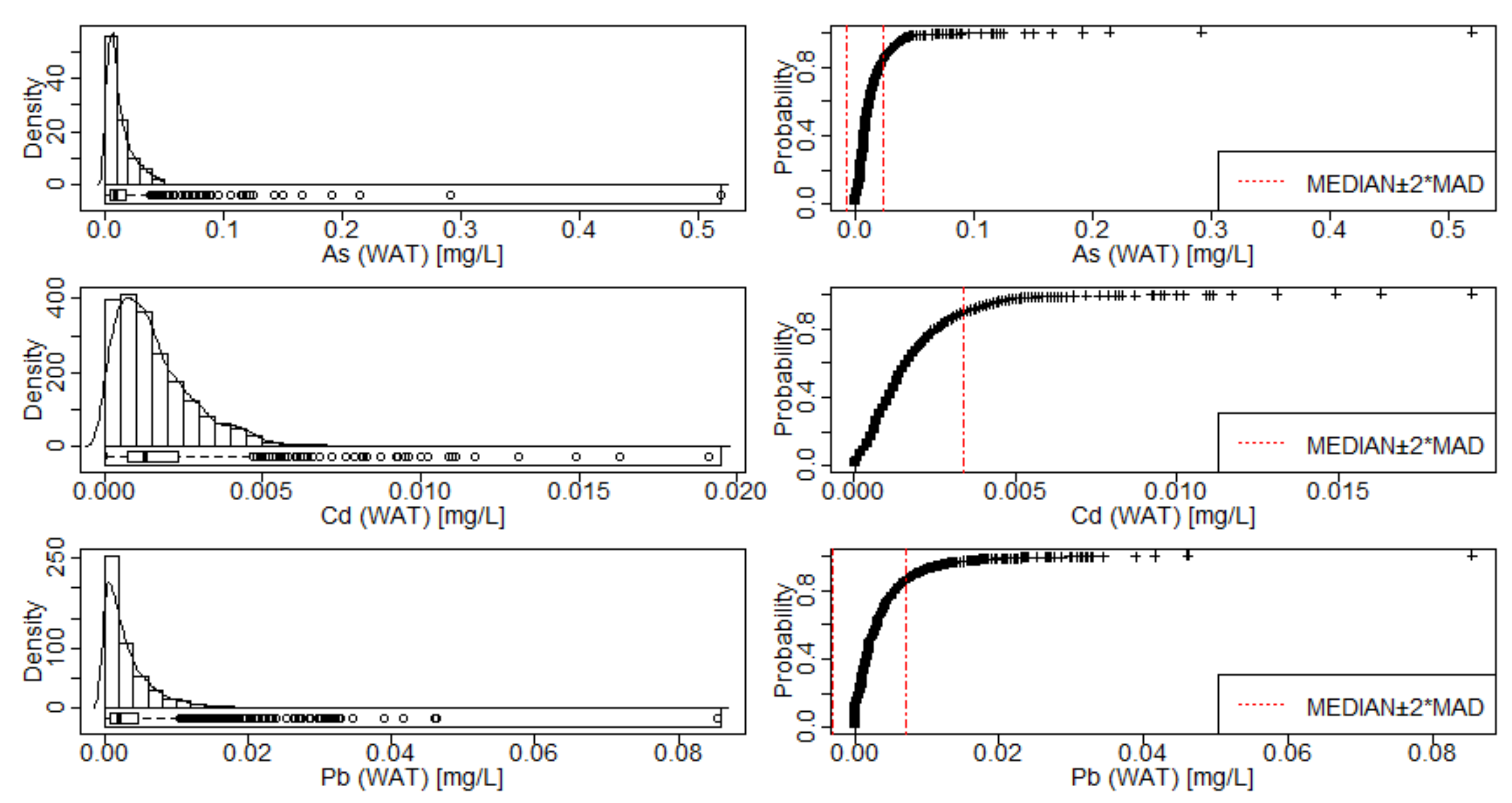
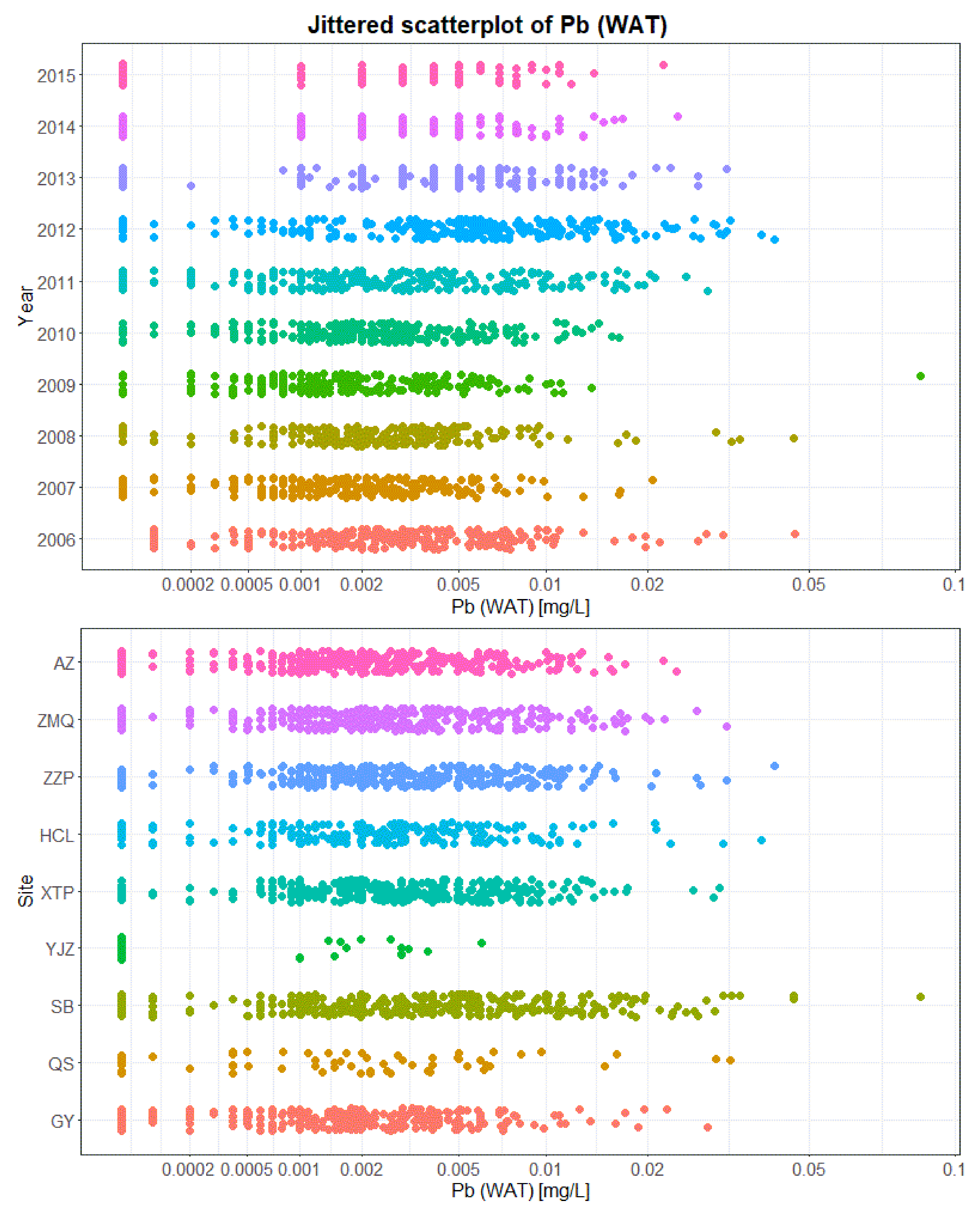
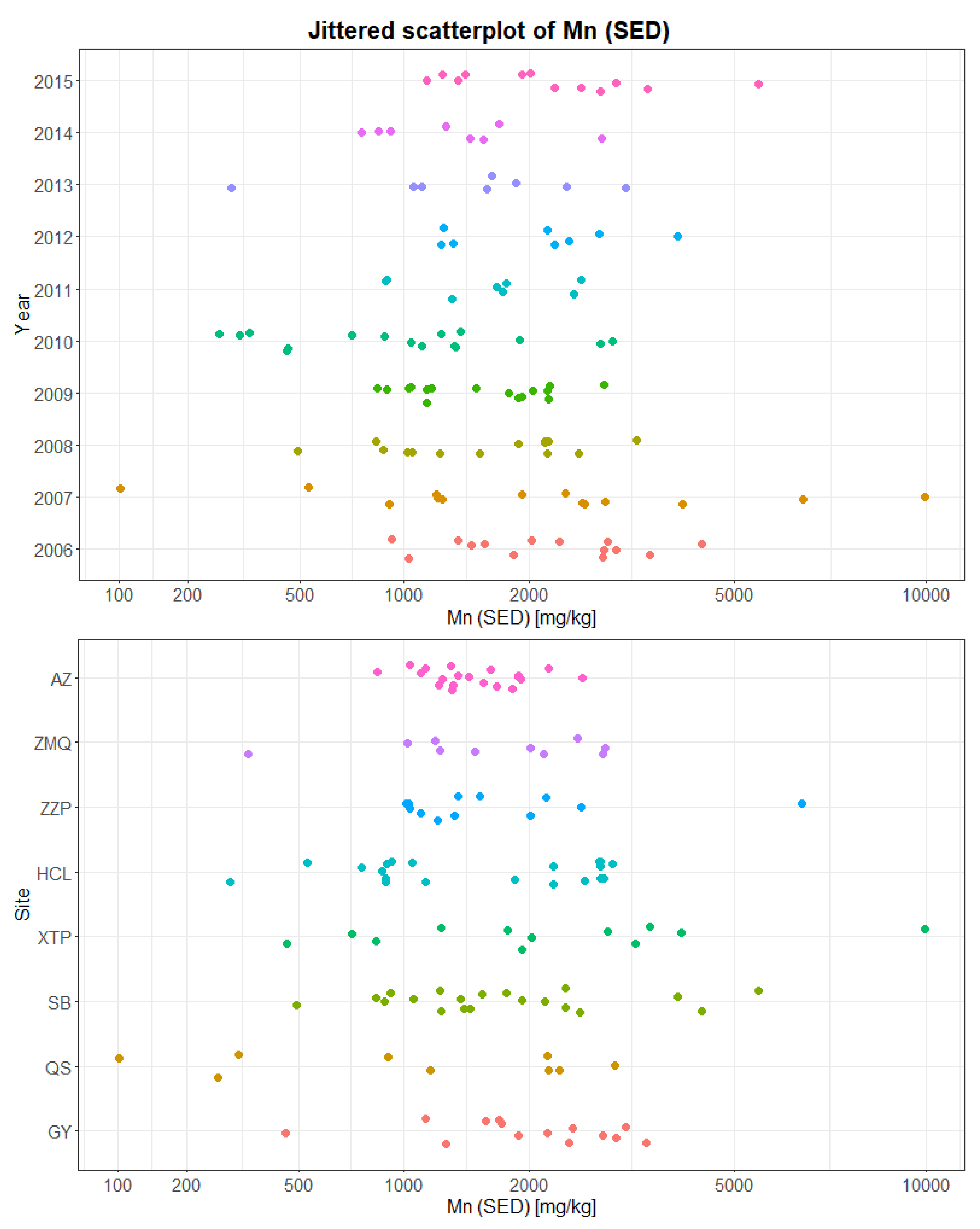
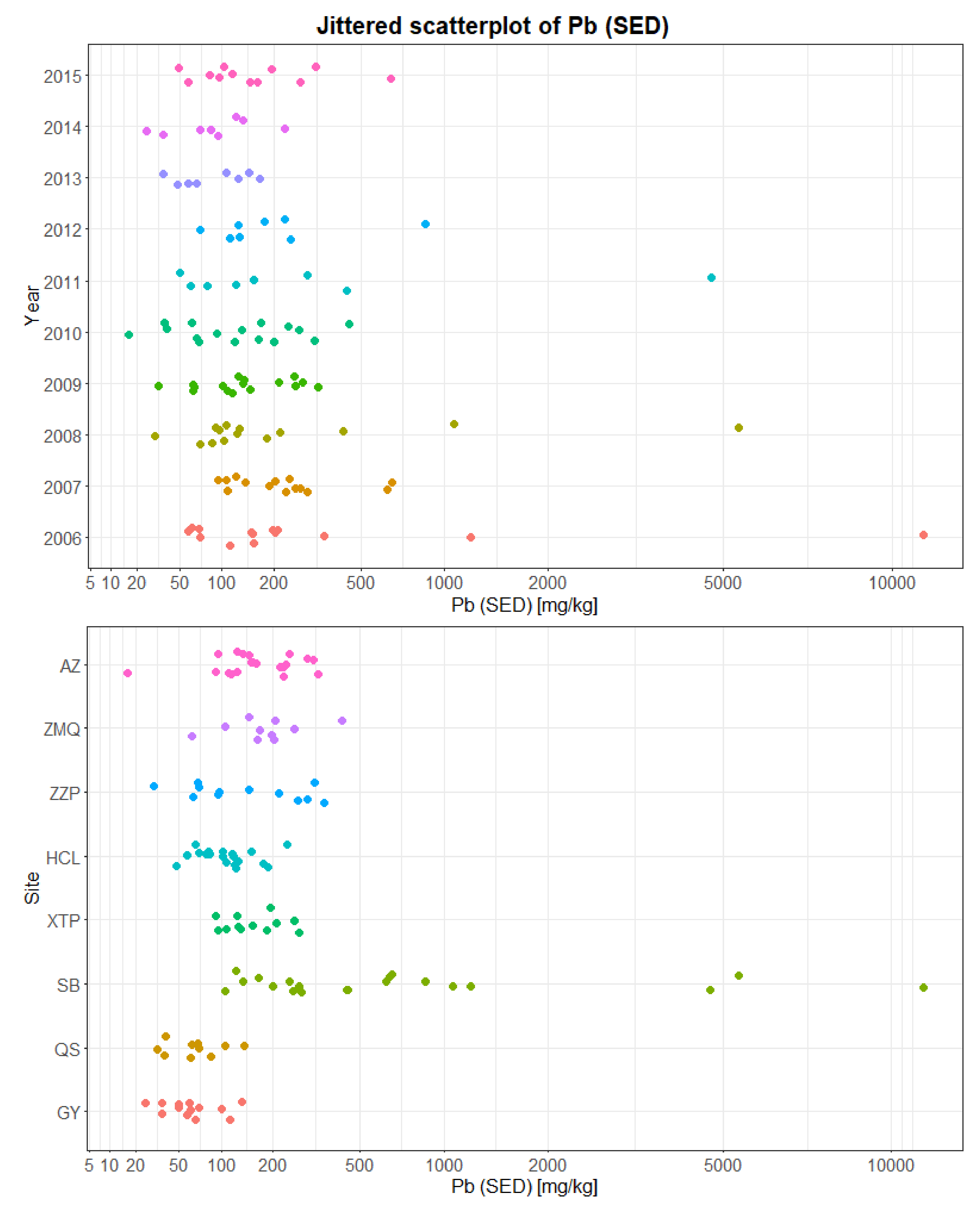
3.1. Sample Visualization and Measures

In the data preparation process, variables that were removed once failed to meet the designated criterion of at least 70% in data validity ratio (after which, the variables that remained in the WAT were As, Cd, and Pb; the variables that remained in the SED were Cr, Mn, Cu, Zn, As, Cd, Hg, and Pb).

All variables in WAT and SED, of which each consists of data from all sampling sites in years 2006–2015, were characterized using graphs and statistics. Combined plots of histogram, boxplot, and density trace (left) and ECDF-plots (right) for variables in WAT and SED were shown in Figure 2 and Figure 3, respectively, with the ranges of [MEDIAN ± 2 × MAD] marked in each ECDF-plot as a visual indicator for the range in which the main part of data was concentrated. A summary of the statistics was shown in

Table 1. Summary table of studied heavy metal variables.

Variable	MIN	MEDIAN	MEAN	MAX	MAD	SD	IQR	CV%	CVR%	G1	G1*
As (WAT)	0.000035	0.00876	0.01358	0.52	0.007798	0.01881	0.009859	138.53	89.02	11.12	5.76
Cd (WAT)	0.00005	0.0013	0.001674	0.0191	0.001038	0.001532	0.001186	91.51	79.83	2.96	2.59
Pb (WAT)	0.00005	0.0020	0.003617	0.0854	0.00252	0.004957	0.002817	137.06	126.02	4.52	3.30
Cr (SED)	11.7	54.80	54.59	131	14.35	20.54	15.02	37.63	26.19	0.31	−0.06
Mn (SED)	101	1620	1884	9950	873.3	1275	954.4	67.68	53.90	2.83	1.39
Cu (SED)	15.4	62.85	112.1	1650	39.88	201.4	45.39	179.69	63.46	5.67	5.38
Zn (SED)	63.0	418.5	659.7	11,900	229.8	1343	235.6	203.58	54.91	6.60	6.34
As (SED)	16.3	62.95	135.2	1561	49.15	246.2	69.97	182.06	78.07	4.34	4.58
Cd (SED)	0.086	8.595	21.66	829	8.903	78.90	8.766	364.29	103.58	9.45	5.17
Hg (SED)	0.011	0.2505	1.192	52.63	0.1683	5.726	0.2174	480.27	67.18	7.48	7.41
Pb (SED)	16.1	128.5	359.4	11,200	94.44	1203	107.7	334.61	73.50	7.41	6.76

MIN = minimum value; MAX = maximum value; SD = standard deviation; MAD = median absolute deviation standardized to conform to the normal distribution; IQR = interquartile range standardized to conform to the normal distribution; CV = coefficient of variation (per cent); CVR = robust coefficient of variation (per cent); G₁ = sample skewness; G₁* = sample skewness with the maximum value removed. n = 2553 for WAT and n = 118 for SED, no missing values. All values in WAT are in mg/L, and all values in SED are in mg/kg.

. There were 2553 samples in the WAT and 118 in the SED.

Various extents of positive skewness were observed from all studied variables in WAT and SED. The As (WAT) displayed the most prominent positive skewness in all studied variables, with the maximum value being more than 50 times of IQR above the median and the sample skewness being the highest 11.12. The Cr (SED) had the lowest sample skewness value of 0.31, of which the sample distribution shape was approximately symmetrical. Cd (WAT), Mn (SED), and As (SED) possessed comparatively moderate skewness levels, and the rest of the variables had relatively strong skewness levels. The extent of skewness was also observed by the inflation of MEAN, SD, and CV against MEDIAN, MAD, and CVR, respectively.

From the graphs, it was observed that a single value was significantly departed from other values in As (WAT), Pb (WAT), and Cd (SED). Some of the statistics were severely inflated by this single value. To reveal the potential influence on skewness from the maximum value, the coefficient of skewness was again calculated but removing the maximum value from each variable, and the results were shown in Table 1 as G₁*. The sample skewness of As (WAT) greatly dropped from 11.12 to 5.76 when the maximum value was removed. Cr (SED) had a negative G₁* and was very close to zero. The skewness of other variables was decreased to a certain extent.

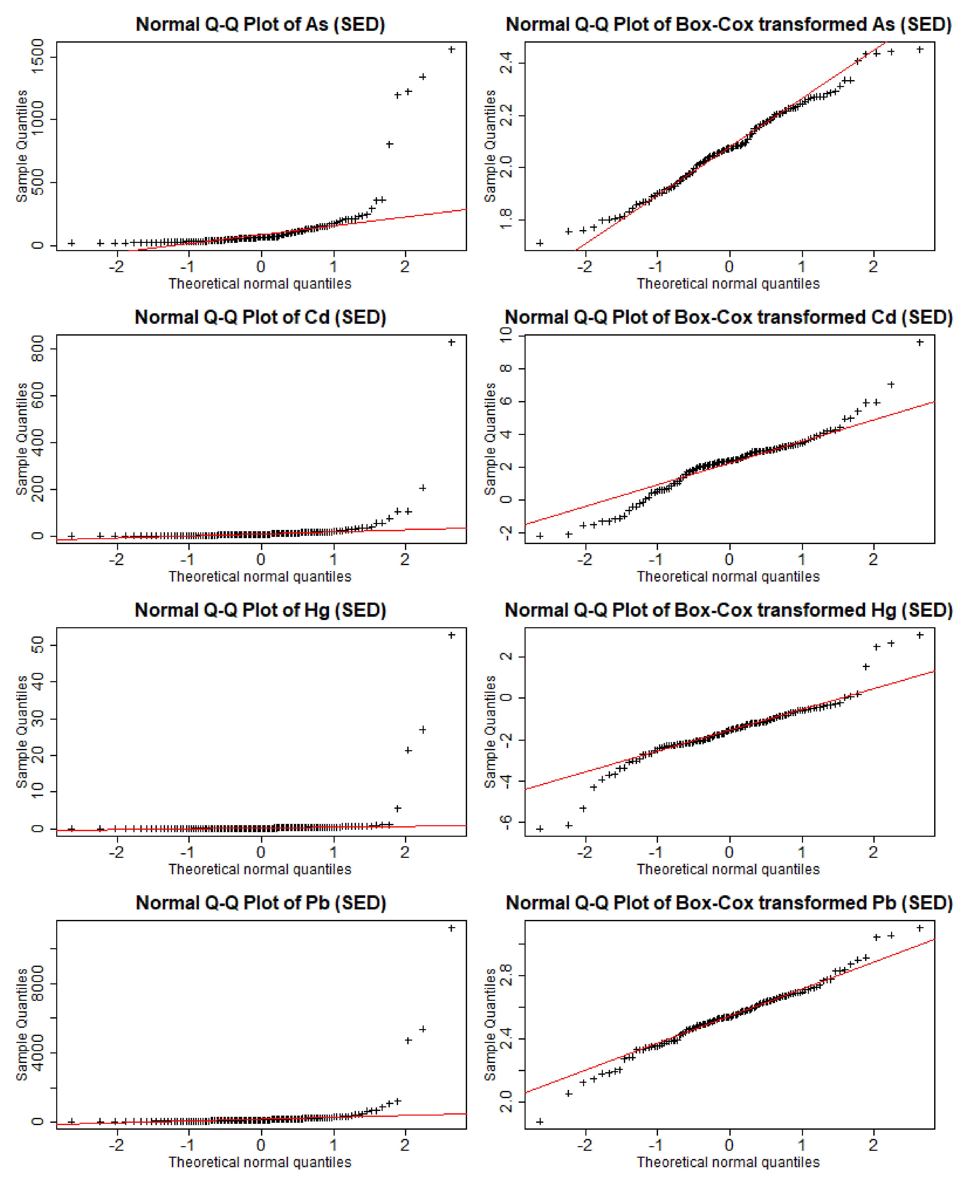
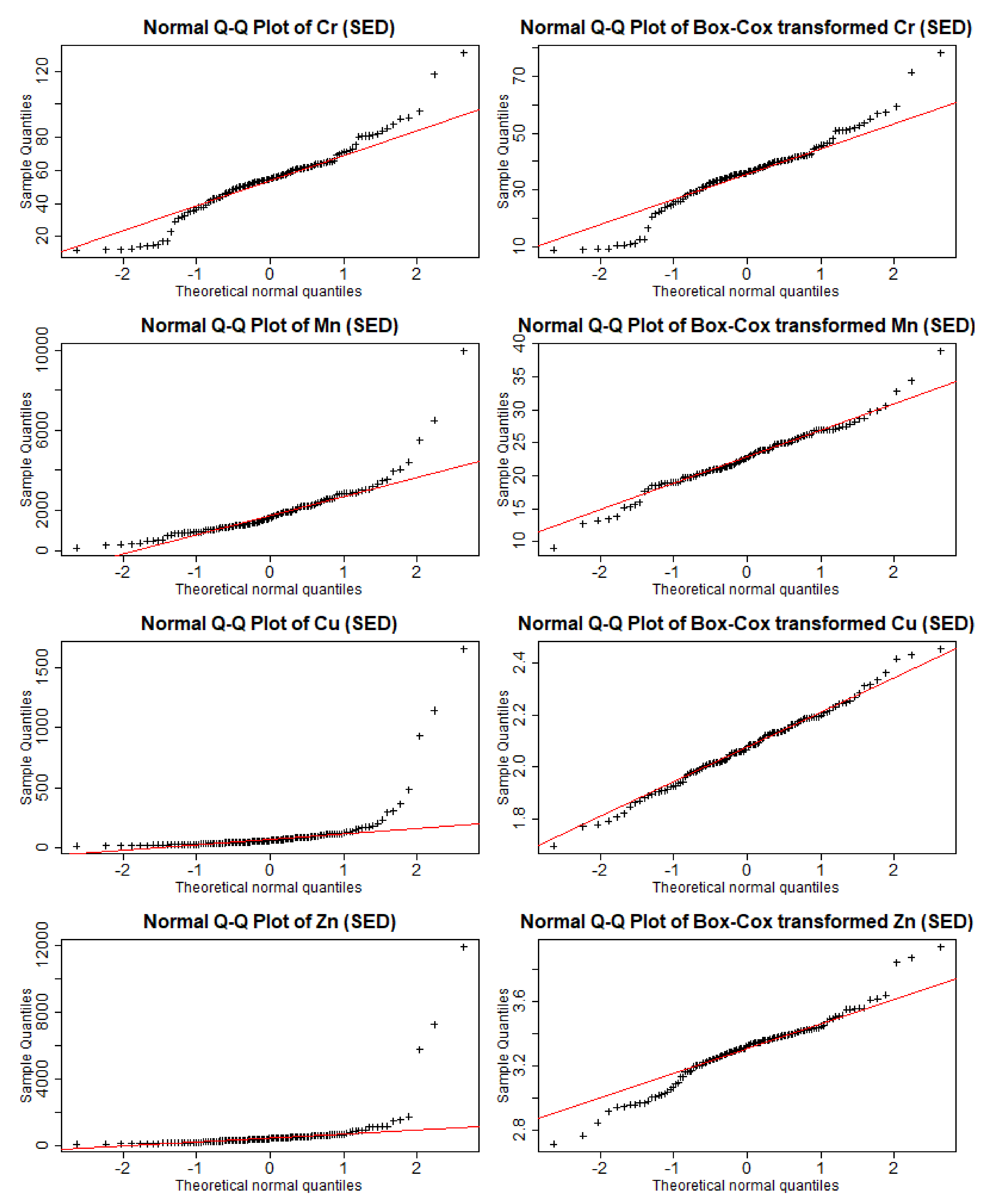
3.2. Transformation and Normality Test

Histogram, boxplot, density trace, and ECDF-plot of variables in WAT and SED after Box-Cox transformation were in Figure 4 and Figure 5. The lambda (λ) values of the transformations were marked on each ECDF-plot. The values corresponding to both the lower detection limits (DL transformed) and half of the lower detection limits (DL/2 transformed) were marked in the ECDF-plots in Figure 4. The normal Q-Q plots of raw and Box-Cox transformed variables in WAT and SED were given in Appendix B.

The λ value for Cr (SED) was close to 1, indicating a roughly linear transformation. The λ values for Cd (SED) and Hg (SED) were approximately zero, for which a log-transformation could also suffice.

p-values (α = 0.01) of S-W normality test on the raw and Box-Cox transformed variables in WAT and SED were in

Table 2. Shapiro-Wilk test p-values for raw and Box-Cox transformed variables.

Variable	Raw	Box-Cox
As(WAT)	4.11 × 10−65 ***	4.34 × 10−24 ***
Cd(WAT)	6.04 × 10−50 ***	2.38 × 10−13 ***
Pb(WAT)	1.13 × 10−58 ***	1.12 × 10−25 ***
Cr(SED)	7.66 × 10−4 ***	9.42 × 10−4 ***
Mn(SED)	9.80 × 10−12 ***	4.23 × 10−2 *
Cu(SED)	2.91 × 10−20 ***	9.21 × 10−1
Zn(SED)	3.48 × 10−21 ***	5.33 × 10−3 **
As(SED)	1.68 × 10−19 ***	3.74 × 10−1
Cd(SED)	1.56 × 10−22 ***	2.30 × 10−4 ***
Hg(SED)	7.81 × 10−23 ***	1.71 × 10−6 ***
Pb(SED)	3.15 × 10−22 ***	1.05 × 10−1

* p < 0.05; ** p < 0.01; *** p < 0.001.

. The p-values of raw variables were all below the significance level of 0.01, which indicate a significant deviation from the normal distribution in the samples. Box-Cox-transformed Cu, Zn, As, and Pb in SED had p-values above the significance level of 0.01, which gave little evidence of departure from normality, and led to the acceptance of normality in these Box-Cox-transformed variables. Limited improvement in normality was found for Cr (SED), whereas good improvements in normality were observed for all other variables.

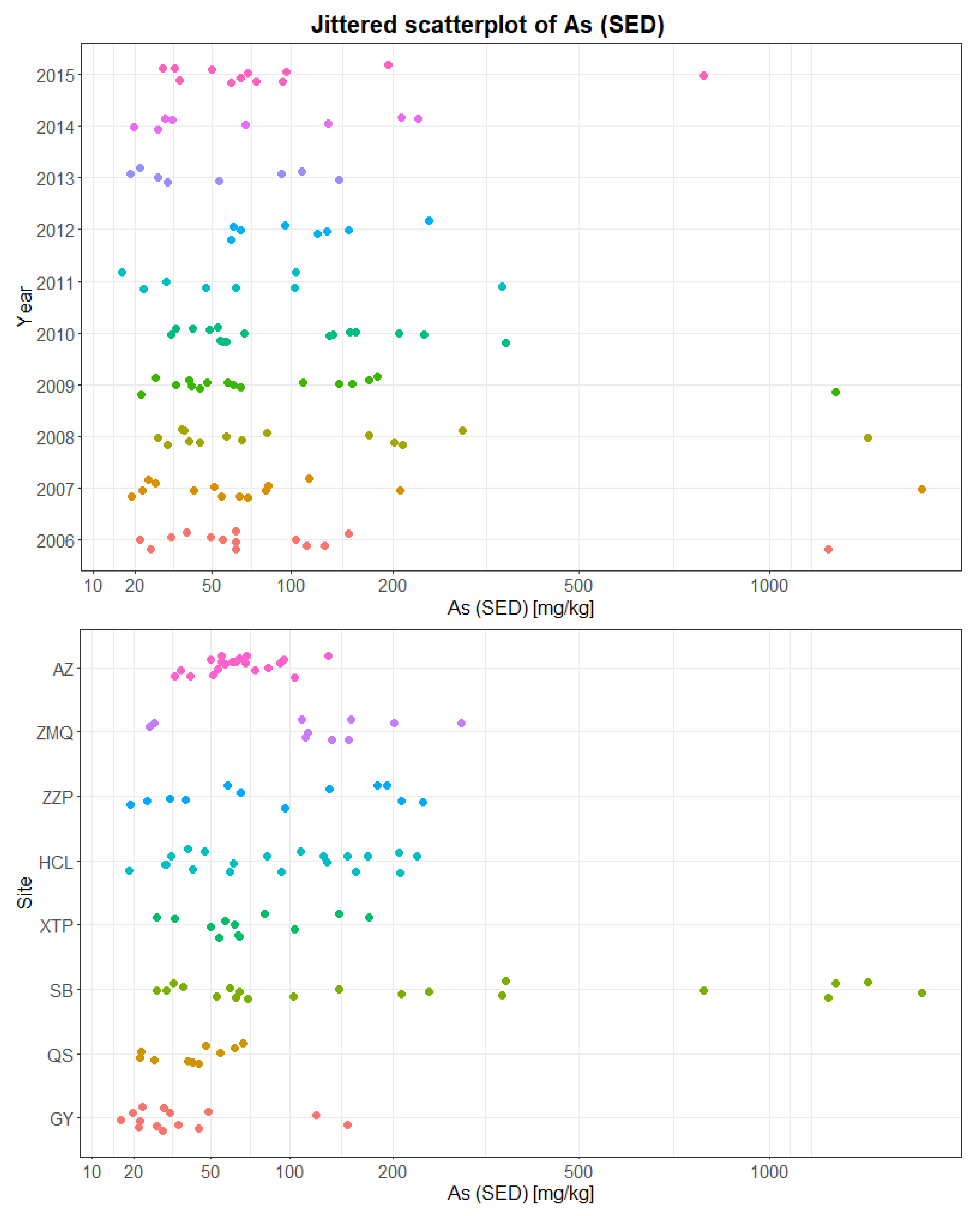
3.3. Characterizing Temporal and Spatial Dependency

The studied variables were based on data with various time and space origins, which were presumably inhomogeneous. The factors of time and space were used as indexes for subdividing subsets in this study. Scatterplots of all variables were drawn with samples grouped by either year or sampling site and were horizontally scaled by Box-Cox transformation (Appendix C).

4. Discussion

4.1. The Sample Distributions of Heavy Metal Variables

It has been widely observed in environmental and geochemical studies that the sample distribution of an environmental substance is positively skewed (and may have a roughly log-normal shape), which is resulted from combined processes, including mixed geochemical processes, industrial pollution, and human interference [7,22,23]. The data used in the present study covers large longitude in both time and distance that the influences from multiple processes, i.e., positive skewness should be expected. The time-and-space aggregated samples of As, Cd, Pb in WAT, and Mn, Cu, Zn, As, Cd, Hg, Pb in SED, showed prominent positive skewness in the distribution shapes. However, Cr (SED) stood out with a roughly bell-shaped sample distribution, with two major gaps at ~10 and ~90 percentile. Mn (SED) presented slightly heavier positive skewness than Cr (SED) but still possessed a much weaker skewness than other variables. The main body of Mn (SED) was symmetrical, and the skewness was mainly induced by six positively deviated values.

After the Box-Cox transformation, the influence of data censoring on the sample distribution became visible in the WAT data set, while the SED data set has no censored values. These censored values were presented on ECDF curves as stacked bars, which were marked in Figure 4. In normal Q-Q plots of Box-Cox transformed WAT variables (Appendix B), the censored values (long horizontal bars) were the most prominent factor that deviated the curves from linear trends, which could explain that all Box-Cox transformed WAT variables failed the S-W normality test.

The values that correspond to DL/2 were introduced in the data preparation process, in which all censored values were set to half of the DLs. The values that were equal to or less than the DLs were most likely from the data in the year 2006, in which the original report failed to distinguish censored data. These data in 2006 were treated as valid values due to the absence of specification in the original reports. As a special case, the DL of As (WAT) had changed from 0.007 mg/L to 0.00007 mg/L since April 2010. In Figure 4, three discrete vertical bars that were stacked on the ECDF curve of the As (WAT) correspond to the transformed values of the improved DL/2 (0.000035 mg/L), the former DL/2 (0.0035 mg/L), and the former DL (0.007 mg/L), respectively.

In addition, the WAT data set had discretization in the sample distribution, which was due to limitations in analytical precision and rounding of relatively small values.

4.2. The Temporal and Spatial Characteristics

The relevance of the WAT variables with factors of time and space was addressed (Figure A4, Figure A5 and Figure A6).

The levels of As (WAT) and Cd (WAT) presented a decreasing trend over the studied period. Some positively deviated values were observed in 2006–2009 in As (WAT) and in 2006–2010 in Cd (WAT), but no deviated values in the corresponding ranges could be seen in the following studied time period. Besides, a lowering trend on the concentration of values was visually recognized in these two variables. The Pb (WAT) had a distinctive temporal behavior that the proportion of censored values per each year dramatically increased from 5.8% (2011), 6.1% (2012), to 14.4% (2013), and finally to 47.2% (2014) and 52.1% (2015). This can be considered as a sign of a decreasing trend in its values, although the main body of the samples slightly spread out to higher contamination levels in 2011–2013. Statistical evidence to support the decreasing trends in As, Cd, and Pb in WAT was given by performing one-sided hypothesis tests for a difference between two means for every two consecutive years per each element. The hypotheses of this series of tests can be generalized as:

• H₀: there is no difference between the means of two consecutive years.
• H_a: the mean of the year is significantly larger than the mean of the next year.

Conditions were checked, and the t-procedure does apply. The resulting p-values of t-tests were present in

Table 3. p-values of one-sided hypothesis tests for the difference between two consecutive years.

Variable	2006–2007	2007–2008	2008–2009	2009–2010	2010–2011	2011–2012	2012–2013	2013–2014	2014–2015
As(WAT)	2.21 × 10−1	9.97 × 10−1	1.16 × 10−5 ***	1.85 × 10−3 **	8.93 × 10−1	1.98 × 10−7 ***	2.02 × 10−6 ***	4.82 × 10−1	9.71 × 10−1
Cd(WAT)	6.22 × 10−10 ***	5.97 × 10−1	6.42 × 10−1	8.68 × 10−1	9.64 × 10−1	3.54 × 10−2 *	1.21 × 10−7 ***	1.54 × 10−20 ***	3.18 × 10−9 ***
Pb(WAT)	4.75 × 10−8 ***	9.99 × 10−1	5.74 × 10−2	9.11 × 10−1	9.97 × 10−1	1.00 × 100	6.20 × 10−7 ***	1.11 × 10−12 ***	2.89 × 10−1

* p < 0.05; ** p < 0.01; *** p < 0.001.

. It should be noted that the significant (p < 0.01) decrease in sample means of As (WAT) from 2009 to 2010 could be dominated by the lowering of its DL, as discussed in Section 4.1.

Judging from Figure A4, Figure A5 and Figure A6 and Table 3, a conclusion was drawn that significant (p < 0.001) decreasing trends in the contamination level of As, Cd, and Pb in WAT did occur, starting from 2012, 2013, and 2013, respectively. This characteristic coincided in time with a series of environmental protection actions conducted by the government to control pollutions in the fluvial environment of Xiangjiang River, which was provoked in 2011 and initiated soon afterward [24]. In detail, a collection of policies was approved by the State Council of China, namely the “12th Five-Year Plan on Prevention and Control of Heavy Metal Pollution” and “Xiangjiang River Basin Control Plan for Heavy Metal Pollution” [5,25,26]. As one of the goals in implementing the control and treatment plan on heavy metals in Xiangjiang Basin, discharges from industries with heavy metal pollution were designated to cut off by 50% in the whole watershed by the end of its 5-year period, compared to 2008. The water monitoring data presented clear evidence of benefits from these environmental policies.

For the space factor, Songbai (SB) was noticeably the most heavily contaminated site for all three elements in WAT, indicating major discharges of pollutants at this location. Less positively deviated values were seen at monitoring stations downstream of SB, such as at Xintangpu (XTP) and Huangchaling (HCL). At Zaoziping (ZZP), the contamination levels of As, Cd, and Pb in WAT again increased. At further downstream locations, Zhanmenqian (ZMQ) and Aozhou (AZ), there was a slight decrease in concentration levels.

As for the SED data set (Figure A7, Figure A8, Figure A9, Figure A10, Figure A11, Figure A12, Figure A13 and Figure A14), since (i) it has much less sample size than WAT, and (ii) the samples were only collected in low-water seasons, the SED data set was therefore assumed to contain much less information and variety with regard to the true temporal and spatial characteristics in the studied river segment. The samples of Cr (SED) showed dependence on the time factor, while there was little difference among sites. No clear dependency on either factor was observed in Mn (SED). Relatively space-dependency in Cu (SED), Zn (SED), As (SED), Cd (SED), and Pb (SED) were present that samples from SB distinctively fanned out towards high concentrations, and the upper stream sites GY and QS had comparatively low concentration values. Hg (SED) had slightly both temporal and spatial dependency, which displayed similar spatial patterns with other five SED variables but also had lower concentration levels in 2013 and higher levels in 2006 and 2007.

Besides, slightly decreasing trends were observed in SED commencing in 2012, where the above-discussed control and treatment plan in Xiangjiang Basin took place. Due to the loss of variability information in SED, this could only serve as a clue that alleviation of pollutants in the water column may have a positive relationship with that in the sediment, but the effects are slow and much less significant.

The major sources of pollutants in water and sediment were identified to be close to sites of SB and ZZP, where concentration levels abruptly increased. SB has intensive smelting and manufacturing industries, while ZZP is located downstream of Hengyang City, which could explain the source of the elevated concentrations. The confluence with river branches directly at downstream of SB, ZZP, and ZMQ may have the effect of diluting the concentrations of each element. The effects of dilution and dispersion could explain the lower number of deviated values at sites downstream of SB, as well as the slight decrease in concentration levels after ZZP and ZMQ.

4.3. The Unique Behavior of Cr

From Figure A7, it was observed that the ranges of Cr (SED) could have substantial variation between years, which was greater in its extent when compared with other studied SED variables. Generally, the values of Cr (SED) fell in 30–100 mg/kg. While in 2010, the sample values were in 10–30 mg/kg, which was exceptionally low. Besides, in 2007–2009, the sample values were narrowly clustered, while in many other years, the sample distributions were relatively spread out. In addition, the above discussed environmental policies initiated in 2011 coincided with a visible decreasing trend in Cr (SED) starting from 2012. Considering the small difference among spatial groups, these above observations may indicate a relatively fast process of deposition-releasing equilibrium of Cr between water column and sediment, which gave sedimentary Cr the mobility to present greater potentials of variability in its time-series than other variables studied. Despite our best efforts, we failed to solidify this explanation with literature, but we did present it as a hypothetical characteristic.

4.4. Implications for Further Data Analyses

Normality is a most common assumption in many statistical procedures applied in environmental studies, such as ANOVA and factor analysis (FA). Even in principal component analysis (PCA) where normality is not a basic assumption, this procedure is still sensitive to non-normality [12]. Entering these processes with highly skewed data could violate the assumption and/or lead to biased and unstable results.

This study showed that data censoring and too severe rounding were the two prominent factors in WAT that led to non-normality after Box-Cox transformation. The inhomogeneity in WAT and SED may drive procedures such as PCA, FA, and regression analysis to discriminate the difference among subgroups rather than fulfilling their initial task of disclosing internal structures and patterns in the data. For the potentially inhomogeneous variables in SED, the best way to achieve better exploratory analyzing results would be subdividing the data into homogeneous groups.

5. Conclusions

In the present study, the sample distributions of three heavy metal elements in water and eight in surface sediment in Hengyang segment, Xiangjiang River were analyzed based on the 10-year environmental monitoring data sets. We discovered that:

• The heavy metal elements of As, Cd, and Pb in water column and Mn, Cu, Zn, As, Cd, Hg, and Pb in sediment that consisted of all available data covered in this study were generally positively skewed in distribution shape. However, the Cr in sediment presented roughly symmetrical sample distribution shape. The unique behavior of Cr in sediment was discussed, and a possible explanation was given that a relatively fast process of deposition-releasing equilibrium of Cr between water column and sediment was present.
• Box-Cox transformation has effectively improved the normality of all variables; however, data censoring and the discretization in samples have a negative effect on its outcome.
• The large sample size in the water monitoring data set avails a better discovery of the temporal and spatial characteristics in the data, such that the influence of policy interference and river branches were discovered. The sediment data set contained much less temporal and spatial information, but the dependence on space was more visible than the dependence on time for most of the studied elements (except in the case of Cr, which only showed clear relations with the time factor).

References

1. Karageorgis, A.P.; Sioulas, A.; Krasakopoulou, E.; Anagnostou, C.L.; Hatiris, G.A.; Kyriakidou, H.; Vasilopoulos, K. Geochemistry of surface sediments and heavy metal contamination assessment: Messolonghi lagoon complex, Greece. Environ. Earth Sci. 2012, 65, 1619–1629. [Google Scholar] [CrossRef]
2. Hudson-Edwards, K.A. Sources, mineralogy, chemistry and fate of heavy metal-bearing particles in mining-affected river systems. Mineral. Mag. 2003, 67, 205–217. [Google Scholar] [CrossRef]
3. Li, F.; Zhang, J.; Jiang, W.; Liu, C.; Zhang, Z.; Zhang, C.; Zeng, G. Spatial health risk assessment and hierarchical risk management for mercury in soils from a typical contaminated site, China. Environ. Geochem. Health 2017, 39, 923–934. [Google Scholar] [CrossRef] [PubMed]
4. Yang, Z.; Wu, Z.; Liao, Y.; Liao, Q.; Yang, W.; Chai, L. Combination of microbial oxidation and biogenic schwertmannite immobilization: A potential remediation for highly arsenic-contaminated soil. Chemosphere 2017, 181, 1–8. [Google Scholar] [CrossRef] [PubMed]
5. Hu, H.; Jin, Q.; Kavan, P. A study of heavy metal pollution in China: Current status, pollution-control policies and countermeasures. Sustainability 2014, 6, 5820–5838. [Google Scholar] [CrossRef]
6. Zitko, V. Principal component analysis in the evaluation of environmental data. Mar. Pollut. Bull. 1994, 28, 718–722. [Google Scholar] [CrossRef]
7. Loska, K.; Wiechuła, D. Application of principal component analysis for the estimation of source of heavy metal contamination in surface sediments from the Rybnik Reservoir. Chemosphere 2003, 51, 723–733. [Google Scholar] [CrossRef]
8. Simeonov, V.; Massart, D.; Andreev, G.; Tsakovski, S. Assessment of metal pollution based on multivariate statistical modeling of “hot spot” sediments from the Black Sea. Chemosphere 2000, 41, 1411–1417. [Google Scholar] [CrossRef]
9. Tam, N.F.Y.; Wong, Y.-S. Spatial variation of heavy metals in surface sediments of Hong Kong mangrove swamps. Environ. Pollut. 2000, 110, 195–205. [Google Scholar] [CrossRef]
10. Mao, L.; Mo, D.; Guo, Y.; Fu, Q.; Yang, J.; Jia, Y. Multivariate analysis of heavy metals in surface sediments from lower reaches of the Xiangjiang River, southern China. Environ. Earth Sci. 2012, 69, 765–771. [Google Scholar] [CrossRef]
11. Nguyen Van, T.; Ozaki, A.; Nguyen Tho, H.; Nguyen Duc, A.; Thi, Y.T.; Kurosawa, K. Arsenic and heavy metal contamination in soils under different land use in an estuary in northern Vietnam. Int. J. Environ. Res. Public Health 2016, 13, 1091. [Google Scholar] [CrossRef] [PubMed]
12. Reimann, C.; Filzmoser, P.; Garrett, R.; Dutter, R. Statistical Data Analysis Explained: Applied Environmental Statistics with R; John Wiley & Sons: Hoboken, NJ, USA, 2011. [Google Scholar]
13. Hengyang Prefecture, Hunan Province, China. Available online: https://www.mindat.org/loc-713.html (accessed on 29 March 2018).
14. Joanes, D.N.; Gill, C.A. Comparing measures of sample skewness and kurtosis. J. R. Stat. Soc. Ser. D Stat. 1998, 47, 183–189. [Google Scholar] [CrossRef]
15. Box, G.E.; Cox, D.R. An Analysis of Transformations. J. R. Stat. Soc. Ser. B 1964, 26, 211–252. [Google Scholar]
16. Cox, D.R.; Snell, E.J. Analysis of Binary Data; CRC Press: Boca Raton, FL, USA, 1989; Volume 32. [Google Scholar]
17. Shapiro, S.S.; Wilk, M.B. An analysis of variance test for normality (complete samples). Biometrika 1965, 52, 591–611. [Google Scholar] [CrossRef]
18. R Core Team. R: A Language and Environment for Statistical Computing; the R Foundation for Statistical Computing: Vienna, Austria, 2017. [Google Scholar]
19. Filzmoser, P. StatDA: Statistical Analysis for Environmental Data, R package version 1.6.9; 2015. Available online: https://CRAN.R-project.org/package=StatDA (accessed on 29 March 2018).
20. Venables, W.N.; Ripley, B.D. Modern Applied Statistics with S, 4th ed.; Springer: New York, NY, USA, 2002. [Google Scholar]
21. Wickham, H. ggplot2: Elegant Graphics for Data Analysis; Springer: New York, NY, USA, 2009; ISBN 978-0-387-98140-6. [Google Scholar]
22. Chai, L.; Li, H.; Yang, Z.; Min, X.; Liao, Q.; Liu, Y.; Men, S.; Yan, Y.; Xu, J. Heavy metals and metalloids in the surface sediments of the Xiangjiang River, Hunan, China: Distribution, contamination, and ecological risk assessment. Environ. Sci. Pollut. Res. 2017, 24, 874–885. [Google Scholar] [CrossRef] [PubMed]
23. Vistelius, A.B. The skew frequency distributions and the fundamental law of the geochemical processes. J. Geol. 1960, 68, 1–22. [Google Scholar] [CrossRef]
24. Infographic: No.1 Key Project Road Map. Available online: http://www.enghunan.gov.cn/SP/zmxj/ (accessed on 23 March 2018).
25. Jin, S.; Zhou, J.; Yang, F. Government Actions in China’s Green Development. In China Green Development Index Report 2011; Springer: Berlin/Heidelberg, Germany, 2012; pp. 291–316. ISBN 978-3-642-31596-1. [Google Scholar]
26. National “12th Five-Year Plan” for Environmental Protection. Available online: http://english.mep.gov.cn/Resources/Plans/National_Fiveyear_Plan/201606/P020160601356854927248.pdf (accessed on 23 March 2018).
Figure 1. Sampling sites of water and sediment monitoring data. Years of data available for each site are given in the parentheses. The Xiangjiang River flows from south to north.
Sustainability 10 01057 g001
Figure 2. Combined histogram, density trace, and boxplot (left), and empirical cumulative distribution function (ECDF-plot) (right) of As, Cd, and Pb in water monitoring data set (WAT). The ranges of [MEDIAN ± 2 × MAD] are marked in ECDF-plots.
Sustainability 10 01057 g002
Figure 3. Combined histogram, density trace and boxplot (left), and ECDF-plot (right) of Cr, Mn, Cu, Zn, As, Cd, Hg, and Pb in sediment monitoring data set (SED). The ranges of [MEDIAN ± 2 × MAD] are marked in ECDF-plots.
Sustainability 10 01057 g003
Figure 4. Combined histogram, density trace, and boxplot (left), and ECDF-plot (right) of Box-Cox transformed As, Cd, and Pb in WAT. The powers of the transformations are given in the left-side plots, and the transformed values of DL and DL/2 are marked in right-side ECDF-plots.
Sustainability 10 01057 g004
Figure 5. Combined histogram, density trace, and boxplot (left), and ECDF-plot (right) of Box-Cox transformed Cr, Mn, Cu, Zn, As, Cd, Hg, and Pb in SED. The powers of the transformations are given in the left-side plots.
Sustainability 10 01057 g005