First Approach to a Holistic Tool for Assessing RES Investment Feasibility

 , ,
, ,  ,
, 
Abstract
:1. Introduction
2. State-of-the-Art of Energy Estimation Tools
3. Profiling Methodology
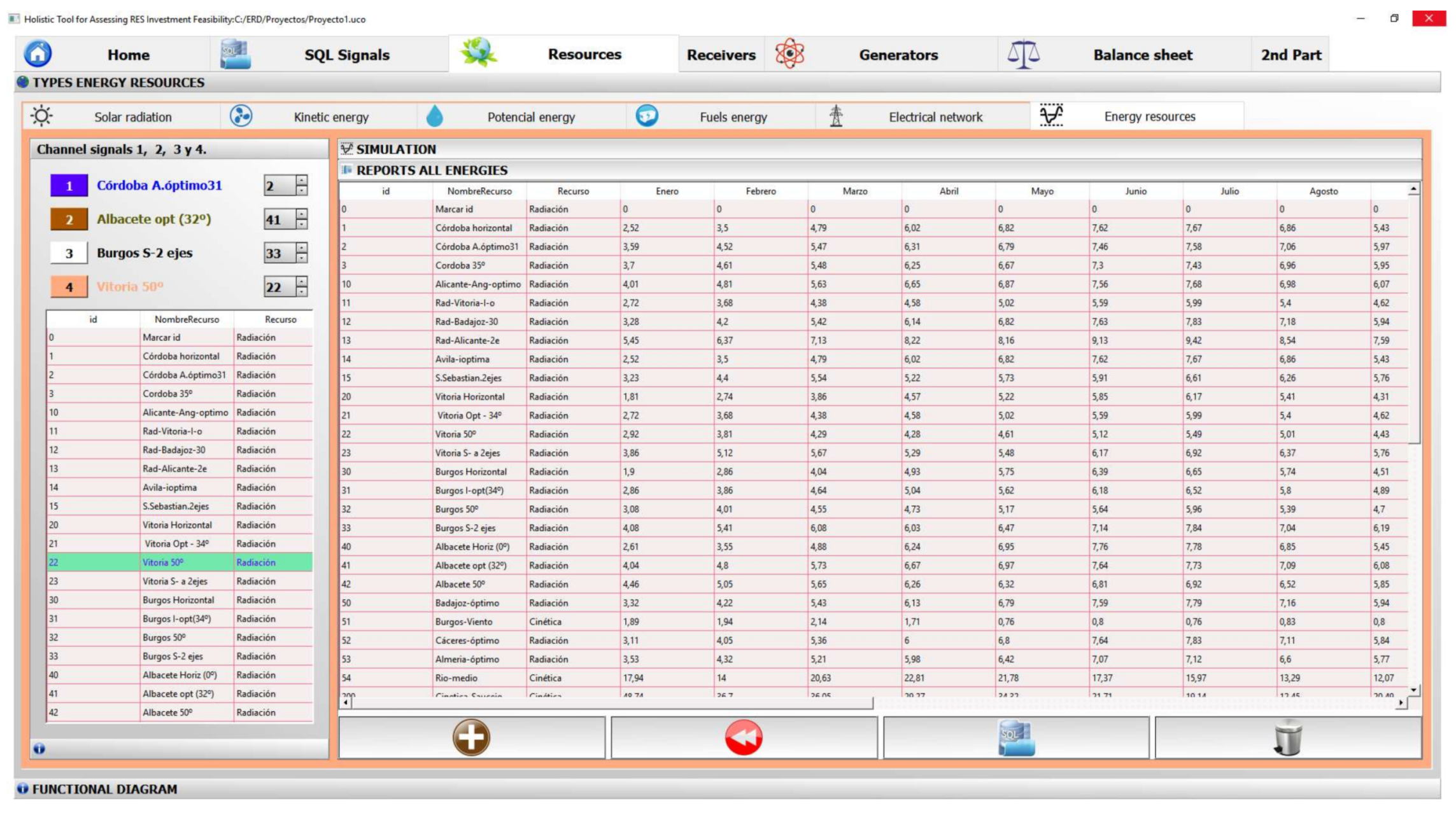
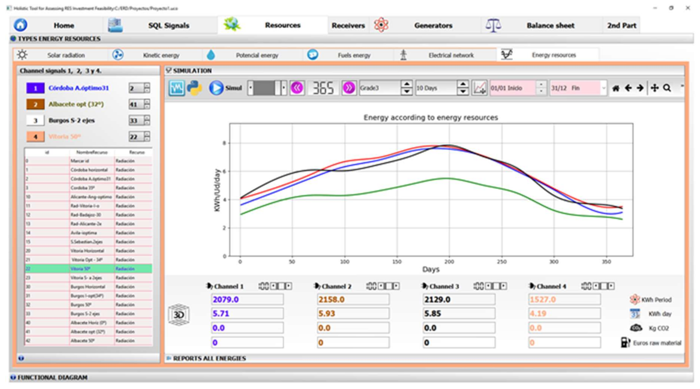
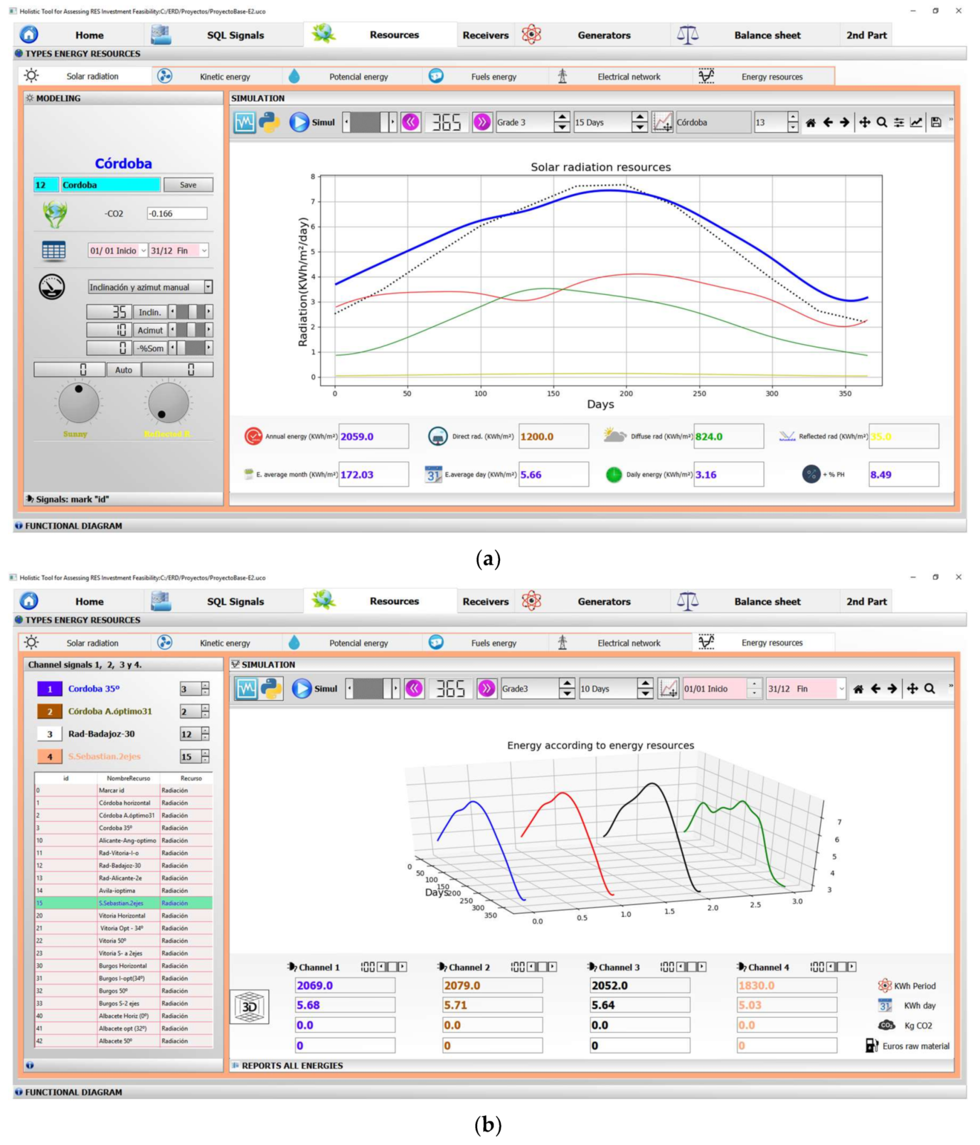
3.1. Profiling Energy Resources
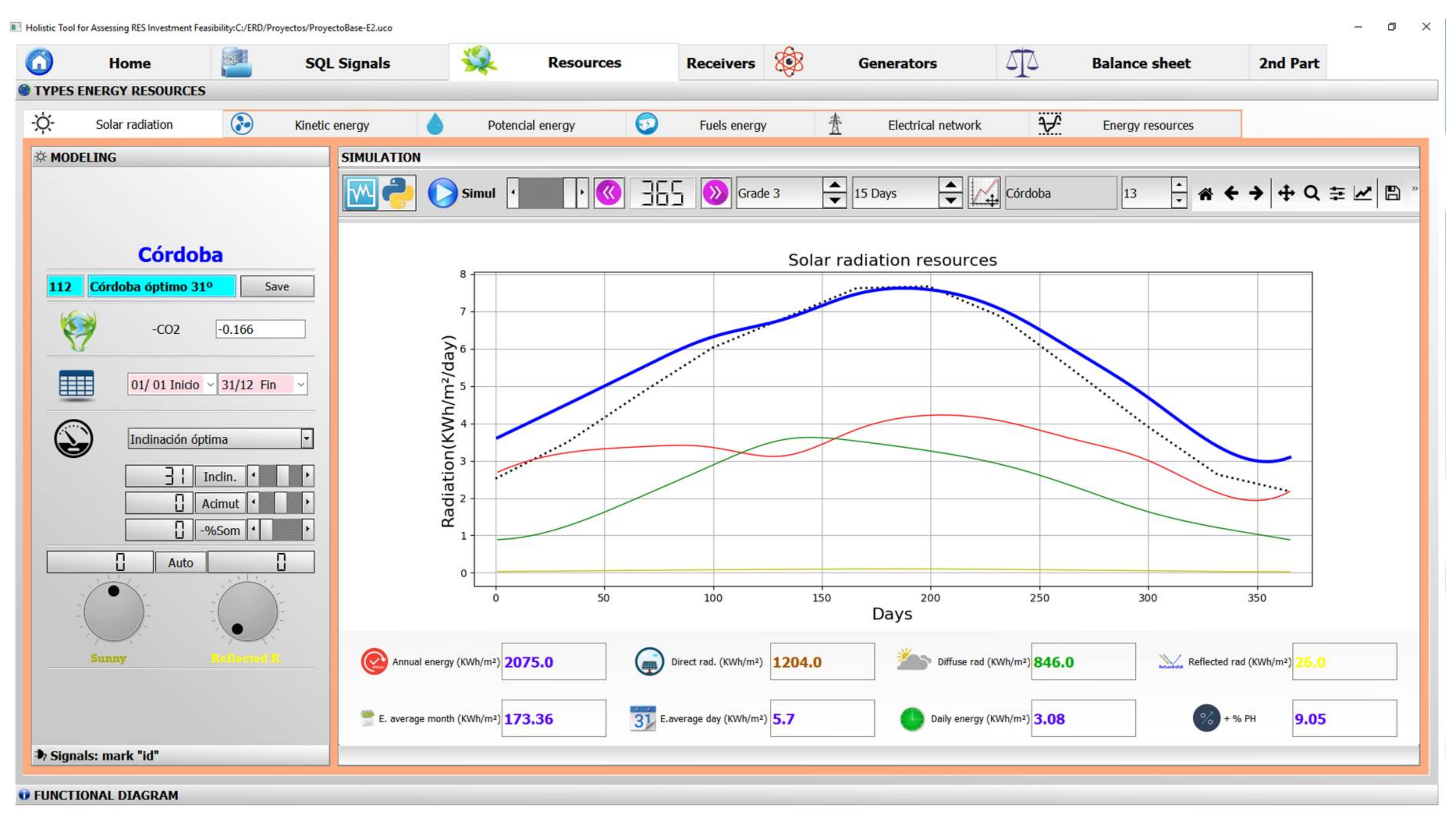
3.1.1. Solar Radiation Estimation and Profiling
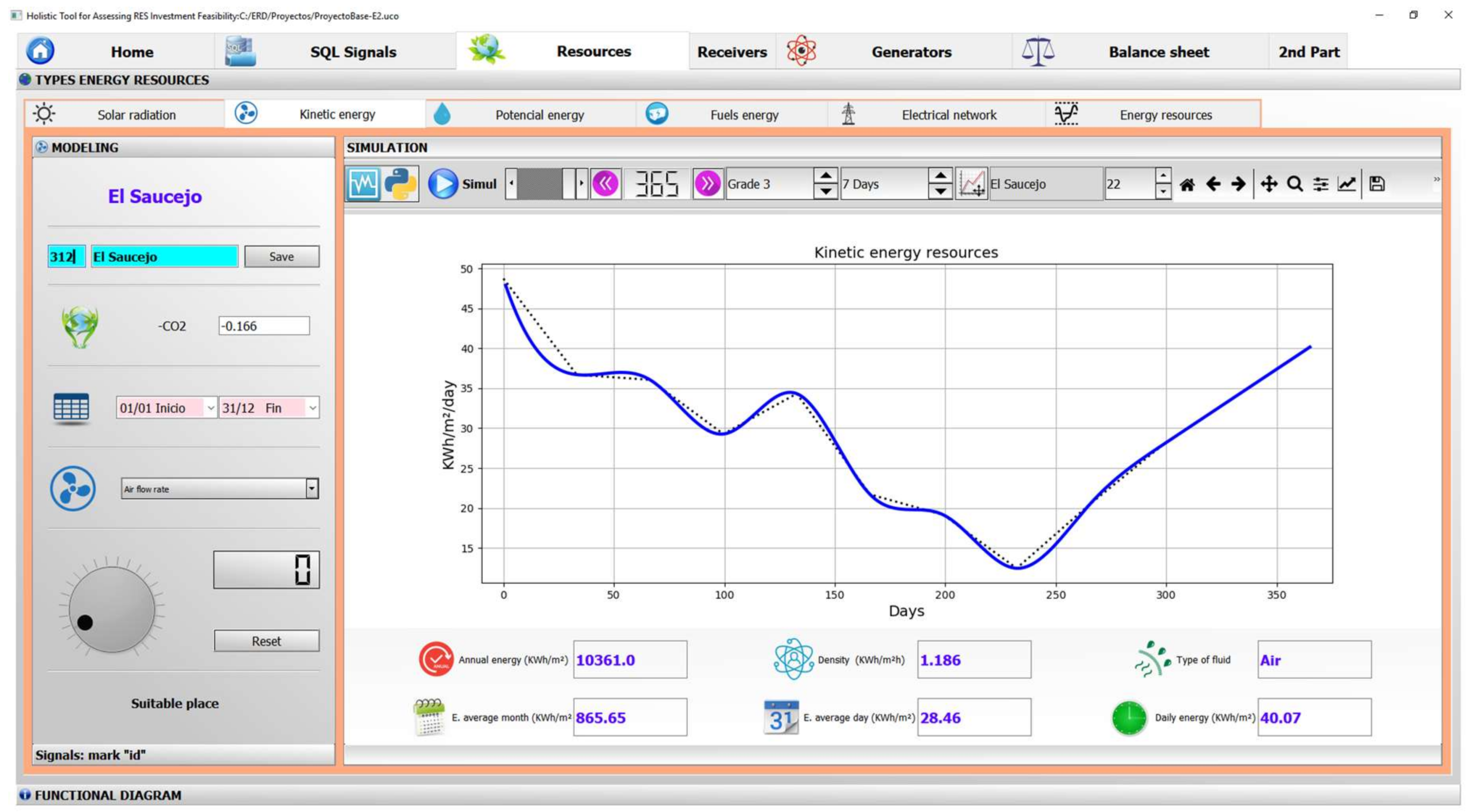
3.1.2. Kinetic Energy Estimation and Profiling
3.1.3. Water Potential Energy Estimation and Profiling Tab
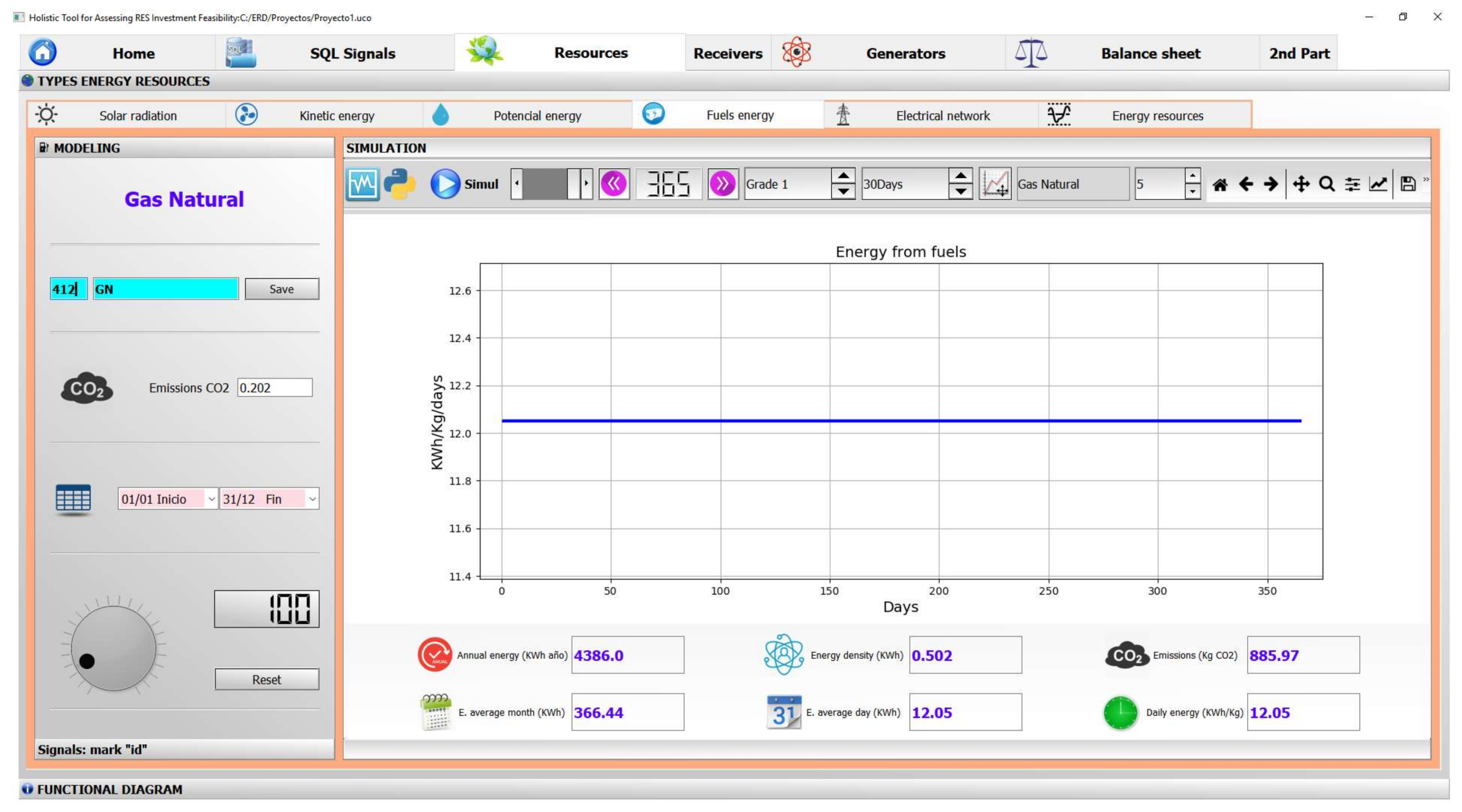
3.1.4. Fuel Energy Estimation and Modeling, Additional Data and Comparison Features Tab
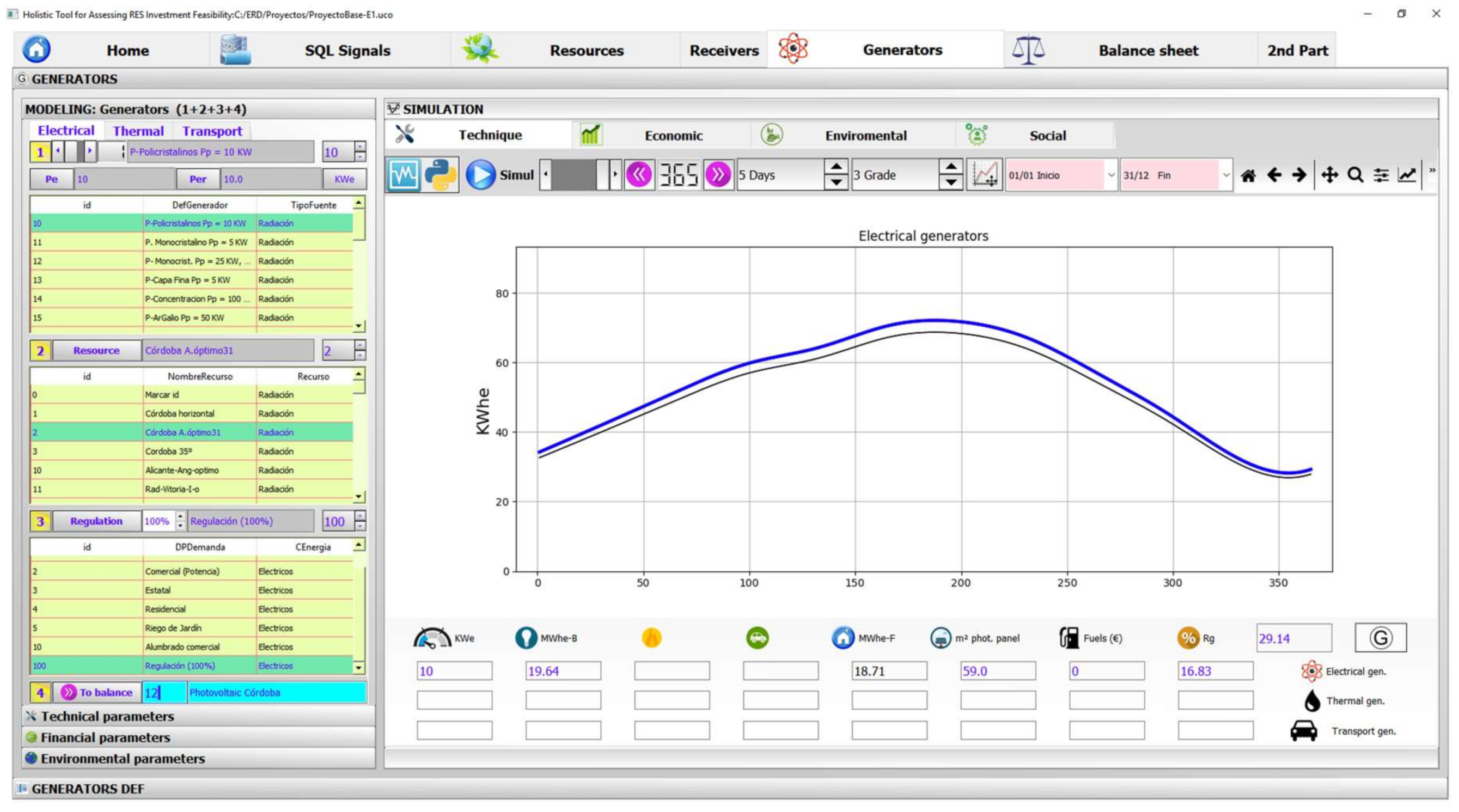
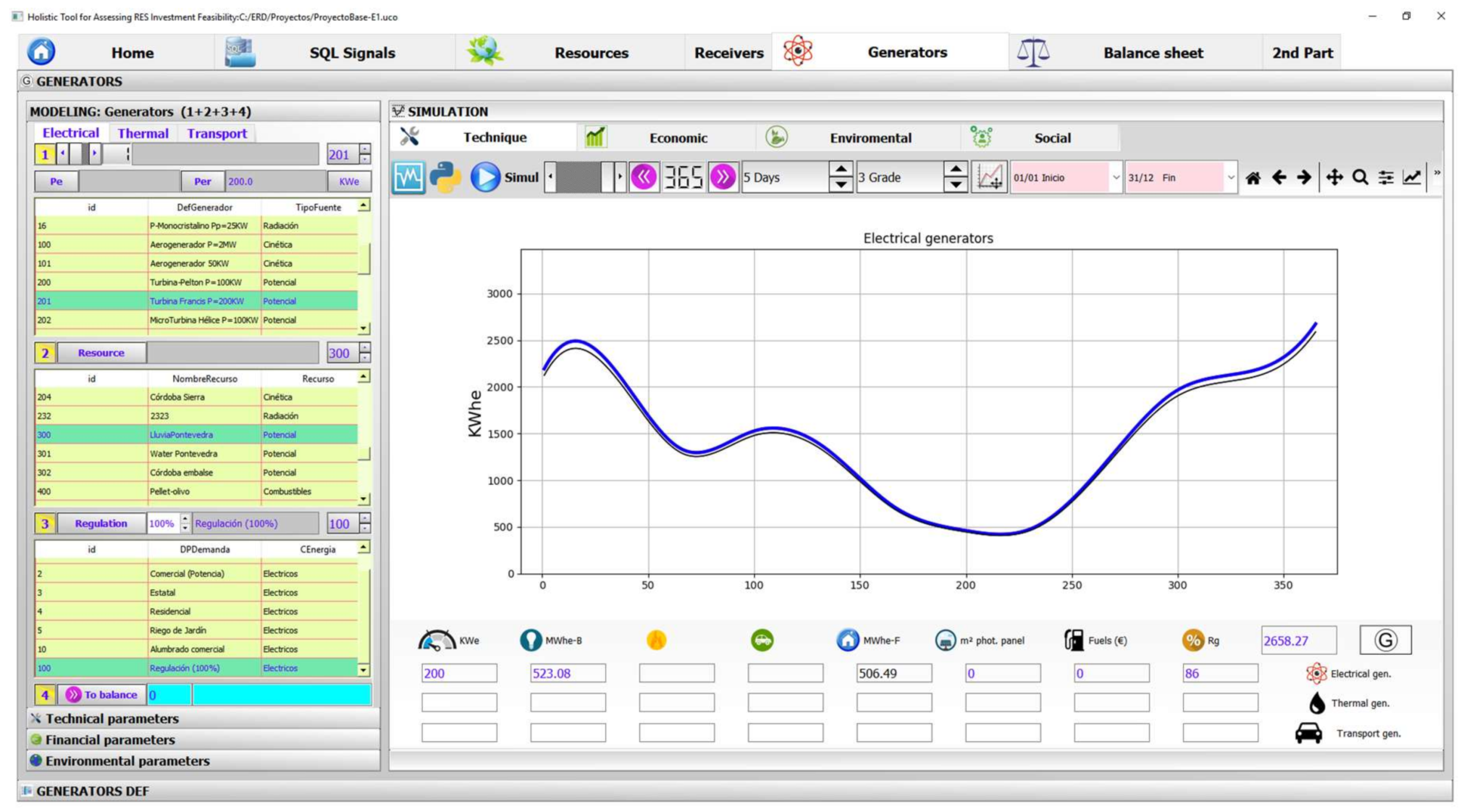
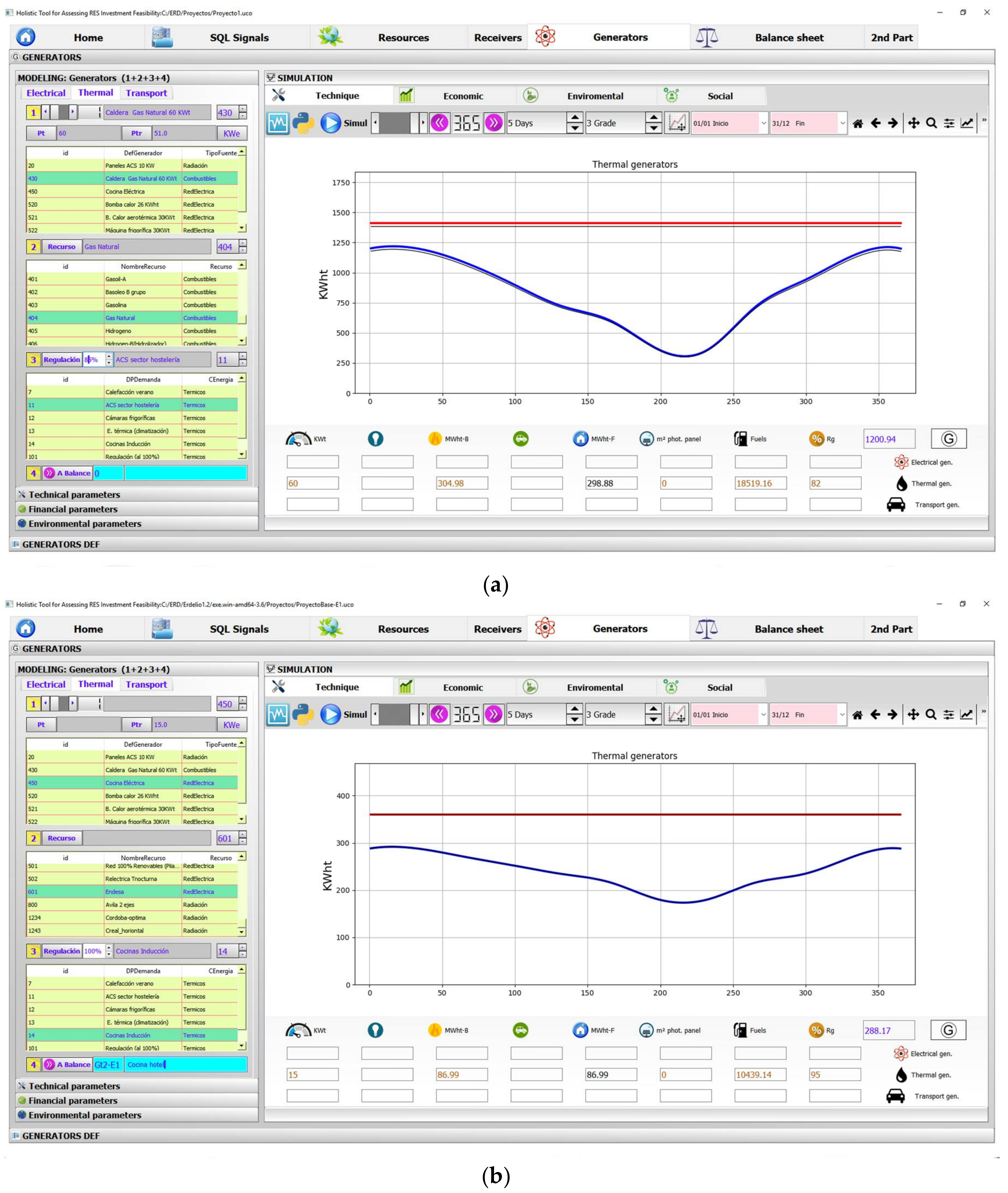
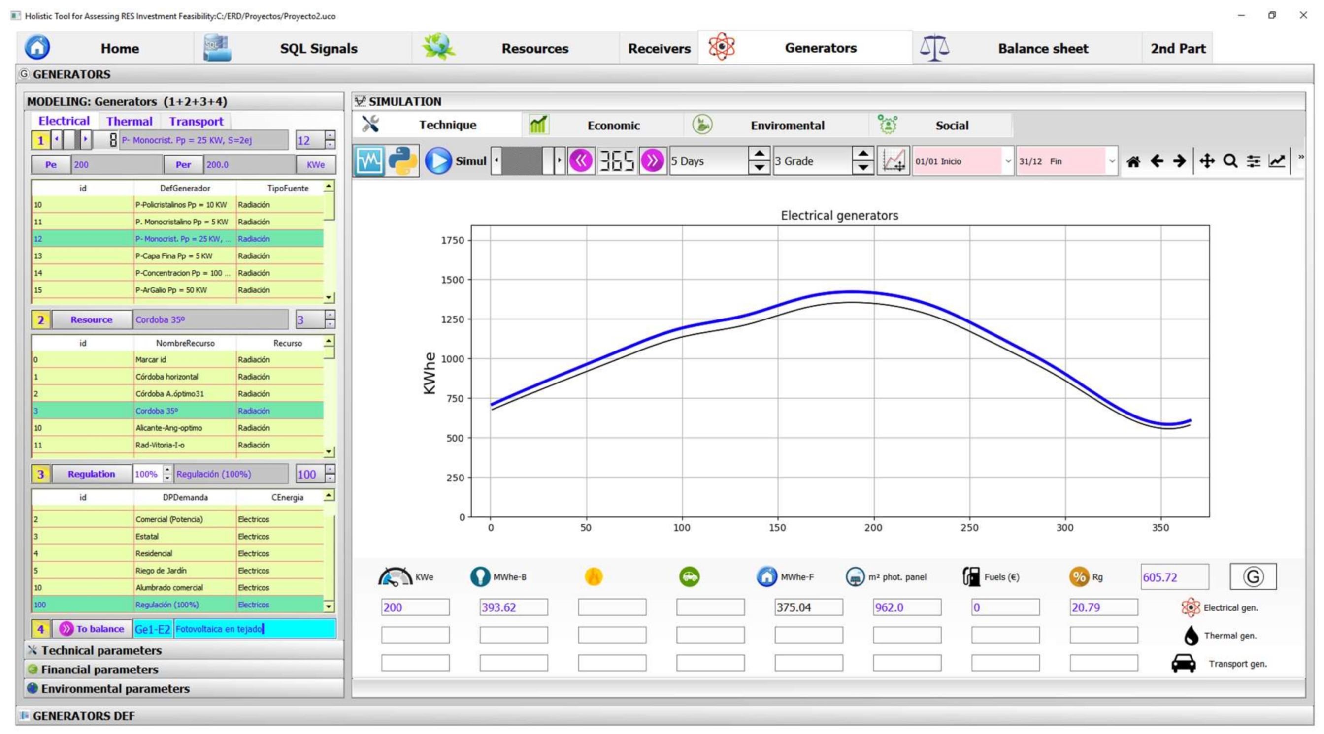
3.2. Generation Profiling Tab
3.2.1. Technical Feasibility
3.2.2. Economic Viability
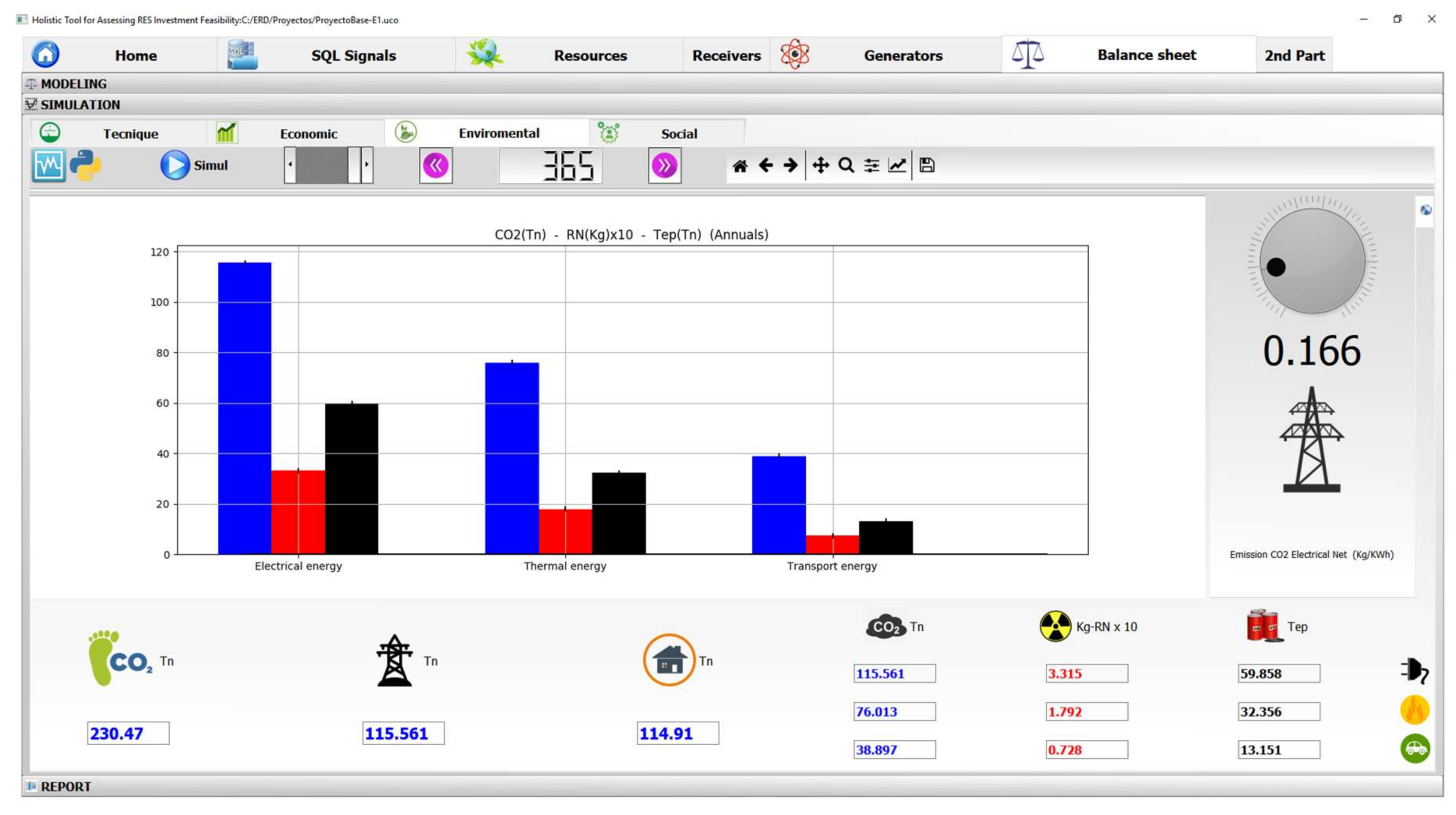
3.2.3. Environmental Viability
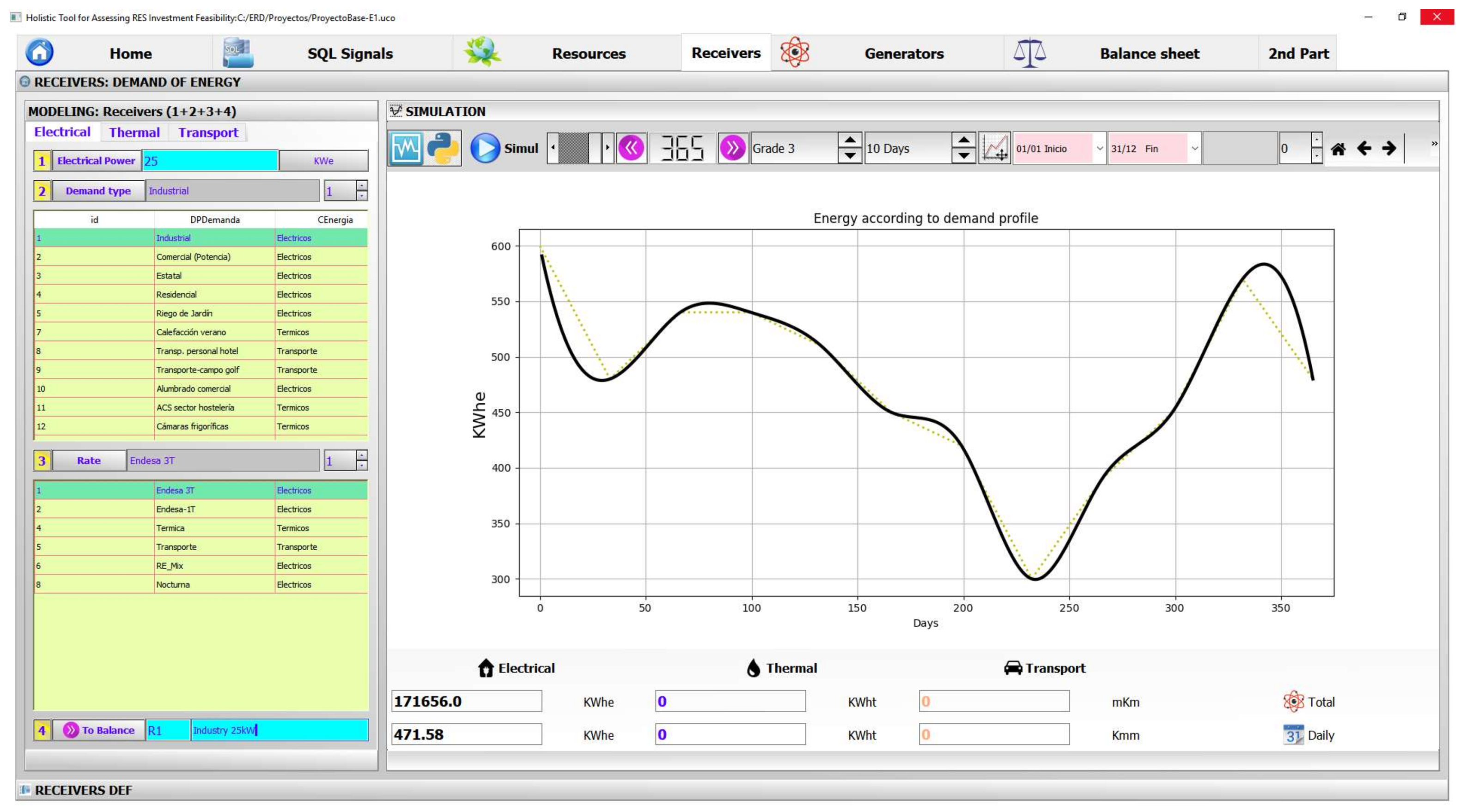
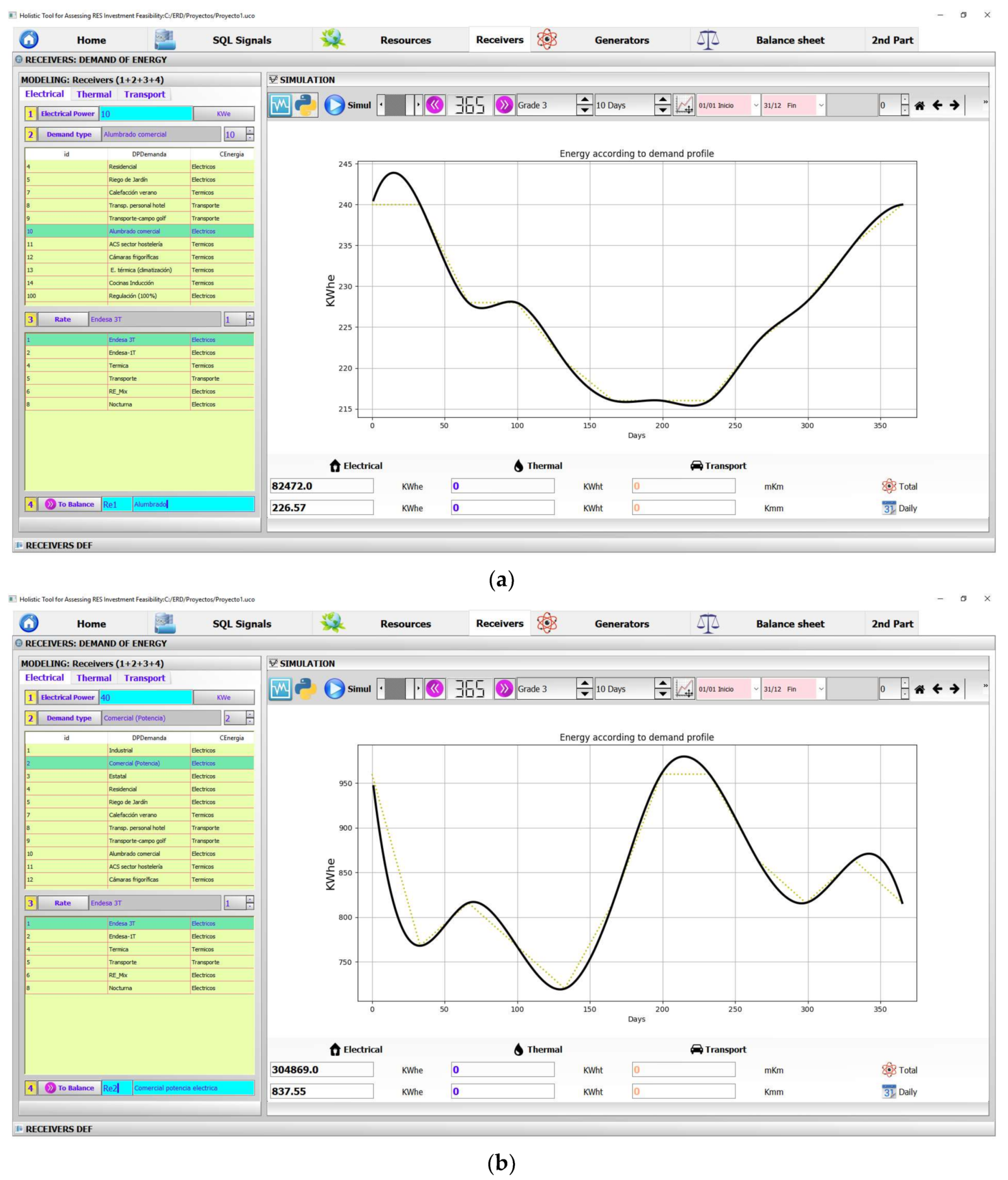
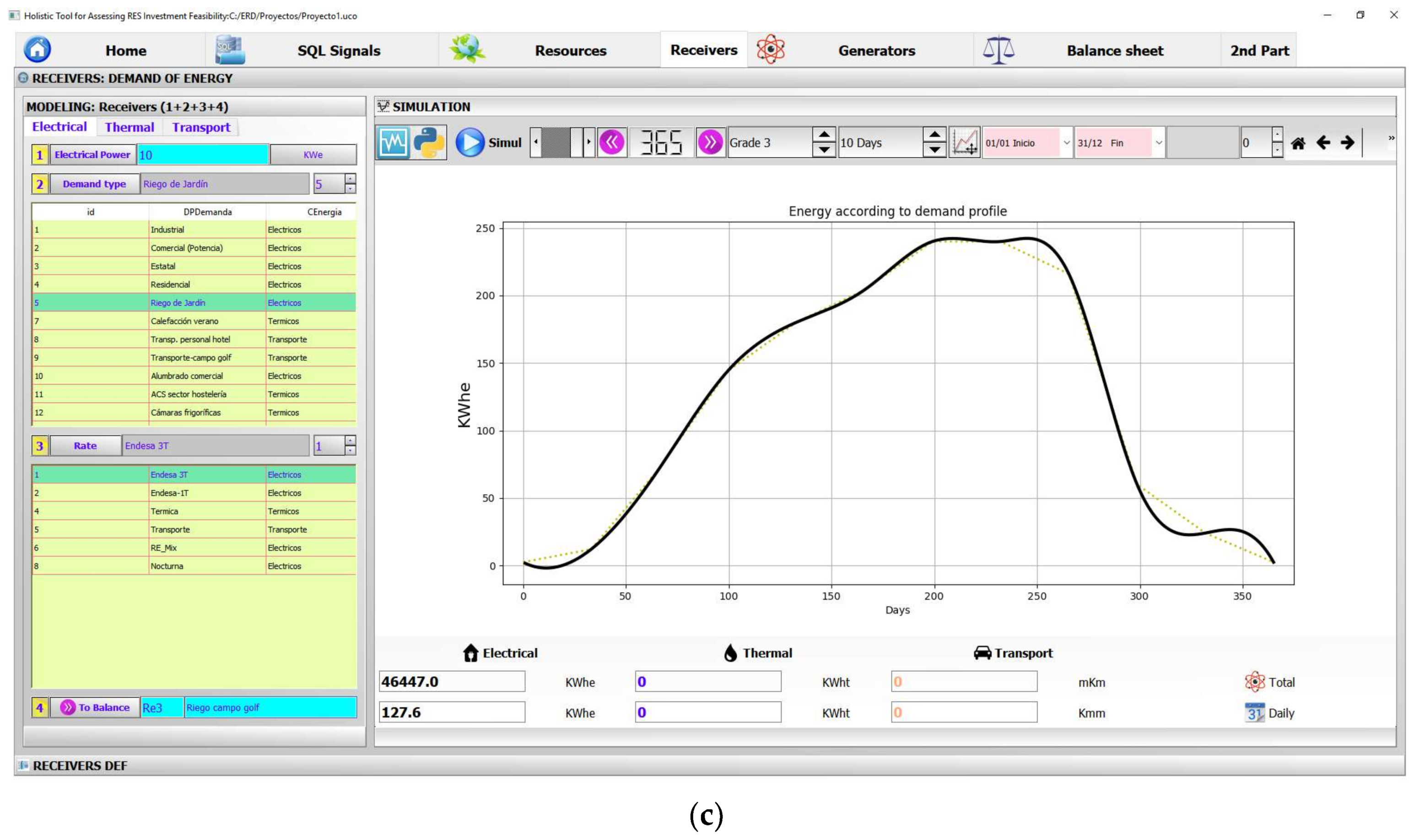
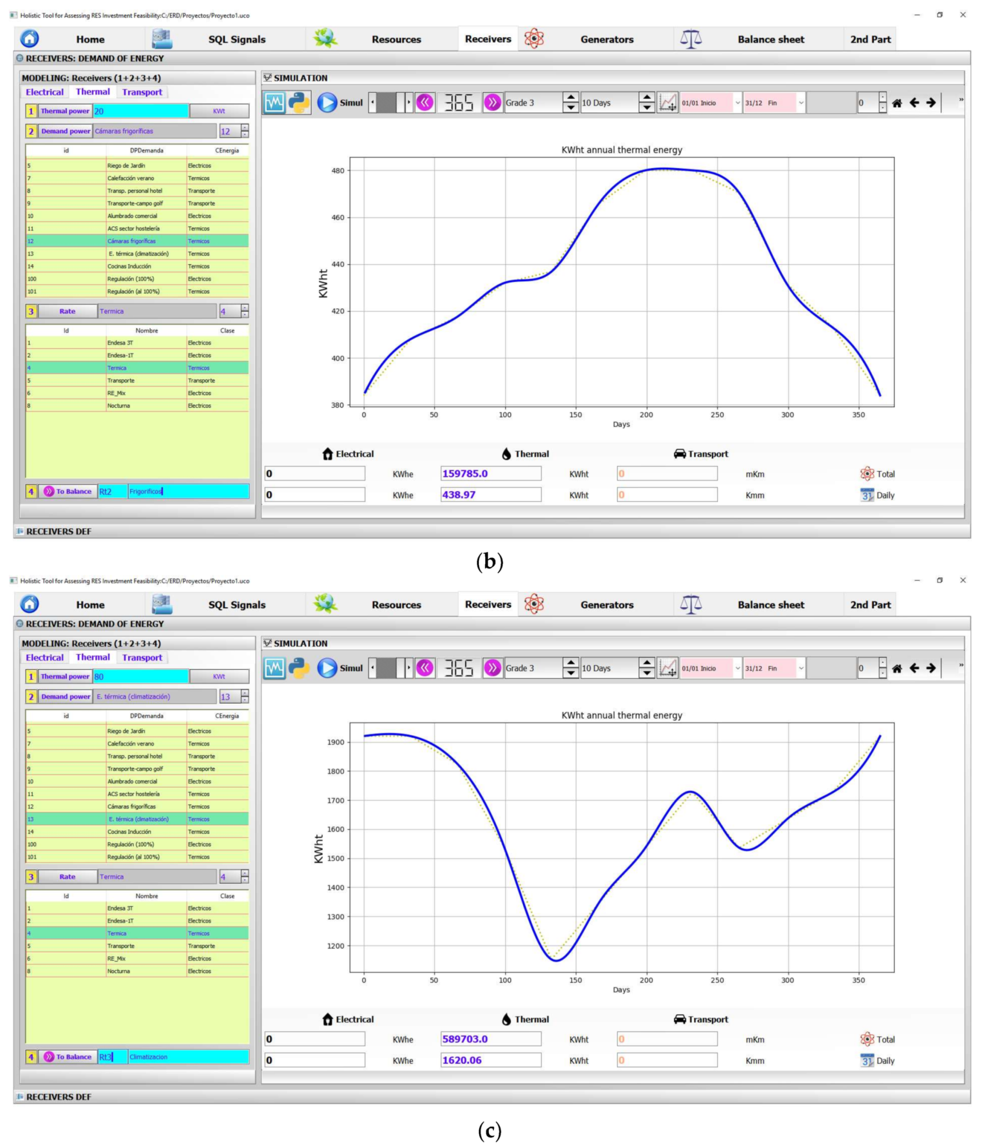
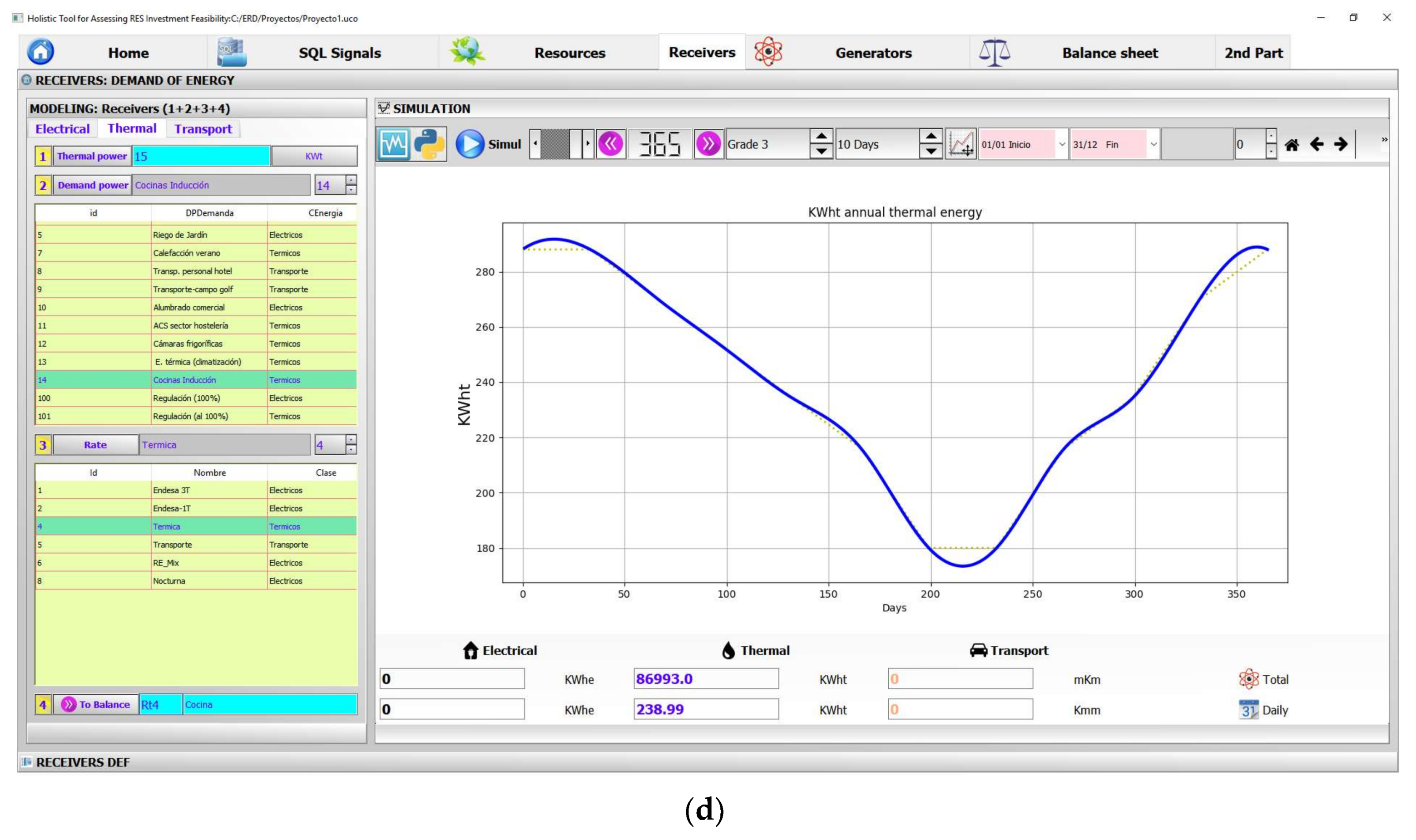
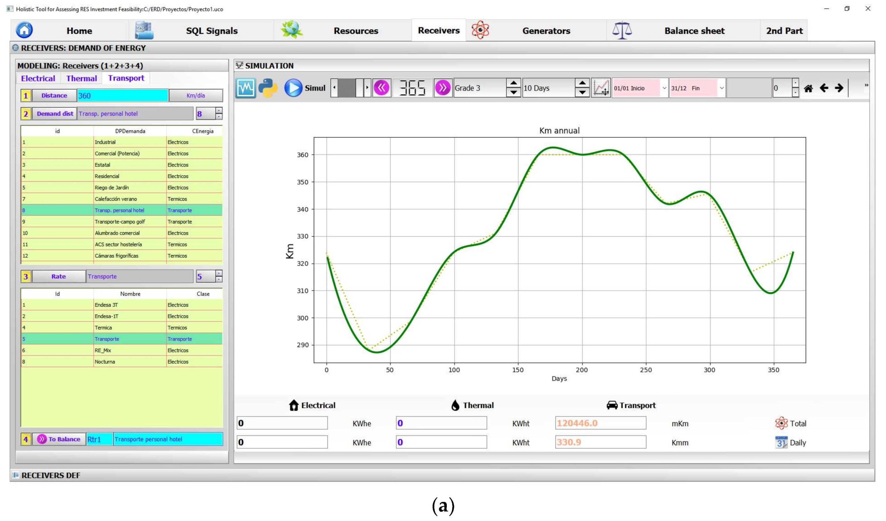
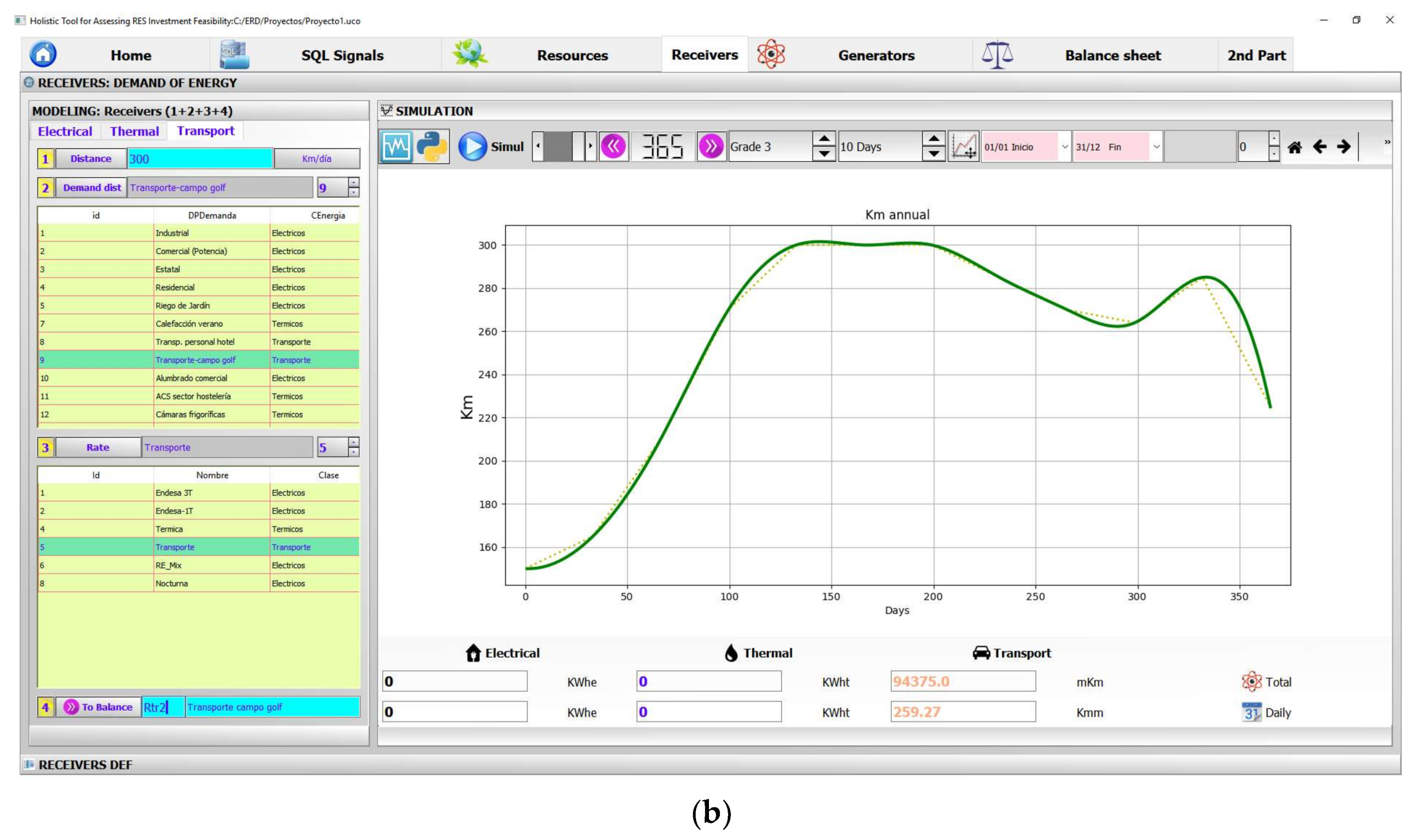
3.3. Demand Profile Modeling
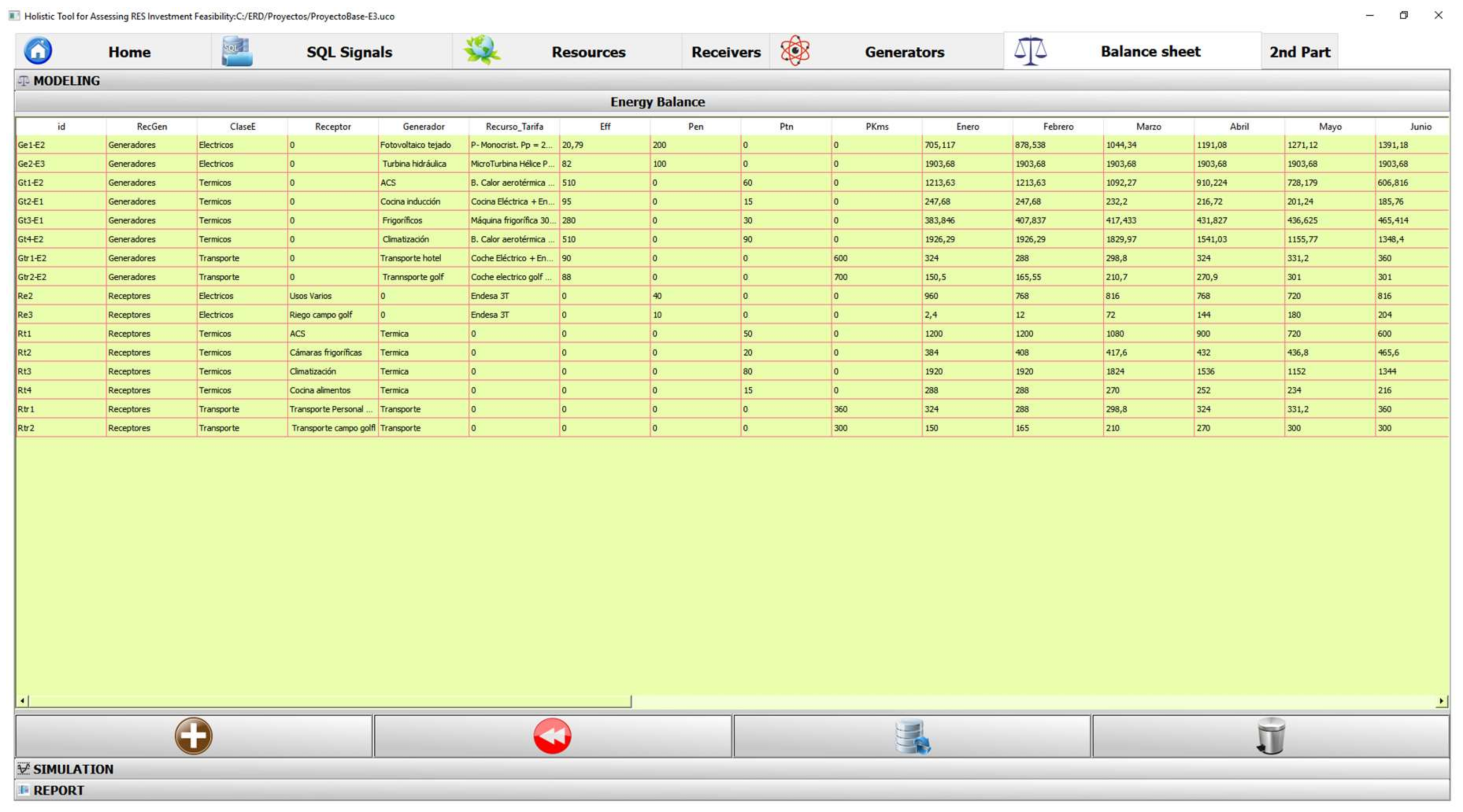
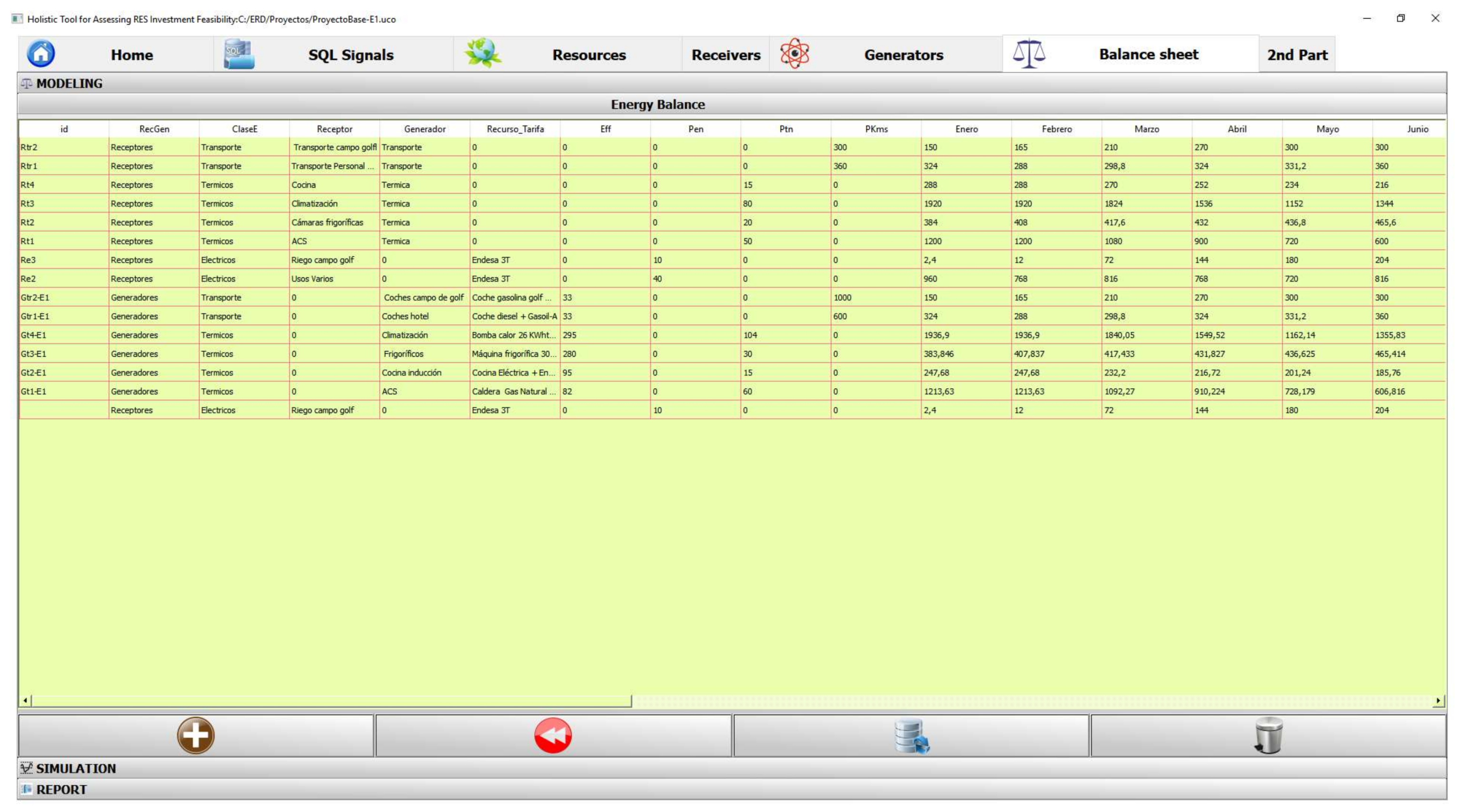
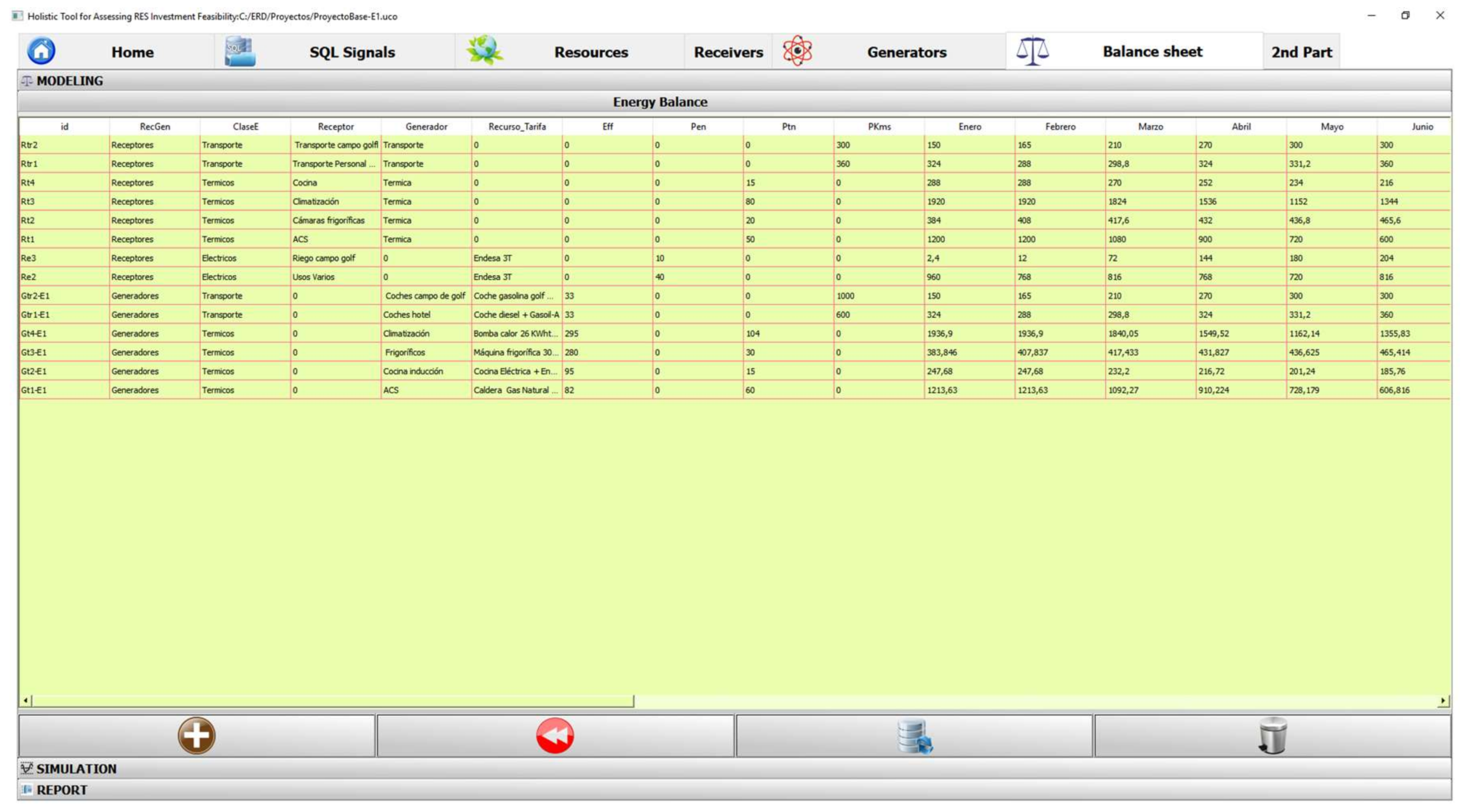
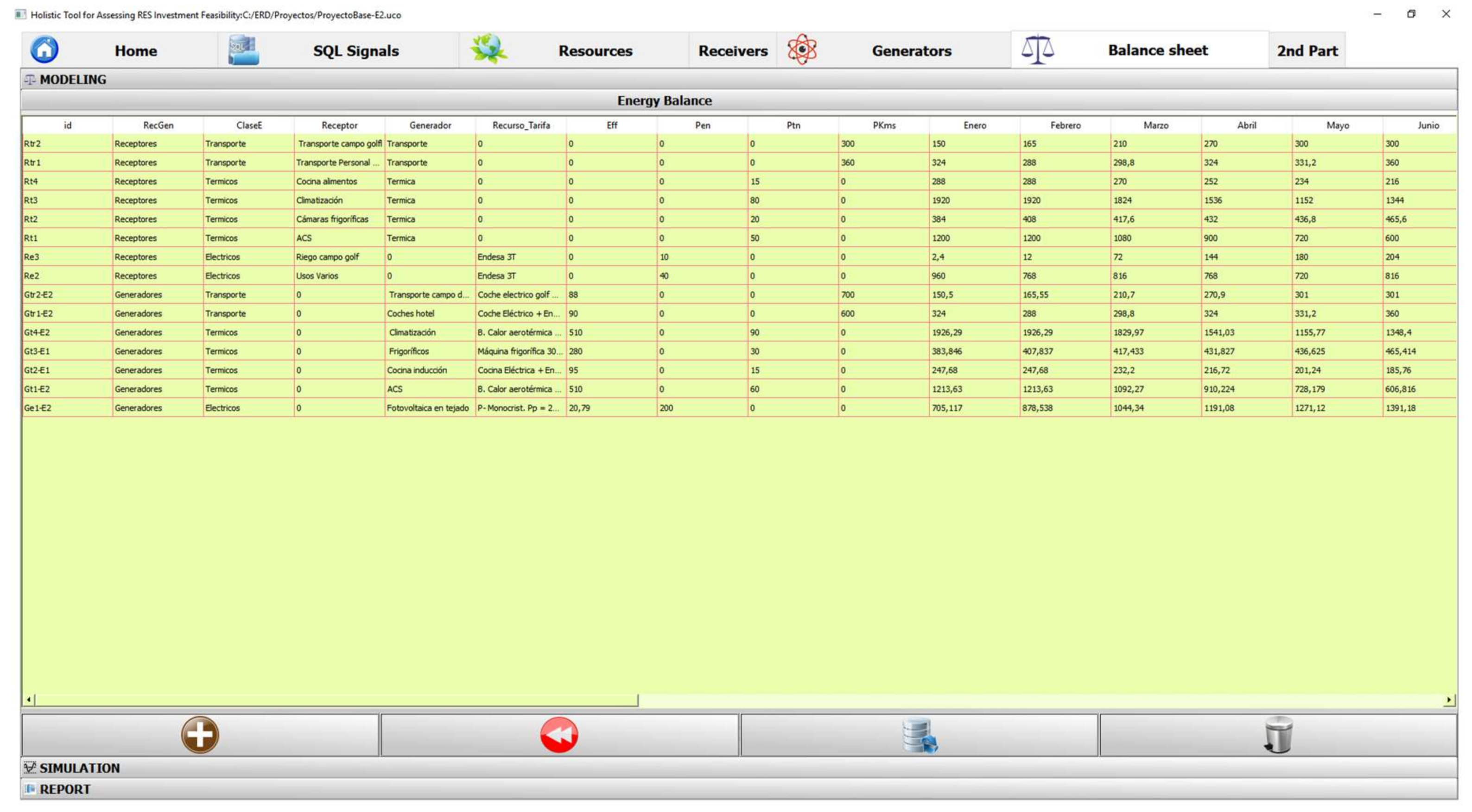
3.4. Energy Balance Calculation
4. An Illustrative Example of Application
4.1. Initial Settings
4.1.1. Overall Description
4.1.2. Choosing Demand Profiles
4.2. Analyzing Different Scenarios
4.2.1. Scenario 1
Constraints: choosing generators and their respective profiles
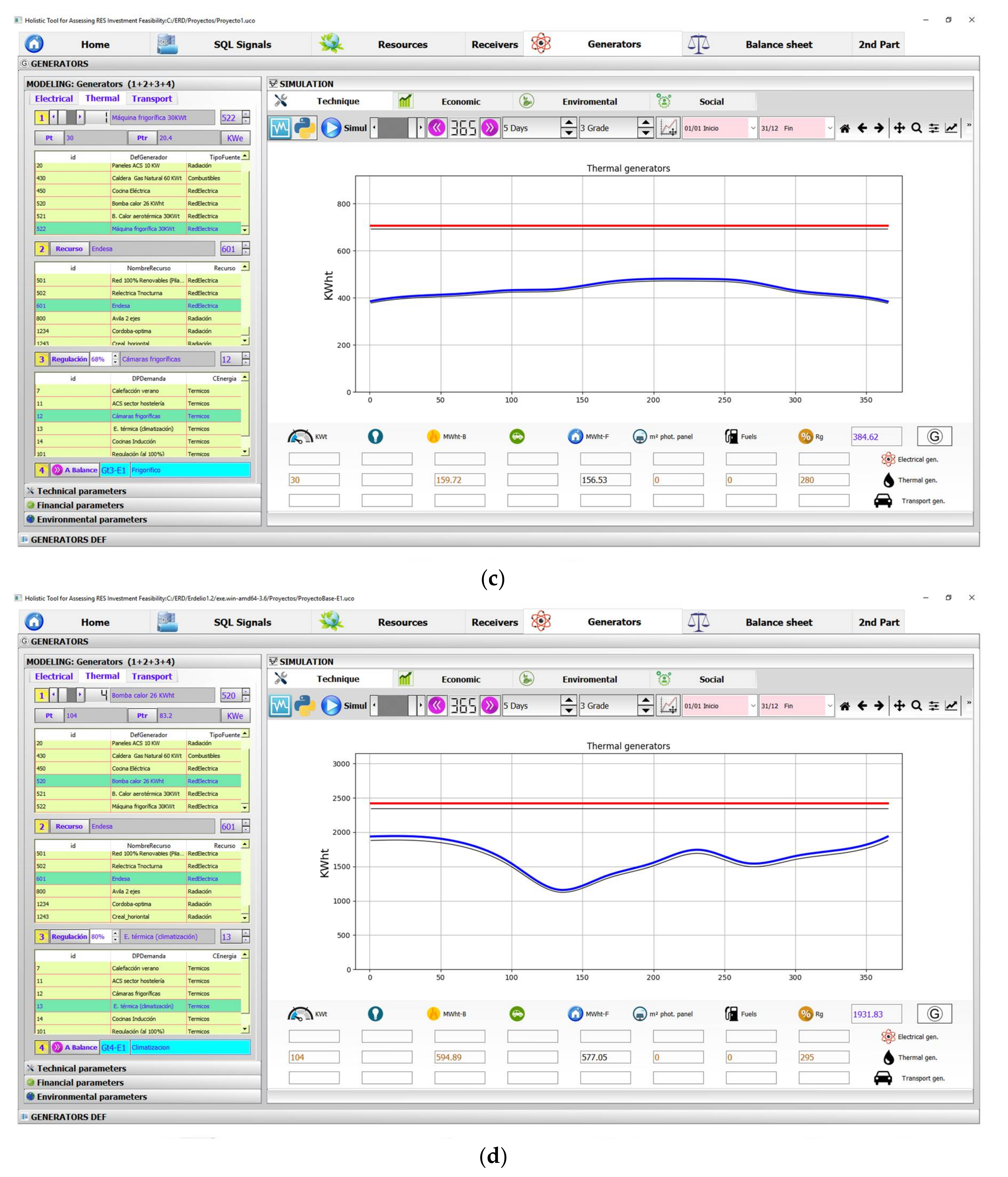
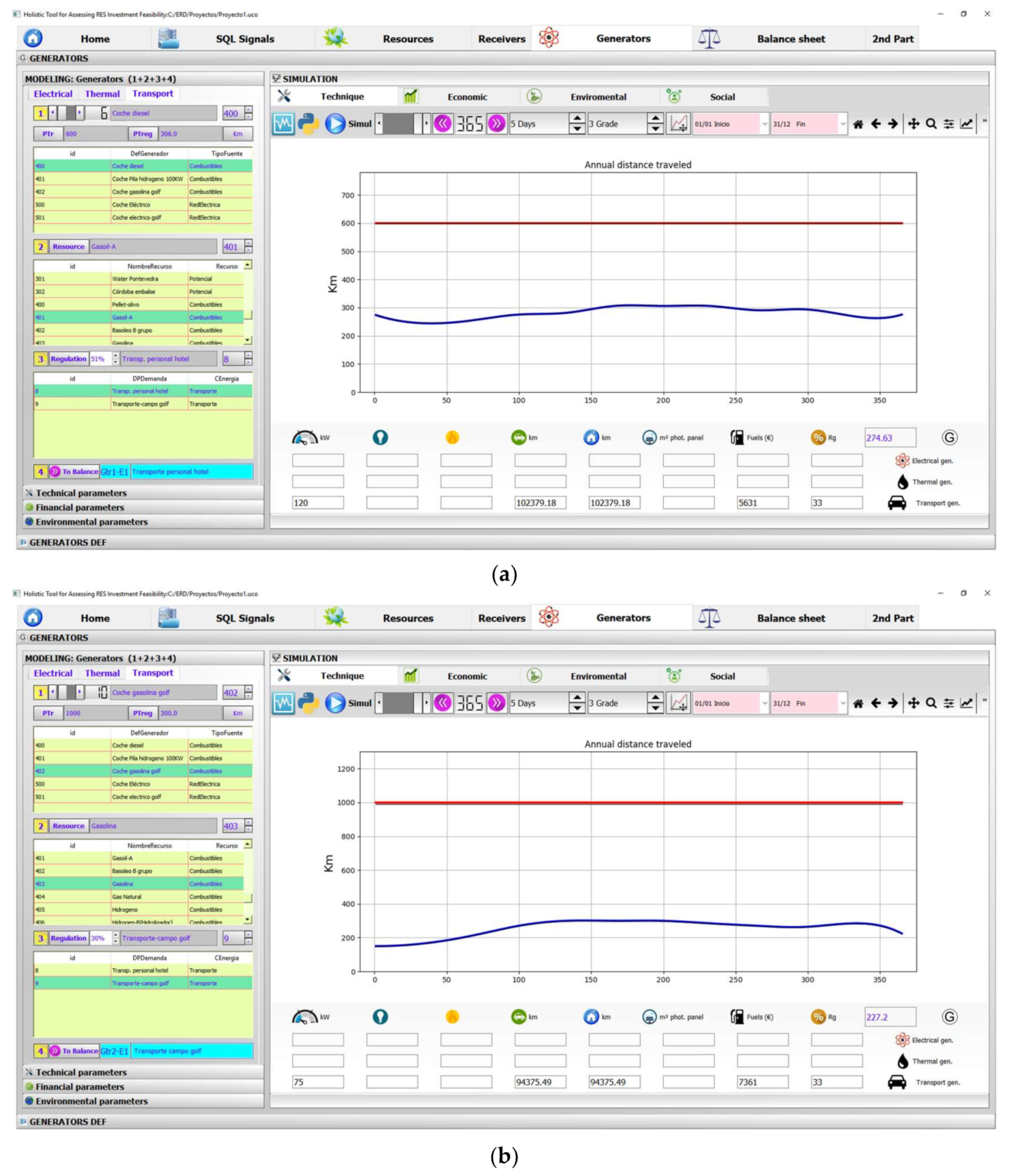
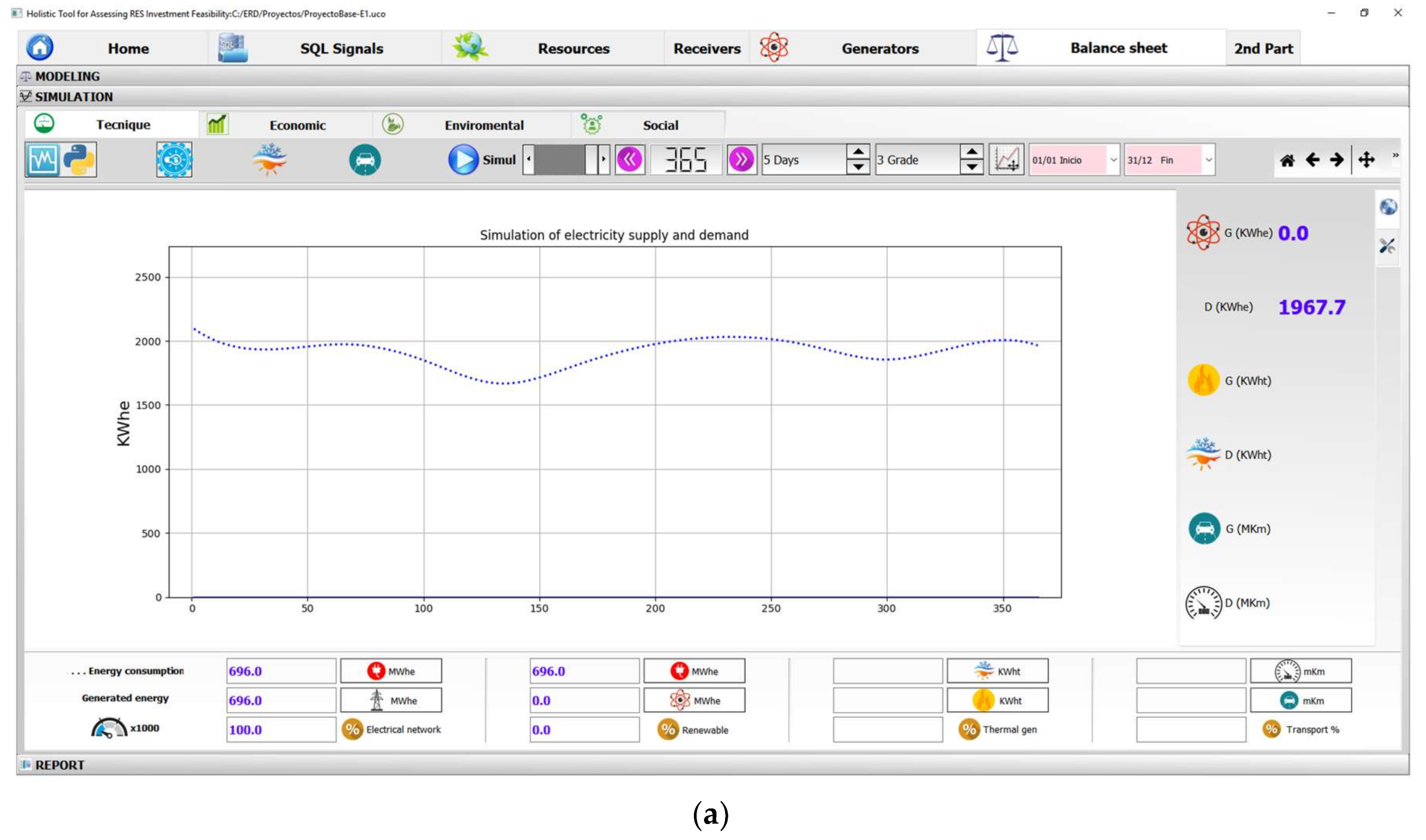
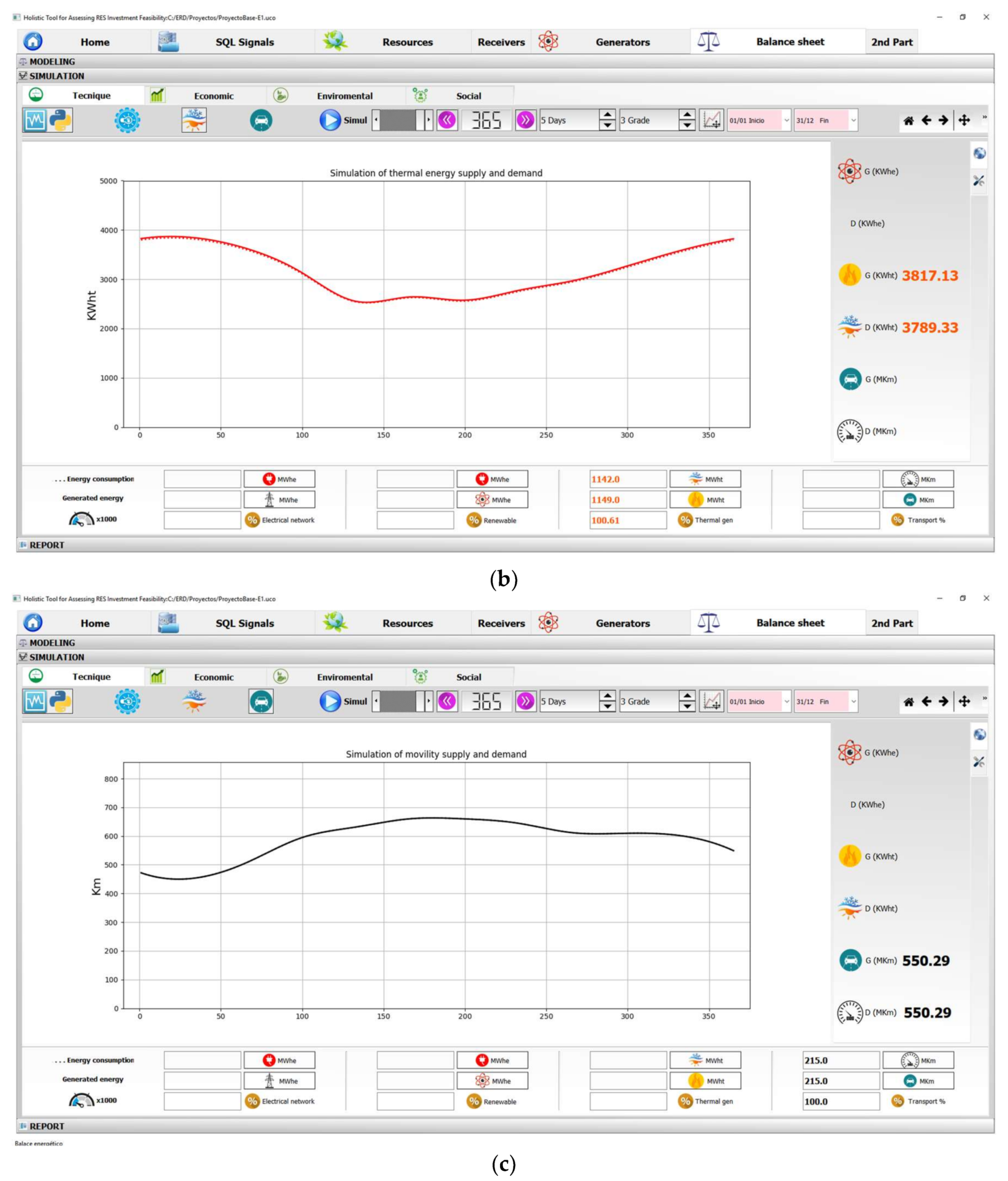
Technical Analysis
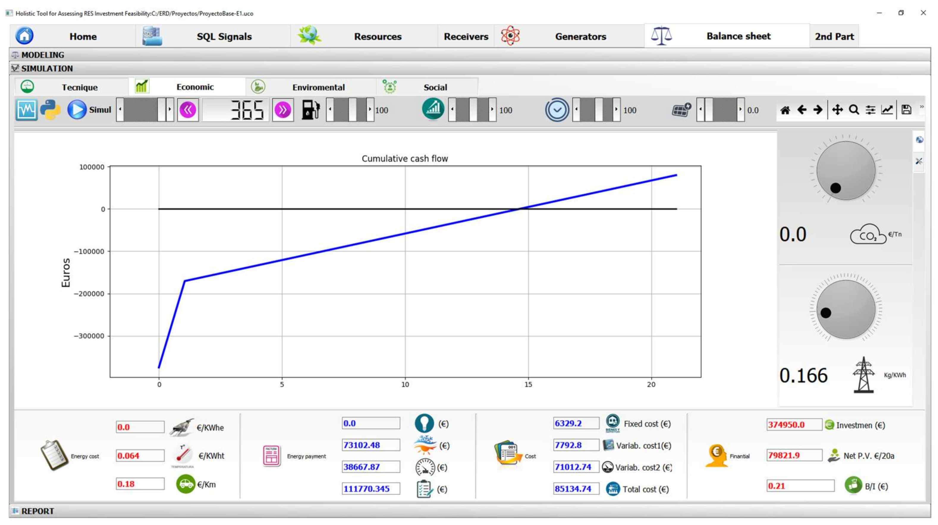
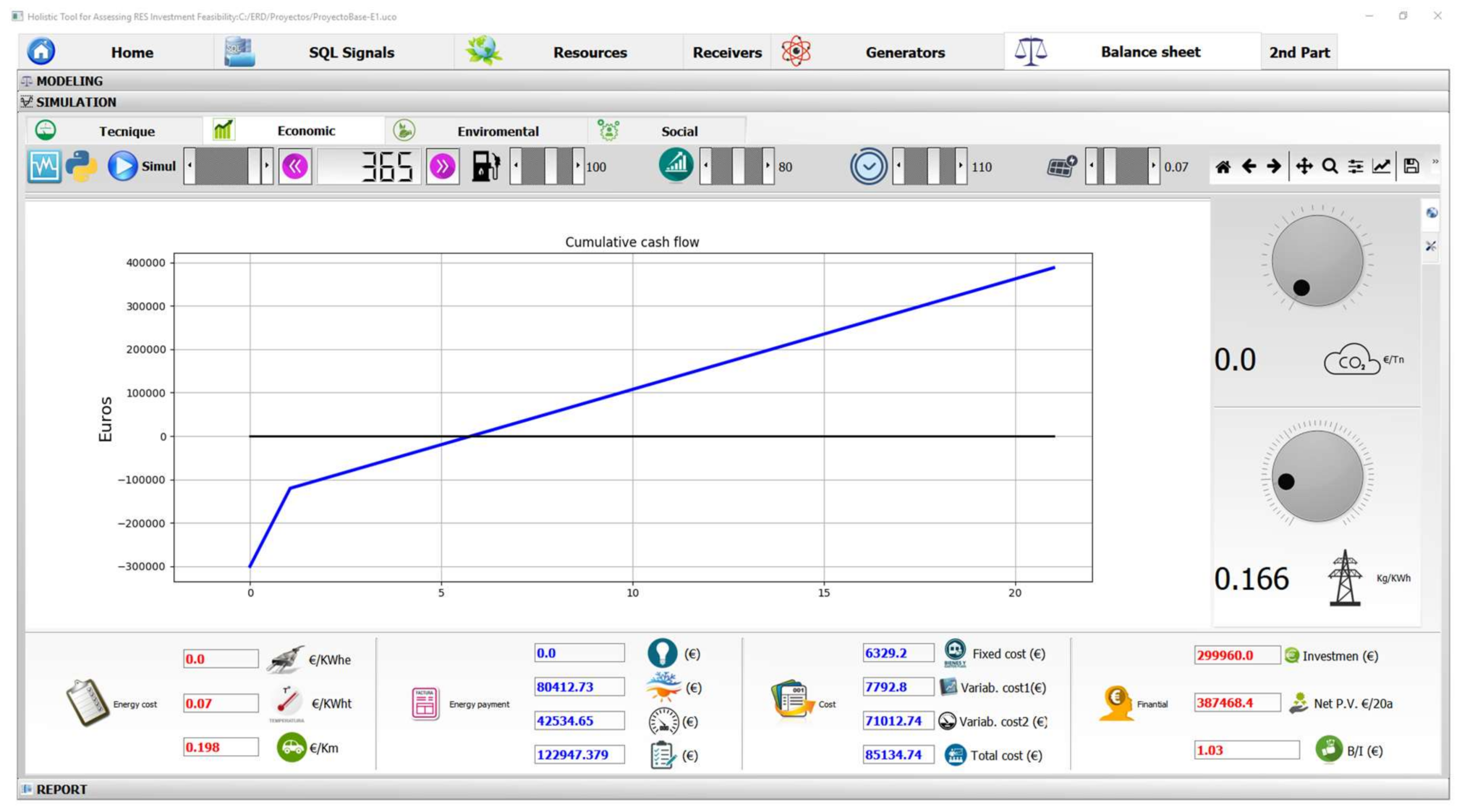
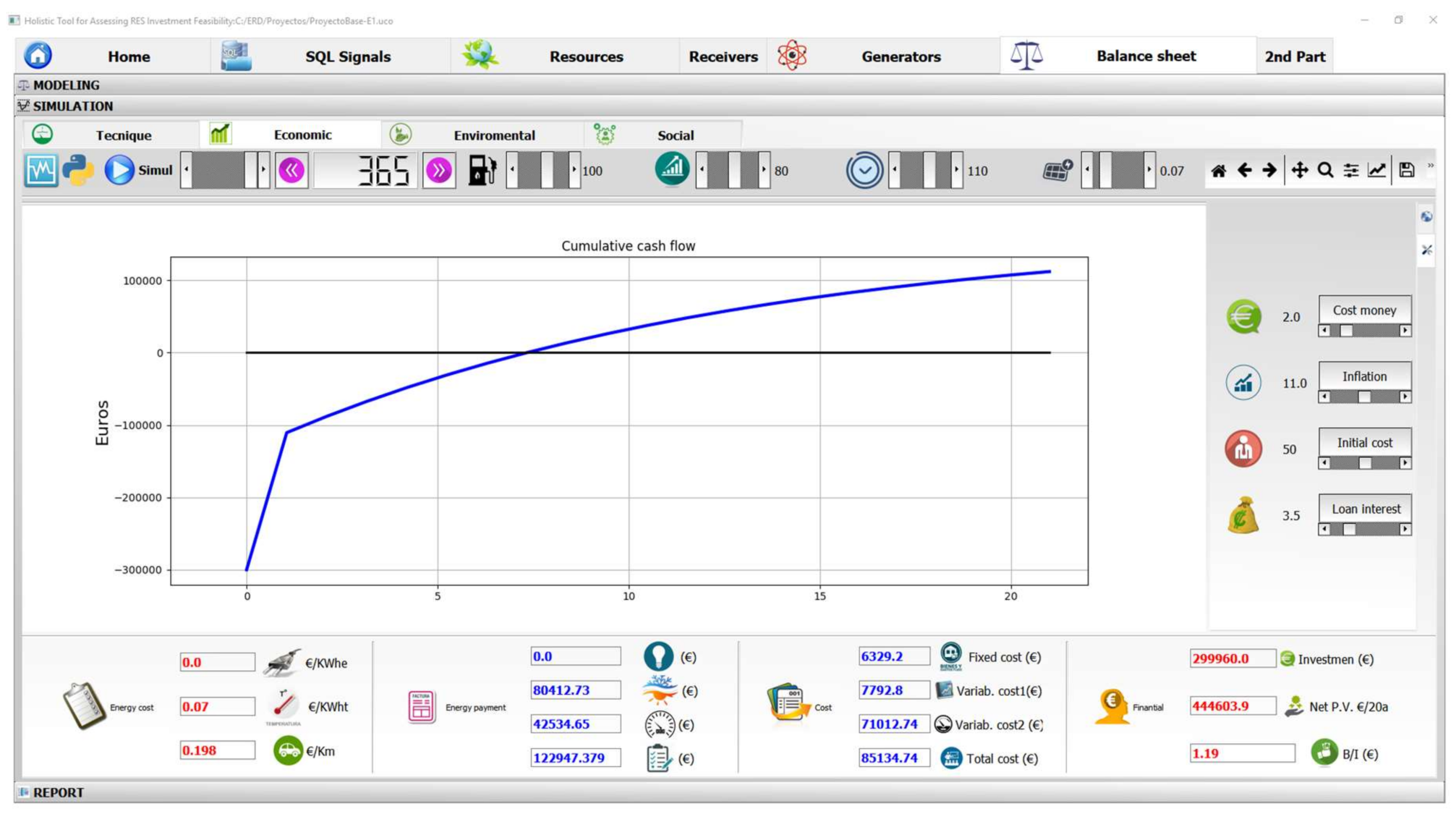
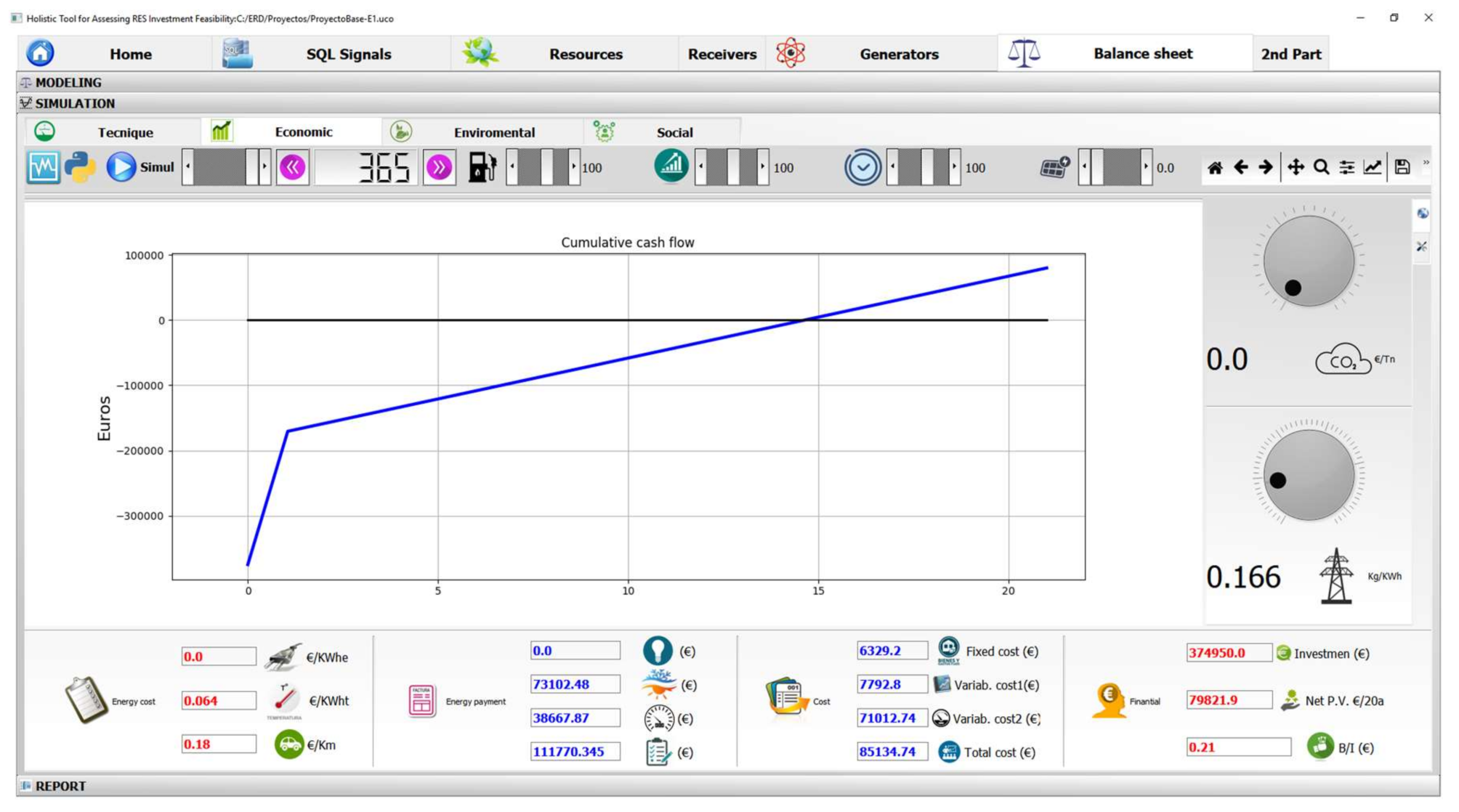
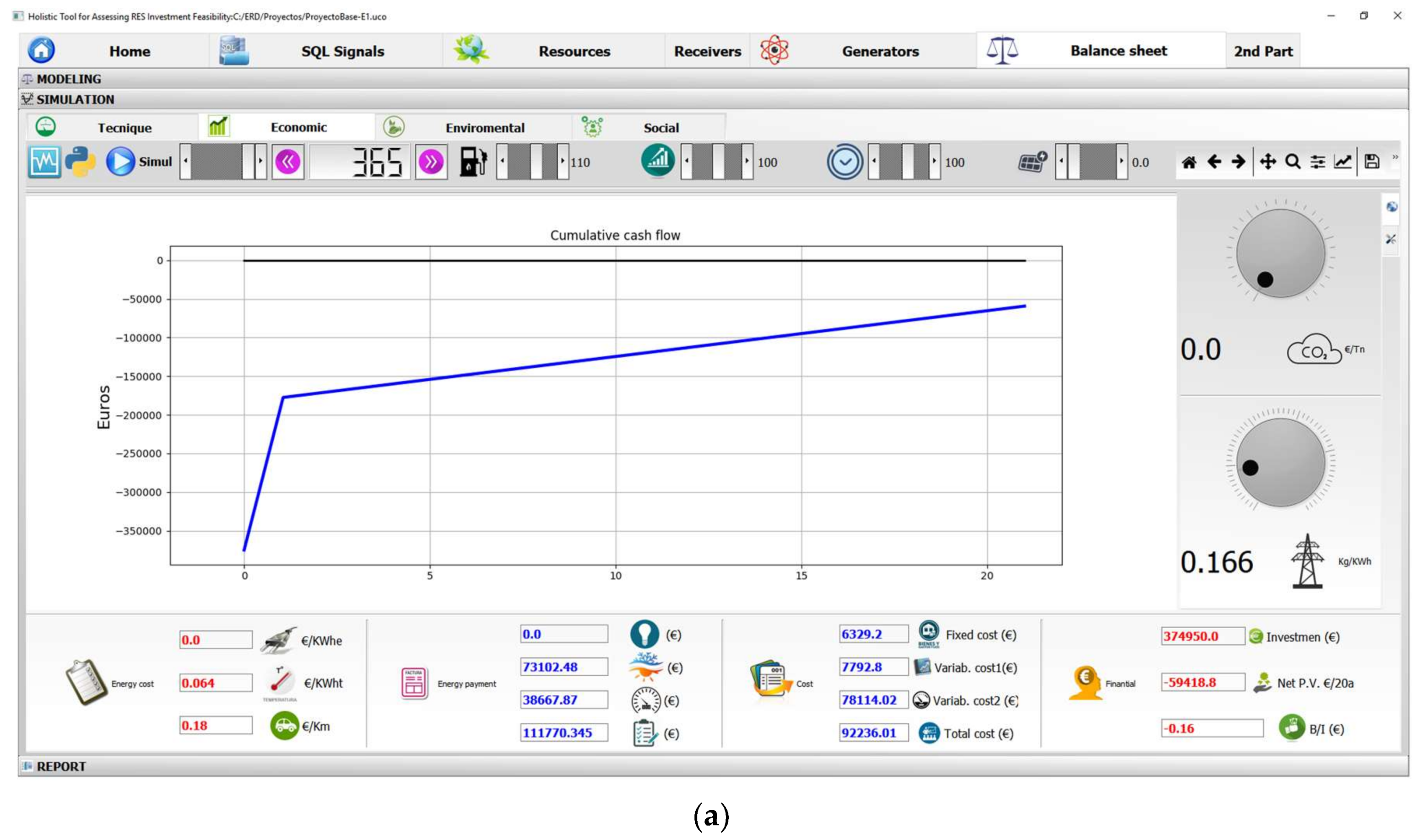
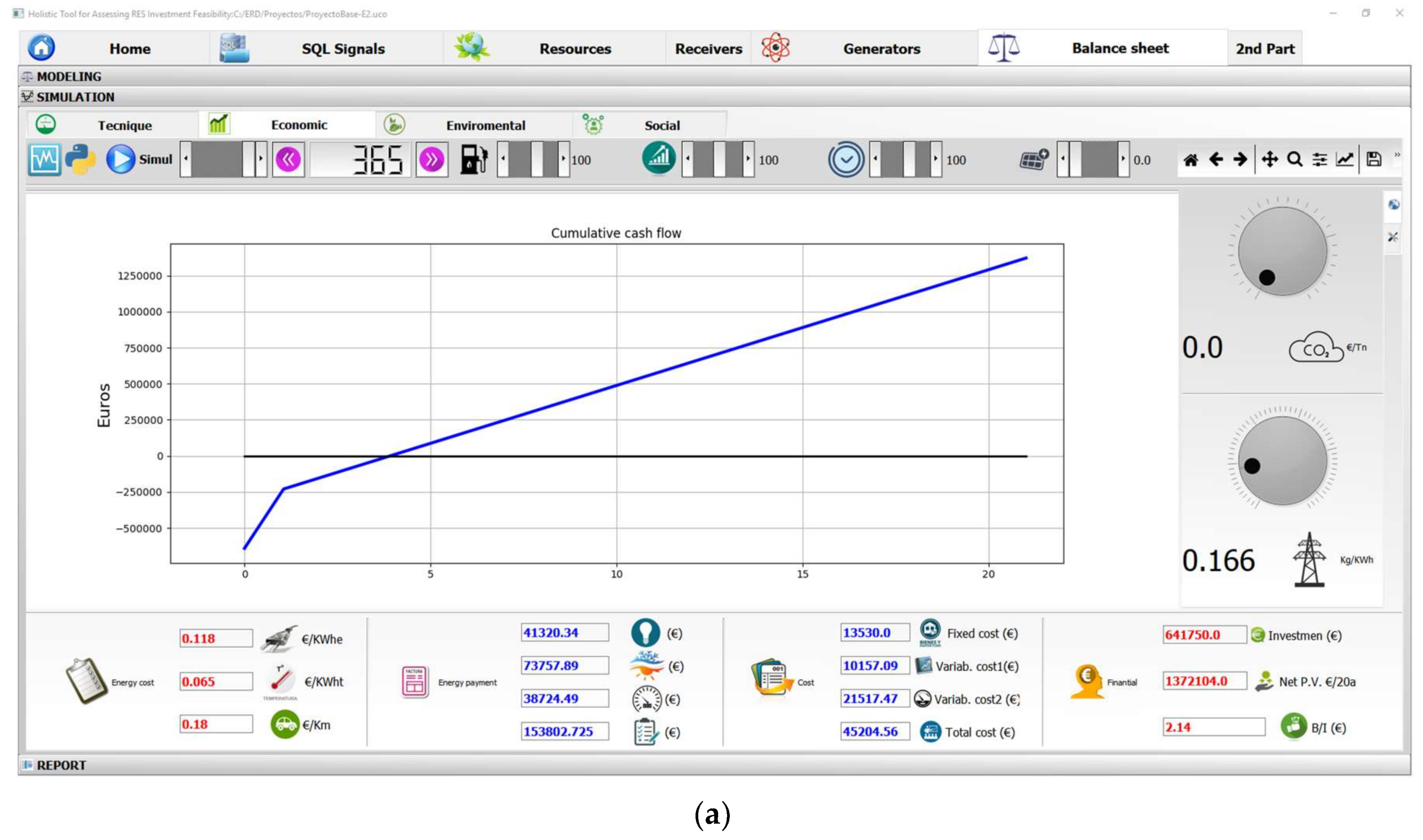
Economic Analysis
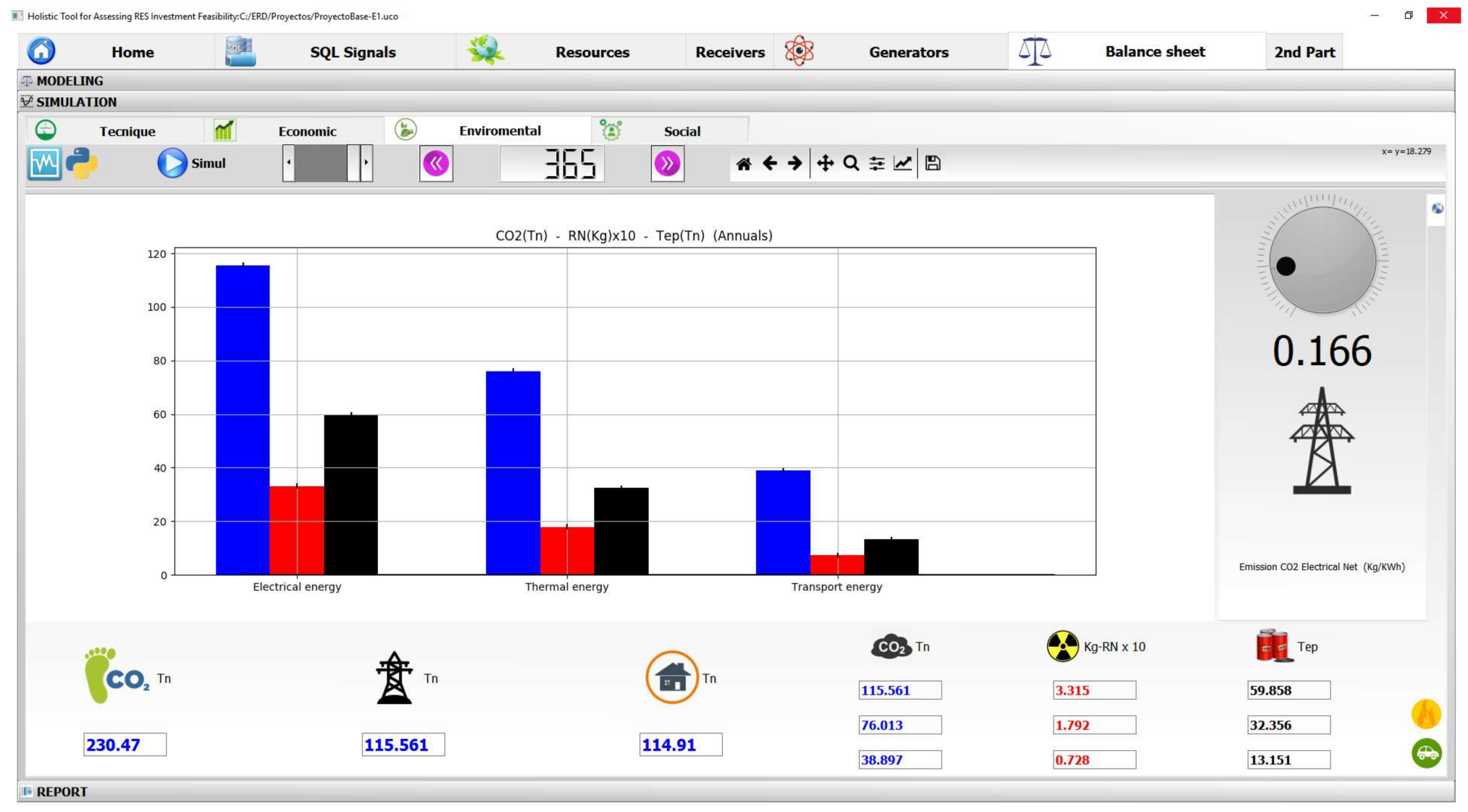
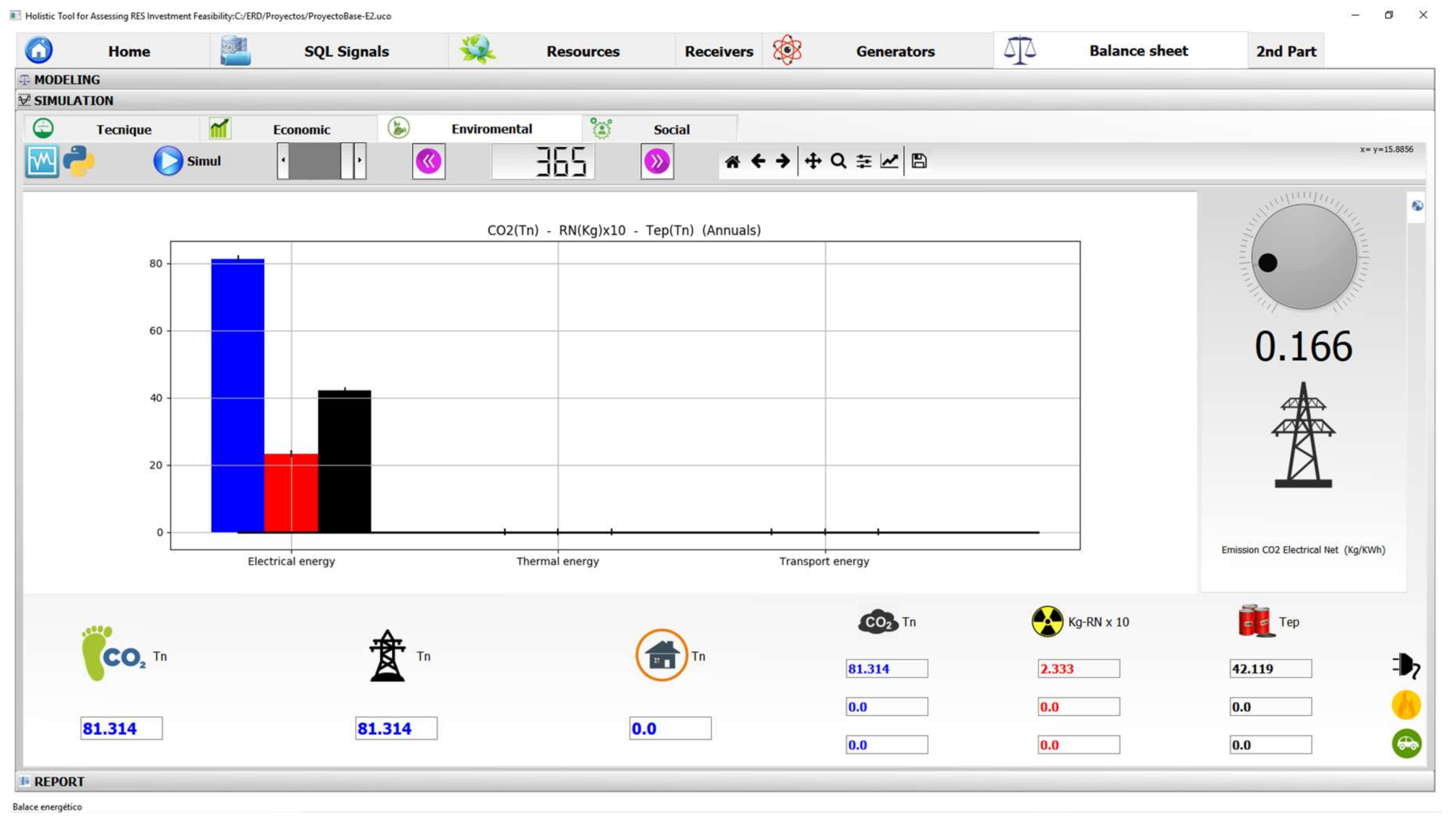
Environmental Analysis
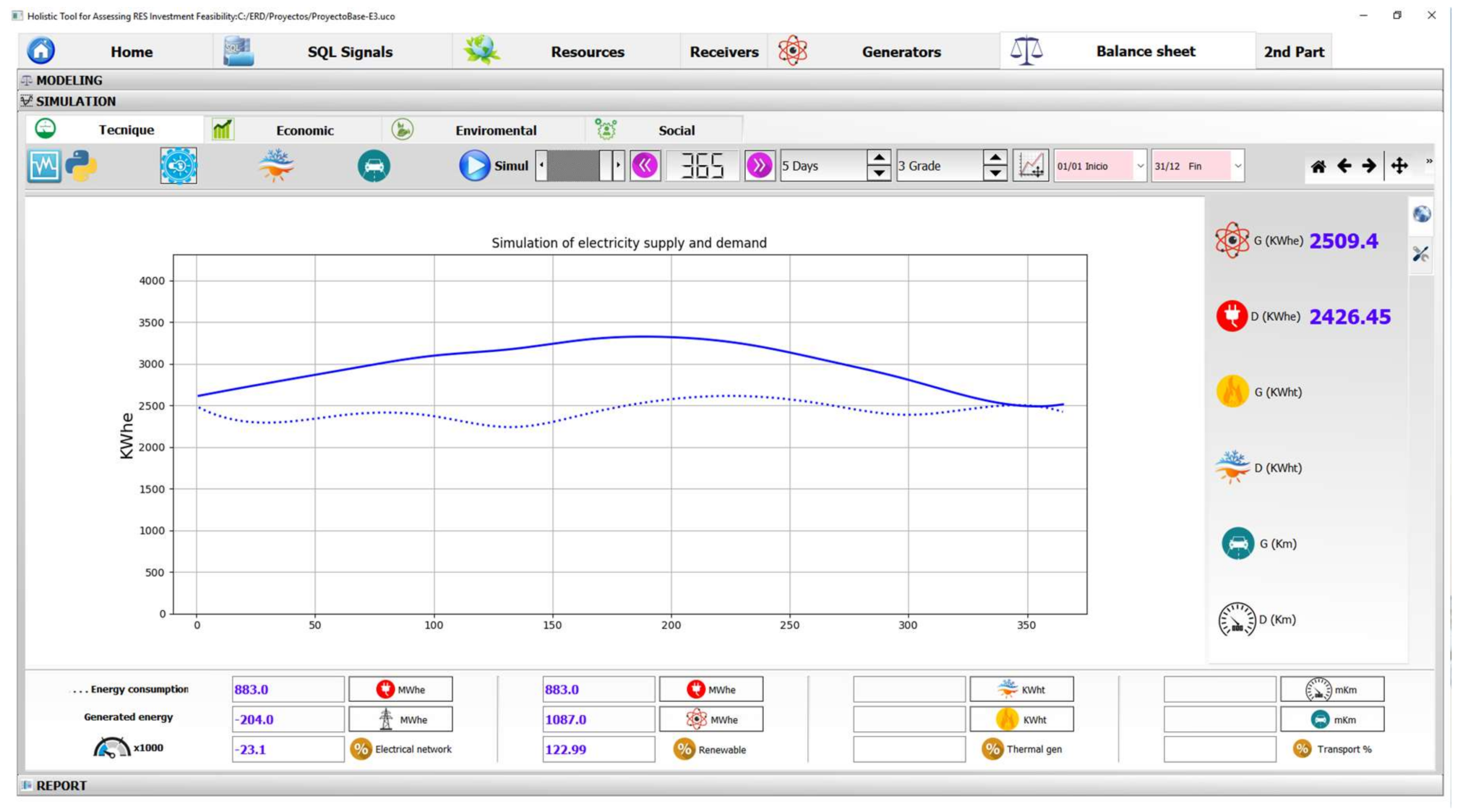
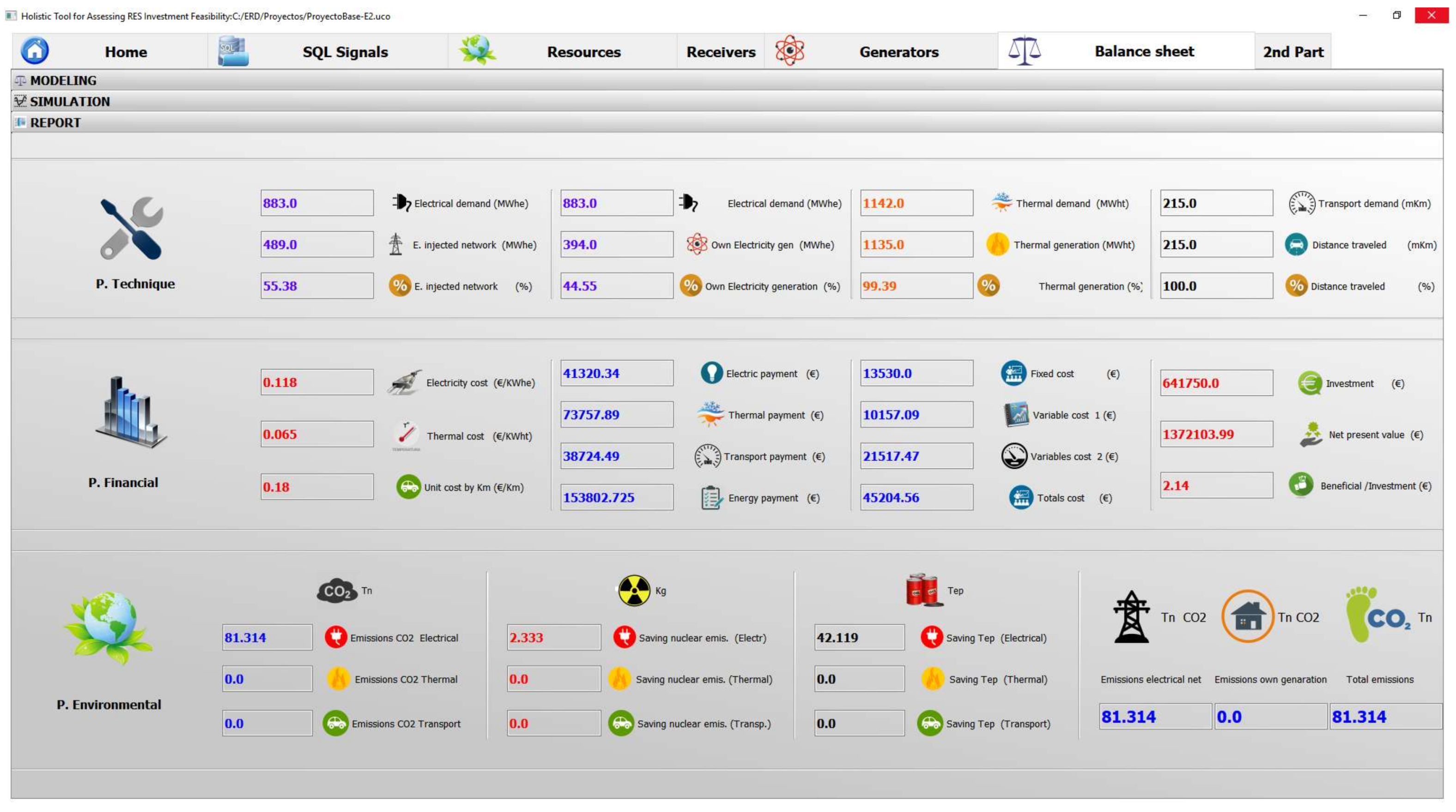
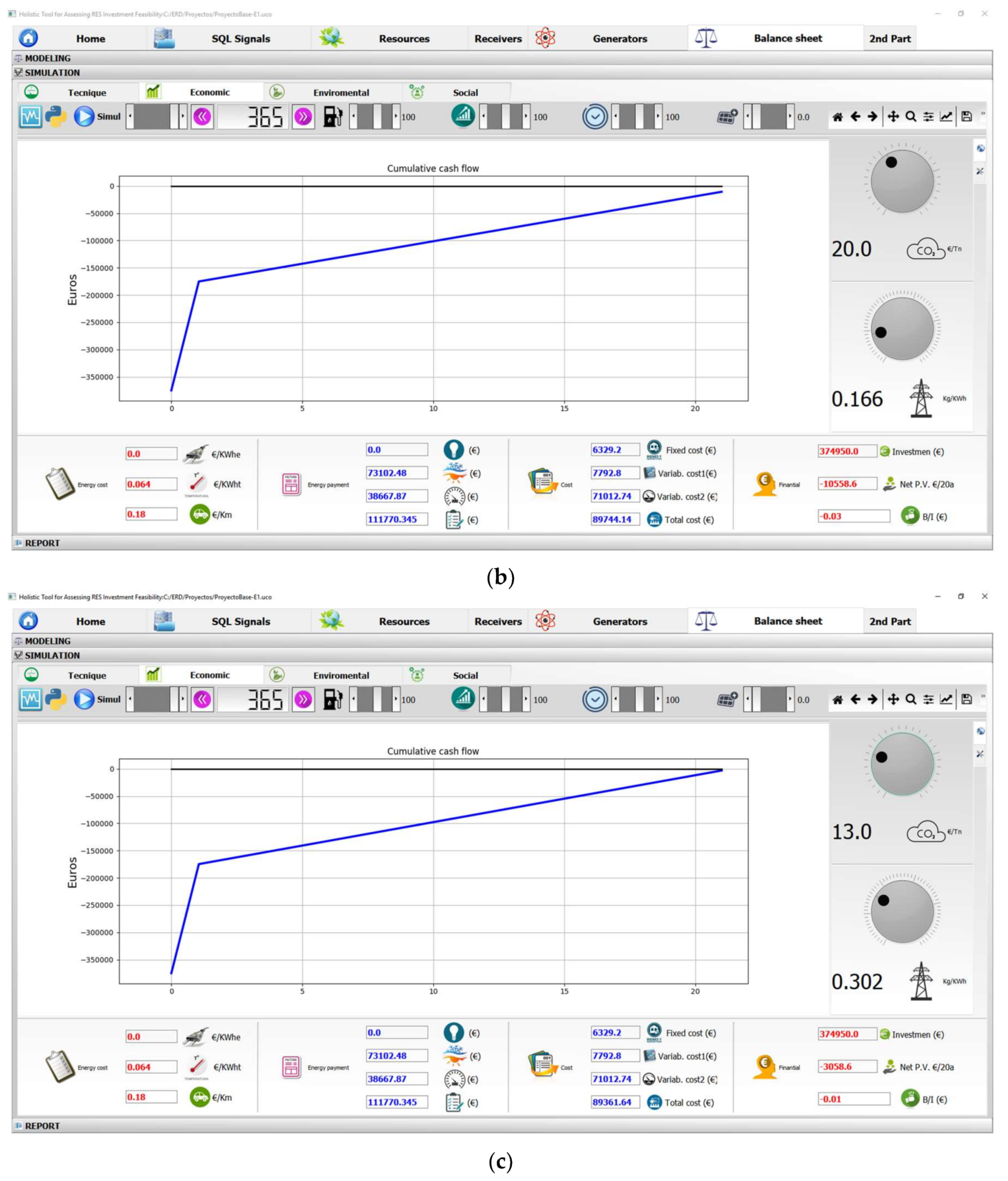
4.2.2. Scenario 2
5. Conclusions
Author Contributions
Conflicts of Interest
References
- Salom, J.; Marszal, A.J.; Widén, J.; Candanedo, J.; Lindberg, K.B. Analysis of load match and grid interaction indicators in net zero energy buildings with simulated and monitored data. Appl. Energy 2014, 136, 119–131. [Google Scholar] [CrossRef]
- Palacios-Garcia, E.J.; Moreno-Munoz, A.; Santiago, I.; Moreno-Garcia, I.M.; Milanés-Montero, M.I. Smart community load matching using stochastic demand modeling and historical production data. In Proceedings of the 2016 IEEE 16th International Conference on Environment and Electrical Engineering (EEEIC), Florence, Italy, 6–8 June 2016; pp. 1–6. [Google Scholar]
- Kavgic, M.; Mavrogianni, A.; Mumovic, D.; Summerfield, A.; Stevanovic, Z.; Djurovic-Petrovic, M. A review of bottom-up building stock models for energy consumption in the residential sector. Build. Environ. 2010, 45, 1683–1697. [Google Scholar] [CrossRef]
- Short, W.; Packey, D.J.; Holt, T.; U.S. Department of Energy. A Manual for the Economic Evaluation of Energy Efficiency and Renewable Energy Technologies; No. NREL/TP--462-5173; National Renewable Energy Lab: Golden, CO, USA, 1995.
- Suganthi, L.; Samuel, A.A. Energy models for demand forecasting—A review. Renew. Sustain. Energy Rev. 2012, 16, 1223–1240. [Google Scholar] [CrossRef]
- Solar-Estimate, Solar Calculator. Available online: http://www.solar-estimate.org (accessed on 30 November 2017).
- EC. Institute for Energy and Transport, Photovoltaic Geographical Information System (PVGIS). 2010. Available online: http://re.jrc.ec.europa.eu/pvgis/apps4/pvest.php (accessed on 15 August 2017).
- Energy Saving Trust. Tools and Calculators. Available online: http://www.energysavingtrust.org.uk/resources (accessed on 13 June 2017).
- National Renewable Energy Laboratory (NREL). Solar and Wind Energy Resource Assessment (SWERA) Model. 2016. Available online: www.nrel.gov/analysis/models_tools.html (accessed on 30 May 2017).
- Ciabattoni, L.; Grisostomi, M.; Ippoliti, G.; Longhi, S.; Mainardi, E. On line Solar Irradiation Forecasting by Minimal Resource Allocating Networks. In Proceedings of the 20th IEEE Mediterranean Conference on Control & Automation (MED 2012), Barcelona, Spain, 3–6 July 2012; pp. 1506–1511. [Google Scholar]
- Ameli, S.M.; Agnew, B.; Potts, I. Integrated distributed energy evaluation software (IDEAS): Simulation of a micro-turbine based CHP system. Appl. Therm. Eng. 2007, 27, 2161–2165. [Google Scholar] [CrossRef]
- Anastaselos, D.; Giama, E.; Papadopoulos, A.M. An assessment tool for the energy, economic and environmental evaluation of thermal insulation solutions. Energy Build. 2009, 41, 1165–1171. [Google Scholar] [CrossRef]
- Axelsson, E.; Harvey, S.; Berntsson, T. A tool for creating energy market scenarios for evaluation of investments in energy intensive industry. Energy 2009, 34, 2069–2074. [Google Scholar] [CrossRef]
- Grandjean, A.; Adnot, J.; Binet, G. A review and an analysis of the residential electric load curve models. Sustain. Energy Rev. 2012, 16, 6539–6565. [Google Scholar] [CrossRef]
- Swan, L.; Ugursal, V. Modeling of end-use energy consumption in the residential sector: A review of modeling techniques. Renew. Sustain. Energy Rev. 2009, 13, 1819–1835. [Google Scholar] [CrossRef]
- Richardson, I.; Thomson, M.; Infield, D.; Clifford, C. Domestic electricity use: A high-resolution energy demand model. Energy Build. 2010, 42, 1878–1887. [Google Scholar] [CrossRef] [Green Version]
- Widén, J.; Wäckelgård, E. A high-resolution stochastic model of domestic activity patterns and electricity demand. Appl. Energy 2010, 87, 1880–1892. [Google Scholar] [CrossRef]
- Palacios-Garcia, E.J.; Chen, A.; Santiago, I.; Bellido-Outeiriño, F.J.; Flores-Arias, J.M.; Moreno-Munoz, A. Stochastic model for lighting’s electricity consumption in the residential sector. Impact of energy saving actions. Energy Build. 2015, 89, 245–259. [Google Scholar] [CrossRef]
- Bellido-Outeirino, F.; Flores-Arias, J.; Linan-Reyes, M.; Palacios-garcia, E.; Luna-rodriguez, J. Wireless sensor network and stochastic models for household power management. IEEE Trans. Consum. Electron. 2013, 59, 483–491. [Google Scholar] [CrossRef]
- Spanish Ministry of Industry Energy and Tourism. Resolution of the Directorate General for Energy Policy and Mines Published the Provisional List of Plants with Biodiesel Production Number Assigned to the Calculation of Compliance with Mandatory Targets. Published in the Spanish Official Bulletin Nr. 315. Available online: http://www.minetad.gob.es/energia/en-US/novedades/Paginas/Propuesta-resolucion-provisional-biodiesel.aspx (accessed on 13 September 2017).
- Ciabattoni, L.; Ferracuti, F.; Grisostomi, M.; Ippoliti, G.; Longhi, S. Fuzzy logic based economical analysis of photovoltaic energy management. Neurocomputing 2015, 170, 296–305. [Google Scholar] [CrossRef]
- National Aeroanutics and Space Administration (NASA). Surface meteorology and Solar Energy. Available online: https://eosweb.larc.nasa.gov/cgi-bin/sse/[email protected] (accessed on 24 June 2017).
- Duffie, J.A.; Beckman, W.A. Solar Engineering of Thermal Processes, 4th ed.; Wiley-Interscience: New York, NY, USA, 2013; ISBN 978-0-470-87366-3. [Google Scholar]
- Agüera Soriano, J. Inconpressible Fluid Mechanics and Hydraulic Turbomachines, 5th ed.; Ed. Ciencia 3 S.L.: Madrid, Spain, 2002; ISBN 84-95391-01-05. [Google Scholar]
- Red Eléctrica de España. Available online: http://www.ree.es/es/ (accessed on 8 September 2017).
- Tariff 3.0a, ENDESA. Available online: https://www.endesaclientes.com/empresas/catalogo/electricidad.html#subTabsProduct-2 (accessed on 12 September 2017).
- International Energy Agency. Available online: http://www.iea.org (accessed on 19 March 2017).
- Anonymous. What Is Aerothermia? (n.d.). Available online: http://www.toshiba-aire.es/que-es-aerotermia (accessed on 12 October 2017).
- Anonymous. Solar Panels (n.d.). Available online: https://www.tesla.com/solarpanels?energy_redirect=true (accessed on 8 October 2017).
- National Energy Commission. Report on the Proposal for a Royal Decree Establishing the Regulation of the Administrative, Technical and Economic Conditions of the Electricity Supply Modality with Net Balance. 2012. Available online: http://www.efimarket.com/wp/wp-content/uploads/2012/04/cne09_12.pdf (accessed on 24 October 2017).
- Spanish Ministry of Industry Energy and Tourism. Royal Decree 900/2015 of 9 October 2015 Regulating the Administrative, Technical and Economic Conditions Governing the Supply of Electricity for Own Consumption and the Production of Electricity for Own Consumption. Published in the Spanish Official Bulletin Nr. 243 10/10/2015. Available online: https://www.boe.es/boe/dias/2015/10/10/pdfs/BOE-A-2015-10927.pdf (accessed on 24 October 2017).


| Type | Use | Power | Further Info |
|---|---|---|---|
| Electric | Lighting | 10 kWe | |
| Electric | Multiple purposes | 40 kWe | |
| Thermal | Water heating | 50 kWt | |
| Thermal | Kitchen Cooking | 15 kWt | 3 × 5 kW stoves |
| Thermal | Refrigerators and freezers | 20 kWt | |
| Thermal | HVAC 1 | 80 kWt | |
| Electric | Golf course watering | 10 kWe | 1× pumping unit |
| Transport | Golf course transport | n.s. 2 | 10 golf carts at 30 km per day each (300 km/day). |
| Transport | Staff transport | n.s. 2 | 6 staff cars at 60 km per day (360 km/day). |
© 2018 by the authors. Licensee MDPI, Basel, Switzerland. This article is an open access article distributed under the terms and conditions of the Creative Commons Attribution (CC BY) license (http://creativecommons.org/licenses/by/4.0/).
Share and Cite
Flores-Arias, J.M.; Ciabattoni, L.; Monteriù, A.; Bellido-Outeiriño, F.J.; Escribano, A.; Palacios-Garcia, E.J. First Approach to a Holistic Tool for Assessing RES Investment Feasibility. Sustainability 2018, 10, 1153. https://doi.org/10.3390/su10041153
Flores-Arias JM, Ciabattoni L, Monteriù A, Bellido-Outeiriño FJ, Escribano A, Palacios-Garcia EJ. First Approach to a Holistic Tool for Assessing RES Investment Feasibility. Sustainability. 2018; 10(4):1153. https://doi.org/10.3390/su10041153
Chicago/Turabian StyleFlores-Arias, José María, Lucio Ciabattoni, Andrea Monteriù, Francisco José Bellido-Outeiriño, Antonio Escribano, and Emilio José Palacios-Garcia. 2018. "First Approach to a Holistic Tool for Assessing RES Investment Feasibility" Sustainability 10, no. 4: 1153. https://doi.org/10.3390/su10041153