Transforming Data Centers in Active Thermal Energy Players in Nearby Neighborhoods

Abstract

In this paper, we see the Data Centers (DCs) as producers of waste heat integrated with smart energy infrastructures, heat which can be re-used for nearby neighborhoods. We provide a model of the thermo-electric processes within DCs equipped with heat reuse technology, allowing them to adapt their thermal response profile to meet various levels of hot water demand. On top of the model, we have implemented computational fluid dynamics-based simulations to determine the cooling system operational parameters settings, which allow the heat to build up without endangering the servers’ safety operation as well as the distribution of the workload on the servers to avoid hot spots. This will allow for setting higher temperature set points for short periods of time and using pre-cooling and post-cooling as flexibility mechanisms for DC thermal profile adaptation. To reduce the computational time complexity, we have used neural networks, which are trained using the simulation results. Experiments have been conducted considering a small operational DC featuring a server room of 24 square meters and 60 servers organized in four racks. The results show the DCs’ potential to meet different levels of thermal energy demand by re-using their waste heat in nearby neighborhoods.

1. Introduction

Energy efficiency in Data Centers (DCs) is of utmost importance as they are among the largest consumers of energy and their energy demand is rapidly increasing due to the increasing digitization of human activities. The cooling system is the second largest consumer in a DC after the Information Technology (IT) equipment and deals with maintaining the proper temperature for servers’ safe operation. Even in the best-designed DCs, the cooling system can consume up to 37% of the total electricity [1]. The main cause of this high energy consumption is that most nowadays, DCs use low temperature set points to cool down the server room, minimizing the risk of overheating the servers. Nevertheless, it has been shown in [2] that a temperature between 15 °C and 32 °C does not affect the proper operation of servers. Thus, methods for decreasing the energy consumption of the cooling system had emerged considering actions such as increasing the temperature of the air pumped in the server room by air conditioning units or minimizing the air volume pumped in the room. However, approaches bring the risk of creating hot spots in the server room, resulting in the emergency stop or even total damage of the servers. To avoid such unpleasant situations, workload allocation methods that consider the heat distribution resulting from the execution of tasks by the servers have been proposed in [3,4].

Lately, with the advent of smart city concept to urban development, the DCs have become fundamental in providing the technological foundation to process the huge amount of data the smart cities are generating [5]. Thus, many DCs are located in urban environments providing theological support for the implementation of various smart city services. One way to achieve cost-effectiveness and/or energy efficient solutions is the integration of DCs with the smart cities’ energy infrastructure and utilities. The H2020 CATALYST project [6] vision is that DCs have the potential of becoming active and important stakeholders in a system-level thermal energy value chain. Being electrical energy consumers as well as heat producers, the DC can be successfully integrated into both electrical and thermal energy grids and the waste heat generated by the IT components can be effectively re-used either internally for space heating and/or domestic or district heating network operators. As a result, the DCs will gain financial benefits from cooperating under various modalities with smart energy grids by becoming intelligent hubs at the crossroad of three energy networks: electrical energy network, heat network and data network. Thus, in our vision waste heat reuse is expected to become a considerable financial revenue stream for DCs, trading off additional costs for waste heat regeneration (e.g., heat pumps) with incremental revenues from waste heat valorization.

This paper addresses the issue of transforming the DCs into active players in the local heat grid by proposing an optimization methodology that will allow them to adapt their heat generation profile by optimal setting operational parameters of the cooling system (airflow and air temperature) and intelligent workload allocation to avoid hot spots. Our approach to DCs wasted heat recovery problem will allow for exploiting and adapting DCs’ internal yet latent thermal flexibility and feed heat (as hot water for example) to the nearby neighborhood on demand. The methodology is based on a thermo-electrical mathematical model of a virtualized DC equipped heat reuse technology and relates the servers’ utilization to the server room temperature set points as well as the cooling system energy consumption to the amount heat amount and quality generated by the heat pump. Because the thermal processes within the server room are highly complex, models based on Computational Fluid Dynamics (CFD) techniques and neural networks are used to estimate the available thermal energy flexibility of the DC. In summary, the paper brings the following contributions:

• A thermo-electrical model that correlates the workload distribution on servers with the heat generated by the IT equipment for avoiding hot spot appearance.
• Techniques for assessing the DCs’ thermal energy flexibility using CFD simulations and neural networks.
• An optimization technique for DCs equipped with heat reuse technology that enables the adaptation of thermal energy profile according to the heat demand of the nearby buildings.
• Experimental evaluation of the defined models and techniques on a simulated environment.

The rest of the paper is structured as follows: Section 2 presents the related work in DC heat reuse, Section 3 presents a model for estimating the heat generated by server in correlation with the workload distribution, Section 4 describes the CFD and neural networks techniques used to assess the DC thermal flexibility, Section 5 presents results obtained for a small-scale test bed DC, while Section 6 concludes the paper and shows the future work.

2. Related Work

Few approaches can be found in state of the art literature addressing the thermal energy flexibility of DCs and reuse of waste heat in nearby neighborhoods and buildings [7,8]. The hardware development in the last years has led to the increase of the power density of chips and of servers’ density in DCs. As the servers’ design improves for allowing them to operate at increasingly higher temperatures and their density in server rooms will continue to rise, the DCs will be transformed in producers of heat [9]. This generates a cascading energy loss effect in which the heat generated by servers must be dissipated and gets wasted while the cooling system needs to work at even higher capacity leading to even increased levels of energy consumption. From the perspective of utilities and district heating, there is a clear identified need for intelligent heat distribution systems that can leverage on re-using the heat generated on demand by third parties such DCs [10]. The goal is to provide heat-based ancillary services leveraging on forecasting techniques to determine water consumption patterns [11,12]. Modeling and simulation tools for the transport of thermal energy within district heating networks are defined in [13,14] to assess benefits and potential limitations of re-using the wasted heat. They can help communities and companies to make preliminary feasibility studies for heat recovery and make decisions and market analysis before actual project implementation. Besides increasing the efficiency of district heating, the heat reuse will also contribute to the reduction of emissions during the peak load production of thermal energy which is being typically produced using fossil fuels.

There are two big issues with re-using the heat generated by DCs in the local thermal grid: the relatively low temperatures in comparison with the ones needed to heat up a building and the difficulty of transporting heat over long distances [15]. In Wahlroos et al. [16], the case study of DCs located in Nordic countries is analyzed because in these regions the heat generated by DCs is highly demanded by houses and offices, while due to specific climate conditions free cooling can be used for most of the year. The study concluded that the DCs can be a reliable source of heat in a local district heating network and may contribute to the costs reduction of the heat network with 0.6% up to 7% depending on the DC size. The low quality of heat (i.e., low temperature or unstable source) is identified as the main barrier in DCs’ waste heat reuse in [17], thus an eight-step process to change this was proposed. It includes actions like selecting appropriate energy efficiency metrics, economic and CO₂ analysis, implementing systematic changes and investment in heat pumps. A comprehensive study of reusing the waste heat of DCs within the London district heat system is presented in [18]. In the UK, DCs consume about 1.5% of the total energy consumption, most of this energy being transformed in residual heat, which, with the help of heat pumps that can boost its temperature, can be used in heating networks leading to potential carbon, cost, and energy savings. An in-depth evaluation of the quantity and quality of heat that can be captured from different liquid-based cooling systems for CPUs (Central Processing Units) on blade servers is conducted [19]. The study determines a relation between CPU utilization, power consumption and corresponding CPU temperatures showing that CPUs running at 89 °C would generate high quality heat to be reused. In [20] the authors propose a method to increase the heat quality in air-cooled DCs by grouping the servers in tandem to create cold aisles, hot aisles and super-hot aisles. Simulations showing a decrease in DC energy consumption with 27% compared to a conventional architecture and great potential for obtaining high quality heat to be reused.

Nowadays the DCs have started to use heat pumps to increase the temperature of waste heat, making the thermal energy more valuable, and marketable [21]. With the help of heat pumps, the heat generated by servers can be transferred to heat the water to around 80 degrees Celsius, suited for longer distance transportation in the nearby houses. In [22] the authors evaluate the main heat reuse technologies, such as plant or district heating, power plant co-location, absorption cooling, Rankine cycle, piezoelectric, thermoelectric and biomass. In [23] a study of ammonia heat-pumps used for simultaneous heating and cooling of buildings is conducted. They are analyzed from a thermodynamic point of view, computing the proper scaling with the building to be fit in, showing great potential. The authors of [7] present an infrastructure created to reuse the heat generated by a set of servers running chemistry simulations to provide heat to a greenhouse located within the Notre Dame University. It consists of an air recirculation circuit that takes the hot air from the hot aisle containment and pumps it in the space needed to be heated. The main issue with this approach is that the heat is provided at the exhaust temperature of the servers is relatively low making it unsuited for long distance transportation. In [24,25] thermal batteries are attached to the heat pumps to increase the quality of reused heat. The thermal battery consists of two water tanks, one for storing cold water near the evaporator of the heat pump, and one for storing hot water near the heat exchanger of the heat pump. The two tanks allow the heat pump to store either cool or heat. The authors conclude that such approach proves to be more economically efficient than traditional electrical energy storage devices. In [26] an analytical model of a heat pump equipped with thermal tanks is defined and used to study the thermodynamics of the system within a building. The model was used to simulate the behavior of a building during a 24-h operational day, analyzing the sizes of the storage tanks to satisfy the heating and cooling demands. A set of measurable performance indices such as Supply/Return Heat Index, Return Temperature Index and Return Cooling Index are proposed in [27,28,29] to measure the efficiency of the server rack thermal management systems. They conclude that the rack’s thermal performance depends on its physical location within the server room and the location of air conditioning units, and that cold aisle containment increases the energy efficiency of the DC.

Thermal processes simulations within the server room are essentials for increasing the DC’s thermal flexibility without endangering the operation of servers. It is well known that by increasing the temperature in the server room of a DC, hot spots might appear near highly utilized equipment, leading to emergency shutdown or total damage of this equipment [30,31]. Thus, management strategies need to cope with these situations by simulating in advance workload deployment scenarios and avoiding dangerous situations. CFD simulation techniques are traditionally used for evaluating the thermal performance DCs [32,33,34]. Using CFD software tools (e.g., OpenFoam [35], BlueTool [36], etc.), a detailed infrastructure of the DC with air flows and temperature distributions can be simulated [37]. However, the main disadvantage of these kind of tools is the time overhead, most of them being unsuitable for real-time management decisions that can arise in a dynamic DC environment. Depending on the complexity of the simulated environment, a CFD simulation can take from few minutes up to a few hours and can consume a lot of hardware resources. Techniques to reduce the execution time are developed and are classified into white-box or black-box approaches. The white-box simulations are based on a set of equations that describe the underlying thermal physical processes which are parametrized with real or simulated data describing the modeled DC [3,38,39,40,41]. The black-box simulations use machine learning algorithms which are trained to predict the thermal behavior of the DC of without knowing anything about the underlying physical processes [25,29,42,43,44].

Our paper builds upon existing state of the art proposing a set of optimization techniques for DCs equipped with heat reuse technology addressing the problem of waste heat reuse by exploiting the thermal energy generation of servers within the server room without endangering their operation. The proposed solution combines existing cooling system models with workload allocation strategies and heat reuse hardware to explore the potential of DC thermal energy flexibility for providing heat to nearby neighborhoods. Our paper goes beyond the state of the art by proposing a black-box time-aware model of the DC thermodynamic behavior that can compute the evolution of the temperatures within the server room for future time intervals. A simulation environment based on a CFD tool is proposed to generate training data for the neural network within the black box model. Once defined and trained, the neural network is integrated into a proactive DC management strategy that can control both workload allocation and cooling system settings, to adapt the heat generation to meet various heating demands and to avoid the hot spots forming.

3. DC Workload and Heat Generation Model

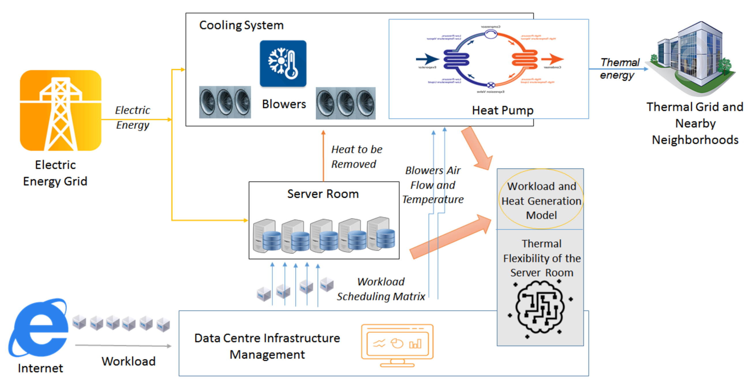
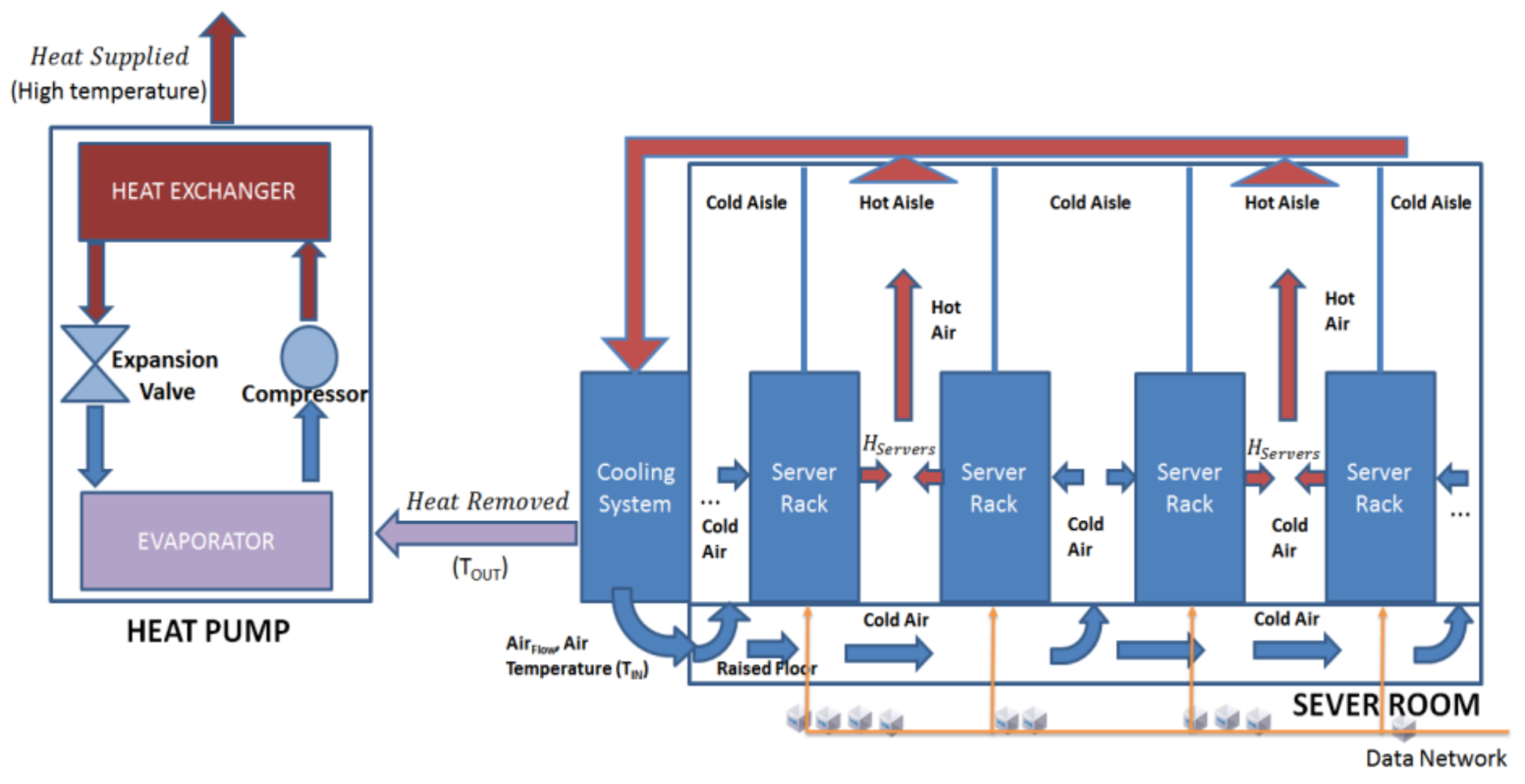
In this section, we introduce a mathematical model to relate the DC workload and associated electrical energy consumption with the generated thermal energy that must be dissipated by the cooling system (waste heat), as shown in Figure 1. The model’s objective is to provide the support necessary for the DC infrastructure management software in taking workload scheduling decisions as well as cooling system operation optimization decisions such that the DC thermal profile is adapted to meet the heat demand coming from nearby neighborhoods. The model is based on and enhances the previous one proposed by us in [45], this time focusing on the thermo-electrical model of the server room and energy dynamics by providing mathematical formalisms that relate the deployment of the VMs on the servers with the electrical energy consumption and thermal energy generation of the IT equipment. Furthermore, in this paper the relations between the IT equipment heat generation and cooling system thermal energy dissipation capabilities are presented, also considering the impact of the volume and temperature of the input airflow in the case of an air-cooled server room.

To execute the clients’ workload, the IT equipment from the server room consumes electrical energy which is transformed into heat that must be dissipated by the cooling system. If the DC is equipped with heat reuse technology, the heat pump can perform both cooling of the server room and waste heat reuse. We consider a cloud-based DC hosting applications for its clients in VMs. When the number of user requests for an application increases, the cloud platform load balancer automatically scales up or down the resources allocated to VMs. Thus, the workload is modeled as a set of VMs each having virtual resources allocated:

$$\{\begin{array}{c}Workload=\left\{V{M}_1,V{M}_2,\dots ,V{M}_M\right\}\\ V{M}_j=\left(CP{U}_j, RA{M}_j,HD{D}_j\right), 0\le j\le M\end{array}$$

(1)

The server room of the DC to be composed of set of N homogeneous servers defined according to relation (2) the main hardware resources of the server being the number of CPU cores, the RAM and the HDD capacity.

$$\{\begin{array}{c}Serve{r}_{Room}=\left\{Serve{r}_1,Serve{r}_2,\dots ,Serve{r}_N\right\}\\ Serve{r}_i=\left(CP{U}_i, RA{M}_i,HD{D}_i\right), 0\le i\le N\end{array}$$

(2)

We define an allocation matrix of the VMs on servers, $ϵR^{N \ast M}$, where the element $S\left[Serve{r}_i\right]\left[V{M}_j\right]$ is defined according to relation (3) and specifies if $V{M}_j$ is allocated to server $Serve{r}_i$:

$$S\left[Serve{r}_i\right]\left[V{M}_j\right]=\{\begin{array}{c}1, \mathrm{if} V{M}_j \mathrm{is} \mathrm{allocated} \mathrm{to} Serve{r}_i during time window T\\ 0, otherwise\end{array}$$

(3)

Using the S matrix, we can compute the utilization rate of server $Serve{r}_i$ over the time window of length T by summing the hardware resources used by the VMs allocated on this server. For example, in case of the CPU it is denoted as ${\mu }_{{server}_i}$, and calculated using the following relation:

$${\mu }_{{server}_i}=\frac{{{\displaystyle \sum }}_{j=1}^{M}S\left[i\right]\left[j\right]\times CP{U}_{{VM}_j}}{CP{U}_{{Server}_i}}$$

(4)

Knowing the utilization of the server, one can approximate the power consumed by the server using Equation (5) proposed in [3], that defines a linear relationship between the server utilization, the idle power consumption $P_{idle}$ and the maximum power consumption of the server $P_{max}$:

$$P_{server}\left({\mu }_{server}\right)=P_{idle}+{\mu }_{server}\times \left(P_{max}-P_{idle}\right)$$

(5)

The IT equipment energy demand over the time interval T can be computed as:

$$E_{IT}\left(T\right)={{\displaystyle \int }}_t^{t+T}{P}_{IT}\left(t\right)dt \mathrm{where}{P}_{IT}= {{\displaystyle \sum }}_{i=1}^n{P}_{server}\left({\mu }_{serve{r}_i}\right)$$

(6)

Most of the electrical energy consumed by the servers is converted to thermal energy that must be dissipated by the electrical cooling system for keeping the temperature in the server room below a defined set point:

$$Hea{t}_{Removed}\left(t\right)=E_{IT}\left(t\right)$$

(7)

The electrical cooling system is the largest energy consumer of the DC after the IT servers. Following our assumption of being equipped with heat reuse pumps, the cooling system must extract the excess heat from the server room and dissipate it into the atmosphere. By operating in this way there are two sources of energy losses: first the electrical energy needed to extract the heat from the server room and second the thermal energy dissipated. The main idea to increase efficiency is to use the heat pump to capture the excess heat and reuse it for nearby neighborhoods.

The heat pump operation is modeled leveraging two main parameters [8,24,25,26]: the COP for cooling, denoted as $CO{P}_{cooling}$ and the COP for heating, denoted as $CO{P}_{heating}$. The first parameter is calculated as the ratio between the heat absorbed by the heat pump, denoted $Hea{t}_{Removed}\left(t\right)$, and the work done by the compressor of the heat pump to transfer the thermal energy, in this case, represented by the electrical energy consumed by the heat pump compressor denoted as $E_{cooling}\left(t\right)$:

$$CO{P}_{cooling}=\frac{Hea{t}_{Removed}\left(t\right)}{E_{cooling}\left(t\right)}$$

(8)

The second parameter, the COP for heating, the relation between the heat produced by the heat pump and supplied in the nearby neighborhoods, $Hea{t}_{Suplied}\left(t\right)$, and the electrical energy consumed by the heat pump to extract the heat, $E_{cooling}\left(t\right)$.

$$CO{P}_{heating}=\frac{Hea{t}_{Supplied}\left(t\right)}{E_{cooling}\left(t\right)}+1$$

(9)

Using the thermodynamics law of heat capacity, the heat removed from the server room in a specific moment of time $t$ can be computed as the product between the airflow through the room, $ai{r}_{flow}\left(t\right)$, the specific heat of air, $c_{air}$, and the difference between the temperature of the air entering the room, $T_{IN}\left(t-dt\right)$, and exiting the room, $T_{OUT}\left(t\right)$, where $dt$ is the time needed by the air to pass through the room:

$$Hea{t}_{Removed}\left(t\right)=ai{r}_{flow}\left(t\right)\times c_{air}\times \left[T_{OUT}\left(t\right)-T_{IN}\left(t-dt\right)\right]$$

(10)

The air traveling through the server room takes the heat from the servers, increasing its temperature from $T_{IN}\left(t - dt\right)$ to $T_{OUT}\left(t\right)$ during a period $dt$. If during this interval, the heat removed by the air passing through the room is equal to the electrical energy consumed by the servers during this interval, then, according to relation (7) the temperature inside the room remains constant. Otherwise, the temperature inside the room can fluctuate, increasing or decreasing.

It is difficult to determine a relation between the input and output airflow temperature on one side and the server room temperature on the other side in different interest points because the thermodynamics of the room must be considered. Consequently, we have defined a function $T_{SIM}$ that takes as inputs the set of servers in the server room ($Serve{r}_{Room}$), the heat produced by each server, $H_{Serve{r}_i}$(considered equal to the energy consumed), the input airflow and temperature $T_{IN}, ai{r}_{flow}$ and computes the output temperature of the air leaving the room, $T_{OUT}$, and the temperatures in critical points of the server room, $T_{Serve{r}_i}^{Surround}$, after a time period $t$:

$$T_{SIM}\left(Serve{r}_{Room}, H_{Serve{r}_i}, T_{IN}, ai{r}_{flow},t\right)\to \left(T_{OUT}, T_{Serve{r}_i}^{Surround}\right)$$

(11)

For a given configuration of the DC and setting of the cooling system, the $T_{SIM}$ function computes the temperatures in the room after a time $t$. To function properly, the temperatures of the critical DC equipment must not exceed the manufacturer threshold:

$$T_{Serve{r}_i}^{Surround}<Threshol{d}_{Server}\forall i\in \left\{1 \dots N\right\}$$

(12)

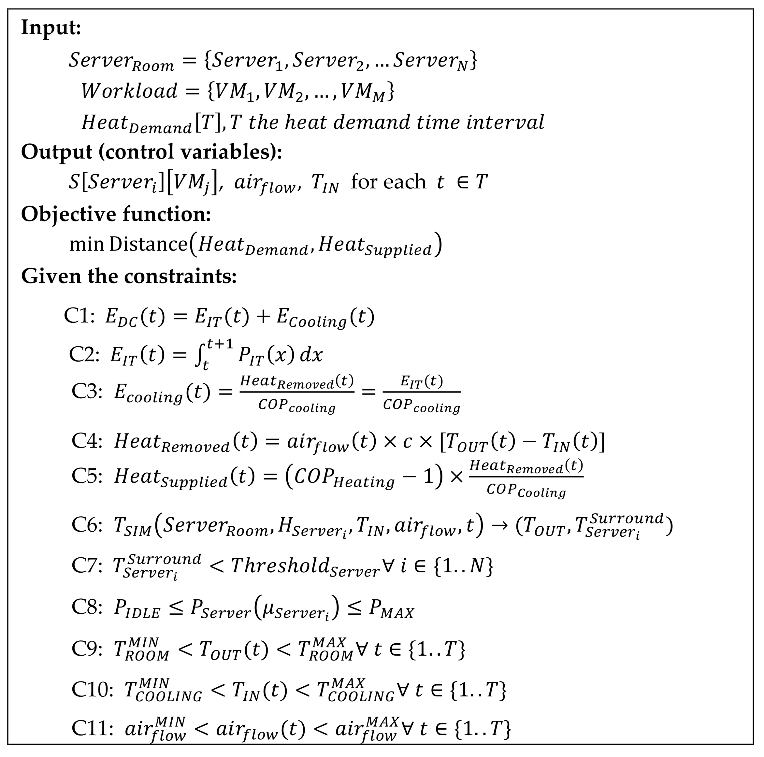
Because the aim of this paper is to define a proactive optimization methodology for DC waste heat reuse on-time window of length $T$, we choose to construct a discrete model of the thermodynamic processes described above and to split the time window $\left[0 \dots T\right]$ in $T$ equidistant time slots. Consequently, the values of the control variables of the cooling system equipped with heat reuse pumps as well as the workload allocation matrix will be computed. The optimization problem is defined in Figure 2.

The inputs are represented by the DC server room configuration, the workload that has to be deployed during and executed during the time window $\left[0 \dots T\right]$ as well as the heat demand profile $Hea{t}_{Demand}\left[T\right]$ (i.e., requested by the neighborhood) that has to be supplied $Hea{t}_{Supplied}$ by the DC computed using the model presented above. The outputs of the optimization problem are the scheduling matrix VMs to the servers, the airflow and air temperature of the cooling system for each time slot of the optimization window $\left[0 \dots T\right]$.

The defined optimization problem is a Mixed-Integer-Non-Linear Program (MINLP) [46] due to the nonlinearities of the objective function and the integer variables of the scheduling matrix. It can be shown that the resulting decision problem is NP-Hard [47], thus we have used a multi-gene genetic algorithm heuristic to solve the optimization problem, similar with the one presented by us [48]. The solution of the algorithm is represented by three chromosomes corresponding to the three unknowns of the optimization problem described in Figure 2. The chromosome corresponding to the $S$ workload scheduling matrix is an integer vector of size $M$, equal to the number of VMs. The chromosomes corresponding to the $ai{r}_{flow}$ and $T_{IN}$ variables are two real number arrays of length $T$, equal to the length of the optimization time window. As a result, we deal with a total number of $M$ integer and $2 \times T$ real unknowns. The fitness function is defined as the Euclidean distance between the heat profile of the DC corresponding to a solution and the heat demand. When evaluating each solution, the thermal profile of the DC is computed during the time window $\left[0 \dots T\right]$ by calling the $T_{SIM}$ function to compute the server temperatures. Thus, the run-time complexity of the genetic algorithm heuristic is:

$$O(N{o}_{iterations}\times Populatio{n}_{size}\times \left(T\times O\left(T_{SIM}\right)+T+M\right)$$

(13)

where $N{o}_{iterations}$ represents the number of iterations of the genetic a algorithm and $Populatio{n}_{size}$ the size of chromosomal population. The $T_{SIM}$ function implementation and time complexity is detailed in Section 4.

4. Thermal Flexibility of Server Room

An important component in adapting the DC thermal energy profile to meet a certain demand is the thermal energy flexibility of server room. Our objective is to estimate the available thermal energy flexibility considering different schedules of the workload to be executed and different settings of the cooling system (i.e., $T_{SIM}$ function behavior). This will allow us to obtain a high server utilization ratio and increase for limited time periods the temperature set points in the server room (i.e., allowing heat to accumulate) while being careful not to endanger the proper operation of IT equipment (i.e., servers’ temperature thresholds $T_{Serve{r}_i}^{Surround}$). Moreover, this will optimize the operation of the heat pump which will increase with more efficiency the temperature of waste heat leaving the server room, $T_{OUT}$, (i.e., due to higher temperature baseline) making the thermal energy more valuable and marketable.

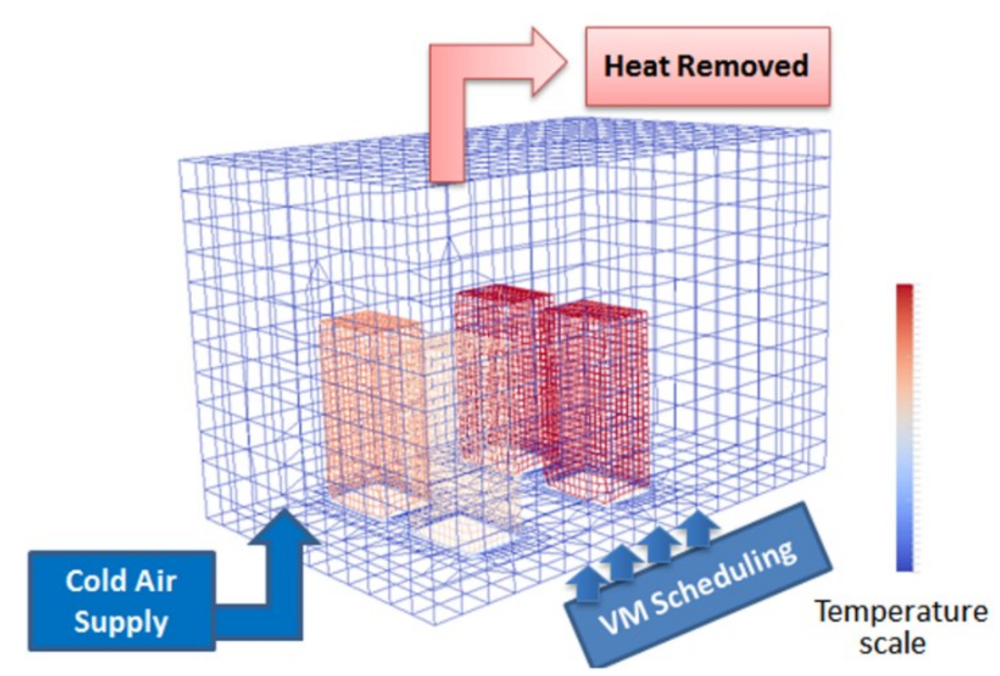
To estimate the thermal flexibility of the server room we have used CFD techniques to simulate the thermodynamic processes in the server room in relation to workload allocation on servers. We have considered a generic configuration of the server room as the one presented in Figure 3.

The server room is modeled as a parallelepiped with physical dimensions defined in tri-dimensional space expressed in meters (length, width, and height), number of homogenous blocks in which the server room volume will be divided, used for computing the simulation parameters, initial temperature at the beginning of the simulation, air substance characteristics and input airflow velocity vector and temperature. The solver will calculate the physical parameters of the simulation in each defined homogeneous block, the simulation accuracy depending on the size and number of these blocks. If they are smaller, the simulation is more accurate but takes longer to finish the calculations. Inside the server room, the server racks are defined as parallelepipeds with coordinates in tri-dimensional space having the reference frame the server room (X-coordinate, Y-coordinate, Z-coordinate), physical dimensions of each server rack expressed in meters (length, width and height), and average temperature of each rack due to server loads ($H_{Server}$).

Cold air is pumped in the room through raised floor perforated tiles and hot air is extracted through the ceiling. The heat reuse and cooling of the server room is performed using a heat pump similar to the solution presented in [9] featuring coefficients of performance for cooling and heating. The heat pump transfers the heat absorbed from the DC server room to the thermal grid by using a refrigerant-based cycle to increase its temperature and consuming electrical energy. The cooling system parameters are the input air velocity vector, defined as a vector in tri-dimensional space showing the direction and the speed of the air, the origin of the air velocity vector defined as a position in the server room space, and finally the temperature of the air supplied in the server room.

The control variables of the simulation are the two cooling system parameters (input airflow $ai{r}_{flow}$ and temperature $T_{IN}$) and the matrix of VMs scheduling on servers ($S$) from which the rack temperature is derived. From a thermodynamic point of view, the system operates as follows: cold air enters the cold aisle of the server room through the floor perforated tiles, passes through the racks, removing the heat generated by the electrical components. The hot air is eliminated behind the racks in the warm aisle. Due to its physical properties, the hot air rises, being absorbed by the ceiling fans and redirected to the main cooling unit containing cold water radiators that take over the heat from the air. The excess thermal energy from the air is passed to the water from the radiators that increases its temperature, while the air lowers its temperature and is pumped back to the room. The warm water is sent to the evaporator part of the heat pump that extracts the excess heat, lowering its temperature. The cold water is then pumped again back to the radiators, while the thermal energy extracted is transferred to the heat exchanger of the heat pump that heats water at the other end to temperatures as high as 80 degrees Celsius. Figure 4 presents the server room thermodynamic processes simulation view using OpenFoam [35].

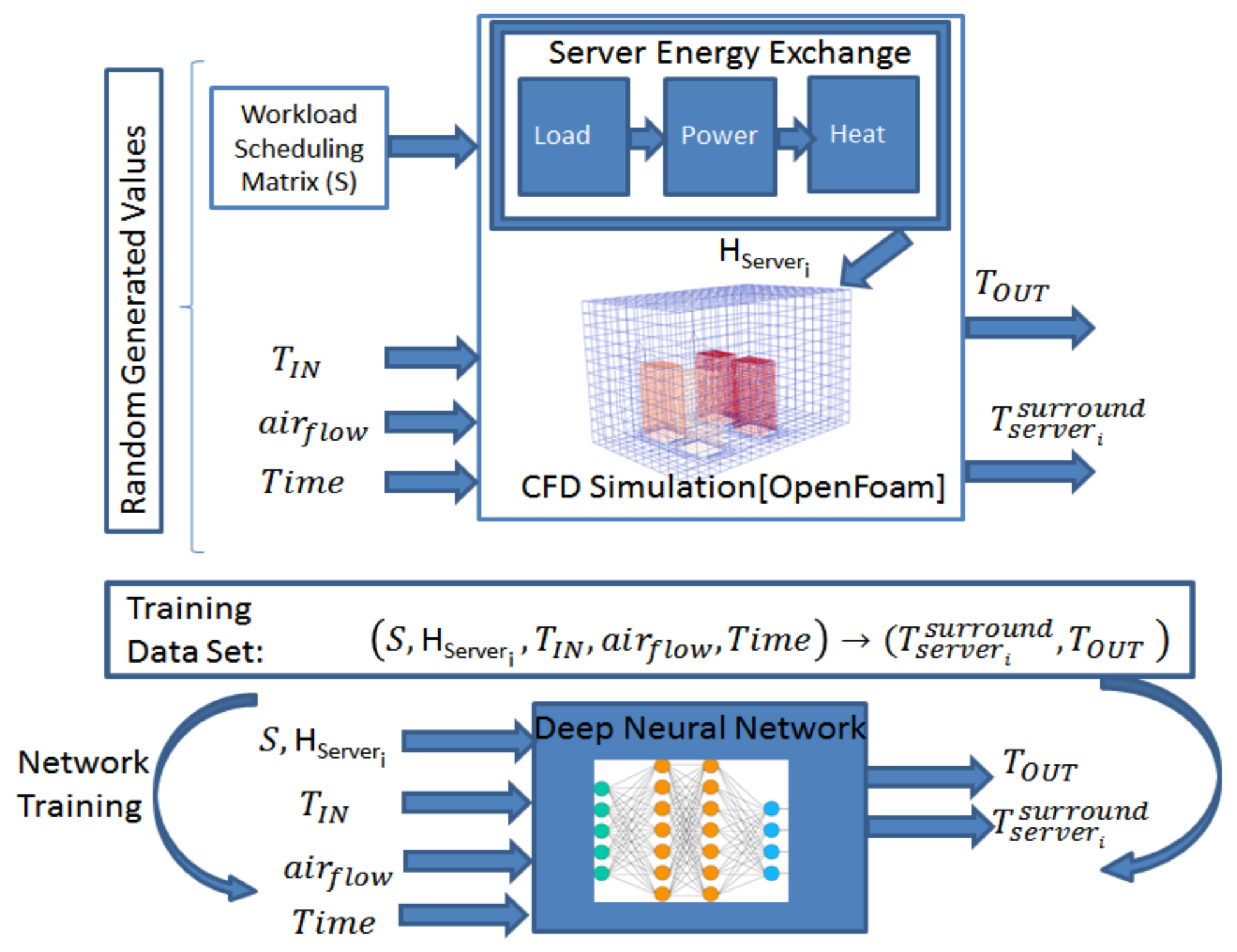
The advantage of using such a CFD-based simulation for determining the temperatures in the server room is the accuracy of the results, with the main drawback being the long execution time that makes it unsuitable for real-time iterative computations needed when solving the optimization problem described in Section 3. Thus, we have used deep neural networks-based technique to learn the $T_{SIM}$ function from a large number of samples, while using the OpenFoam CFD-based simulation to generate the training dataset (see Figure 5).

We have chosen the deep neural networks because they provide low time overhead during runtime (i.e., after training) and because the relations between the inputs and the outputs are non-linear and highly complex. The inputs of the neural network is represented by: (i) the matrix $S ϵR^{N \ast M}$ representing the VMs allocation on servers together with the array $H_{Serve{r}_i}$ representing the estimated heat generated by each of the N servers in the server room as result of executing the allocated workload; (ii) the airflow ($ai{r}_{flow}$) and temperature of the air fed ($T_{IN}$) into the room by the cooling system and (iii) the time interval for thermal flexibility estimation. From a structural point of view, the network used is a fully-connected one having $N + 3$ inputs and $N + 1$ outputs and two hidden layers. The neurons use Rectified Linear Unit (ReLU) activation functions and for training the network the ADAM optimizer [49] is used with the Mean-Square-Error (MSE) loss function.

The time complexity of the $T_{SIM}$ function is different in the two implementation cases. In the first case when CFD is used for implementation, the time complexity depends on the number of iterations of the simulation process and the complexity of an iteration. At its turn, the complexity of an iteration depends on several parameters, the most important being the accuracy of the surfaces modeled, while the number of iterations varies according to the convergence time of the model. In our implementation, a step of the simulation took about 1.5 s, and simulations converged in 100 up to 500 steps, so the simulation time could take up to 12 min. In the second case when neural networks have been used the complexity depends on the number of neurons of the network. However, the neural network call from Java environment was measured to be between 1 and 2 ms, with an average of 1.73 ms which represents a significant improvement in comparison to the CFD implementation.

5. Validation and Results

We have conducted numerical simulation-based experiments to estimate the potential of our techniques for exploiting the DCs thermal energy flexibility in reusing waste heat in nearby neighborhoods. The simulation environment is leveraging on a nonlinear programming solver to deal with the DC heat generation optimization as presented in Figure 2. For estimating the thermal flexibility of the server room the CFD-based techniques for simulating the thermodynamic processes involved were implemented using OpenFoam Open Source CFD Toolbox. It provides a set of C++ tools for developing numerical-based software simulations and utilities for solving continuous mechanics problems, including CFD related ones. Among the many solvers available in OpenFoam libraries we choose the BouyantBoussnesqSimpleFoam solver, which is suitable for heat transfer simulations and uncompressible stationary flow. The OpenFoam simulation process involves the following steps: (i) setting the parameters of the physical process underlying the simulation; (ii) setting the computational and space parameters of DC server room used in simulation and (iii) running the simulation and add the results to the neural network training data set. The neural network was implemented in Keras [50] with a Tensorflow [51] backend and was loaded in a Java application containing the solver for the optimization problem. For loading the network in Java, the Deeplearining4J framework [52] was used, that converts a JSON model of the network exported from Keras to the Java implementation.

In our experiments, we have modeled a DC server room of 6 m long, 4 m width and 4 m height, having a surface of 24 square meters and a volume of 96 cubic meters. The server room contains 4 standard 42U racks of servers (see

Table 1. Server Room Equipment Description.

Rack Type	Total Rack Idle Power [W]	Total Rack Max Power [W]	# Servers	Server Type	Server Idle Power [W]	Server Max Power [W]	# CPU Cores
HP Bladesystem C7000	2000	3000	10	IBM Blade	200	300	4
IBM Bladecenter S	4000	6000	20	IBM Blade	200	300	4
HP Bladesystem C7000	2550	4350	15	HP DL 360 G7	170	290	4
IBM Rack	5200	7200	20	IBM X3650 M4	260	360	4

) with the following dimensions: width −600 mm and depth-1000 mm, with both front and rear doors. The racks contain 10U Blade Systems servers with full-height and half-height blade servers featuring multiple power sources: 2U servers with 2 redundant power supplies or 1U servers with a single power supply.

The considered electrical cooling system (see

Table 2. Electrical cooling system characteristics.

Energy Consumption	Heat Generation	COPcooling	COPheating	Min Airflow	Max Airflow	Min TIN	Max TIN
5 kWh	7.5 kWh	3.8	2.3	~0.6 kg/s	~6 kg/s	14 °C	30 °C

) is based on indirect free cooling technology and consists on a set of redundant external chillers. Inside the server room, cooling is done by pumping cold air through the raised floor perforated to the server racks. The server racks are grouped in cool aisles, as shown in Figure 3.

The server racks are rear-to-back, being isolated from each other. Cold air enters a lane through the slopes of the floor, passes through the racks, taking over the heat of the electrical components. The hot air is discharged behind the racks in the warm corridor. Due to its physical properties, the hot air rises, being absorbed by the ceiling fans and redirected to the main cooling unit containing cold water radiators that take over the heat from the air as well as electric compressors used to cool the water. The heat reuse and cooling of the server room is performed using a heat pump having the characteristics presented in

Table 3. Heat exchange circuits characteristics.

Cooling System	Cooling Capacity (Operational Level)	24 kWh (Normal Operation)	4 kWh (Minimum)	48 kWh (Maximum)
Water Circuit	Water Flow	4120 L/h	687 L/h	8240 L/h
	Input Air Temperature	10 °C	10 °C	10 °C
	Output Air Temperature	15 °C	15 °C	15 °C
Air Circuit	Airflow	9340 m3/h	1600 m3/h	18,680 m3/h
	Input Air Temperature	17 °C	17 °C	17 °C
	Output Air Temperature	24 °C	24 °C	24 °C
	Air Mass	~3.18 kg/s	~0.6 kg/s	~6.5 kg/s

. There are two heat exchanges on the server room side of the cooling process: heat exchange between hot air extracted from the server room by the cooling system and cold water inside the radiators and heat exchange between cold air that is pumped into the room and IT servers to be cooled.

To train the neural network, a data set was generated by running 15,000 OpenFoam simulations considering different values of the input parameters such as workload scheduling matrix $S$, input airflow and temperature ($T_{IN}$ and $ai{r}_{flow}$). The simulation results were generated as tuples of the form $<Timestamp,<T_{OUT}, T_{rack-1},T_{rack-2},T_{rack-3},T_{rack-4}>>$, where $Timestamp$ is the simulation time instance when results are generated, $T_{OUT}$ represents output temperature of the air leaving the room, and $T_{rack-1},T_{rack-2},T_{rack-3},T_{rack-4}$ represent the surrounding temperatures of the 4 racks of server. Thus, a time log showing the progress of the server room temperatures is created containing more than 50,000 different data samples. The generated data set, together with the values of OpenFoam simulation input parameters is converted into a format accepted by the neural network, being split in 80% training data samples and 20% as test data samples for the neural network. When evaluating the precision of the temperature predictions using the trained neural network against a number of reference OpenFoam simulations we obtain the mean square error (MSE) and mean absolute percentage error (MAPE) values shown in

Table 4. Temperature Prediction based on Neural Network Model Evaluation.

Metric	${\mathit{T}}_{\mathit{o}\mathit{u}\mathit{t}}$	${\mathit{T}}_{\mathit{r}\mathit{a}\mathit{c}\mathit{k} - 1}$	${\mathit{T}}_{\mathit{r}\mathit{a}\mathit{c}\mathit{k} - 2}$	${\mathit{T}}_{\mathit{r}\mathit{a}\mathit{c}\mathit{k} - 3}$	${\mathit{T}}_{\mathit{r}\mathit{a}\mathit{c}\mathit{k} - 4}$	${\mathit{T}}_{\mathit{o}\mathit{u}\mathit{t}}$
MSE	0.19	2.21	0.08	0.53	0.11	0.11
MAPE	1.48%	3.26%	0.93%	2.26%	1.02%	1.05%

. They are computed using relations (14) and (15) where: $n$ is the number of samples considered, $Tem{p}_{Reference}$ is the reference temperature of one of the parameters generated from OpenFoam simulations (i.e., $T_{OUT}, T_{rack-1},T_{rack-2},T_{rack-3},T_{rack-4}$, etc.) and $Tem{p}_{Predicted}$ is the temperature predicted by our neural network model.

$$MSE=\frac{1}{n}\times {\displaystyle \sum }_{i=1}^n{\left(Tem{p}_{Reference}-Tem{p}_{Predicted}\right)}^2$$

(14)

$$\mathrm{MAPE}=\frac{100}{n}\times {\displaystyle \sum }_{i=1}^n\frac{\left|Tem{p}_{Reference}-Tem{p}_{Predicted}\right|}{Tem{p}_{Reference}}$$

(15)

The temperatures are measured on the Celsius scale and vary from 18 to 60 degrees, thus an error of 2% means a temperature miss prediction of about 1 degree Celsius. As it can be noticed from Table 4, the mean absolute error percentage of the predictions is less than 2% for the rack temperature prediction, meaning that the temperatures are predicted with an accuracy of 1 degree Celsius for the racks. The prediction error is the cost of cutting down the OpenFoam simulation time to less than 2 milliseconds needed to predict the temperatures using neural networks, being a reasonable tradeoff in case of DC optimization where multiple evaluations have to be carried out fast to determine an optimal parameter setting for DC operation.

5.1. Workload Scheduling and Temperature Set Points

This section evaluates the relation between the DC workload scheduling on servers ($S$ allocation matrix control variable defined in Section 3), heat generation in the server room and temperature set points. We aim to determine workload deployment strategies on servers which will allow us to maximize the average temperature in the server room without impacting the IT server operation through overheating (i.e., hot spots avoidance). To estimate the heat generated by the servers as result of workload execution we have used the relation between CPU (Central Processing Unit) usage and temperature presented in

Table 5. CPU Usage vs. Temperature.

Server Type	Processor Family	${\mathit{P}}_{\mathit{M}\mathit{A}\mathit{X}}$ [W]	Temperature vs. Power Relation	Typical Thermal Profile
IBM Blade	Intel Xeon E5-2600	135 W	$CP{U}_{Temp} =0.205$ *$CP{U}_{Power} +48.9$
HP DL 360 G7	Intel Xeon 5600	130 W	$CP{U}_{Temp} =0.190$ *$CP{U}_{Power} +55.7$
IBM X3650	Intel Xeon X5400	120 W	$CP{U}_{Temp} =0.221$ *$CP{U}_{Power} +43.5$

. The values are reported in the Processors Thermal Specifications sheets [53,54,55].

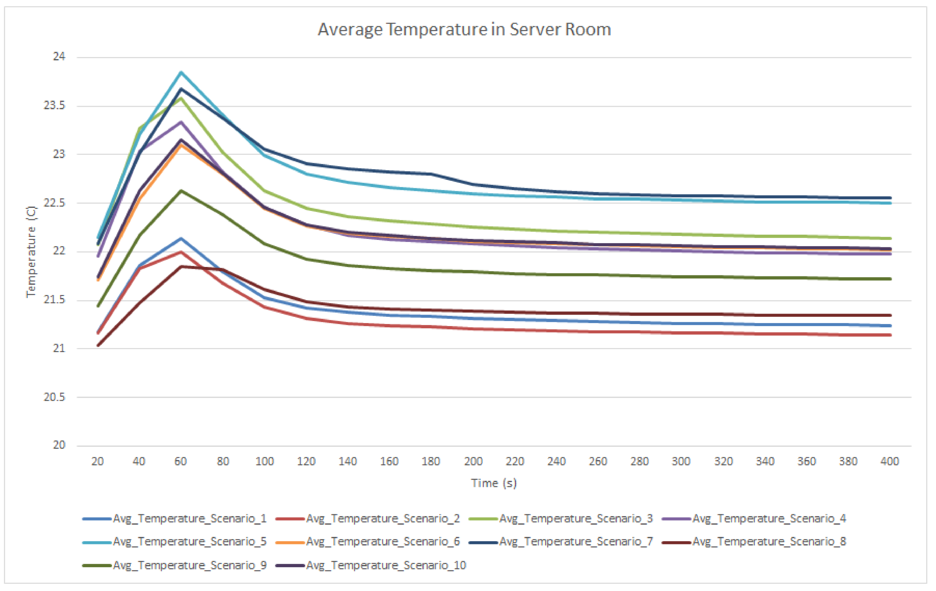
We have defined and used a set of 10 simulation scenarios. The cooling system is set to pump air in the room at a speed of 0.1 m/s and a volume of 3 kg/s at a temperature set point of 20 °C. The initial room temperature is also 20 °C. A set of 50 up to 65 synthetic VMs having 1 CPU core, 1 GB of RAM and 30 GB for HDD must be deployed in the virtualized environment running on the server racks. Each VM will run a synthetic workload that will keep its CPU between 80% and 100%.

Table 6. Workload Deployment in the DC and corresponding CPU usages.

Scenario	Rack 1		Rack 2		Rack 3		Rack 4		Total VMs Workload
	VMs	CPU Usage	VMs	CPU Usage	VMs	CPU Usage	VMs	CPU Usage
1	0	0	64	80	0	0	0	0	64
2	0	0	56	70	0	0	0	0	56
3	20	50	0	0	30	50	0	0	50
4	0	0	32	40	24	40	0	0	56
5	12	30	24	30	18	30	0	0	54
6	10	25	20	25	0	0	20	25	50
7	10	25	20	25	15	25	20	25	65
8	8	20	16	20	12	20	16	20	52
9	8	20	32	40	12	20	0	0	52
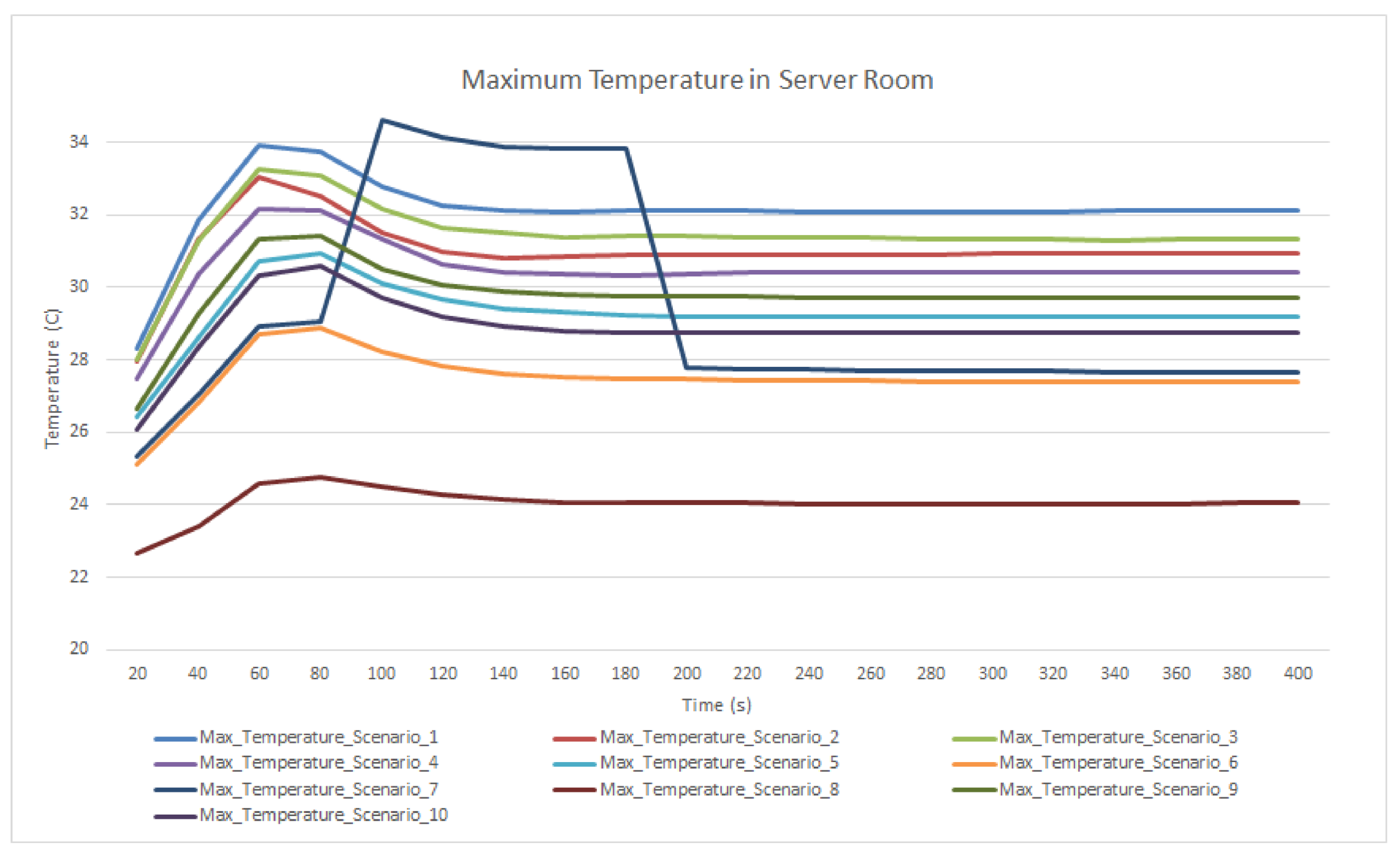
10	0	0	24	30	12	20	24	30	60

matrices of the VMs allocation on servers have been considered using two main workload scheduling strategies: either group the VMs on servers leading to an increased CPU usage (>50%) and increased CPU temperatures (Scenarios 1–3) or spread the VMs among more servers within each rack and have a lower CPU usage (<40%) and a lower CPU temperature (Scenarios 4–10). After simulating each workload scheduling configuration for 400 s, enough time to reach a thermal equilibrium for most scenarios, the average and maximum temperatures are plotted in Figure 6, respectively Figure 7.

As it can be seen from Figure 6, the highest average temperature in the server room is reached in the Scenarios 5–8, which disperse the workload among more servers with a lower utilization. The allocation technique that consolidates the workload on servers with high CPU usage, such as scenarios 1 and 2 show a smaller average temperature in the server room. Furthermore, by analyzing Figure 7 that displays the peak temperature in the server room, the situation is reversed. The deployment strategies in which the workload is consolidated on servers with high CPU usage exhibit the largest peak temperatures while the scenarios where the workload is spread on more servers with lower CPU usage show a lower maximum temperature in the server room. Even if at first sight these results are counter-intuitive, they can be explained. By distributing the workload on more servers with lower CPU usage, more thermal energy is released, because according to Equation (5) from Section 3, a server consumes electrical energy even in idle state, energy that will be converted in thermal energy which in turn will lead to a temperature increase in the server room. Thus, when the workload is consolidated on the minimum number of servers that run at high CPU usage, less electrical energy is consumed, and thus less thermal energy is eliminated in the room, a situation illustrated by a lower temperature in these scenarios. However, in these cases, because the energy is concentrated in a small number of points in the server room, hot spots might occur, as illustrated in Figure 7 by higher temperatures achieved by deployment strategies that overload the servers to use fewer resources.

In conclusion to transform the DCs in active thermal energy players which may provide heat in nearby neighborhoods the deployment strategies that maximize the average room temperature and minimize the maximum room temperatures are desired, for two reasons. Firstly, by having a higher average temperature in the server room, the exhaust air from the room is hotter and more heat can be recovered for heat reuse. Secondly, by minimizing the peak temperatures from the room, hotspots can be easily avoided in case of cooling system adjustments, such as pre- and post-cooling presented in the following section.

5.2. DC Thermal Profile Adaptation

This section aims at evaluating the DC capability of adapting its thermal energy generation to match a given heat demand by using only the cooling system control variables: input air temperature ($T_{IN}$) and input airflow ($ai{r}_{flow}$). By adjusting these two variables, the temperature in the server room can be increased for limited time periods allowing the DC to reuse the heat generating more efficiently through the heat pump and provide it to the nearby neighborhood. We have created four scenarios with a different combination of control variables adjustment (see

Table 7. Scenarios defined and control variables settings.

Scenarios	Heat Demand Matching (Before Optimization)	Control Variable		Heat Demand Matching (After Optimization)
		TIN	airflow
Post-cooling Scenario 1	63%	Constant at 20 °C	First decrease and then increase	98%
Post-cooling Scenario 2	79%	First increase and then decrease	Constant at 2.89 kg/s	97%
Pre-cooling Scenario 3	78%	Constant at 20 °C	First increase and then decrease	98%
Pre-cooling Scenario 4	86%	First decrease and then increase	Constant at 2.89 kg/s	99%

). For each of them we have evaluated the DC thermal flexibility over a period of two hours, with a five-minute time step, considering the same workload allocation matrix on servers (about 25% of the servers used).

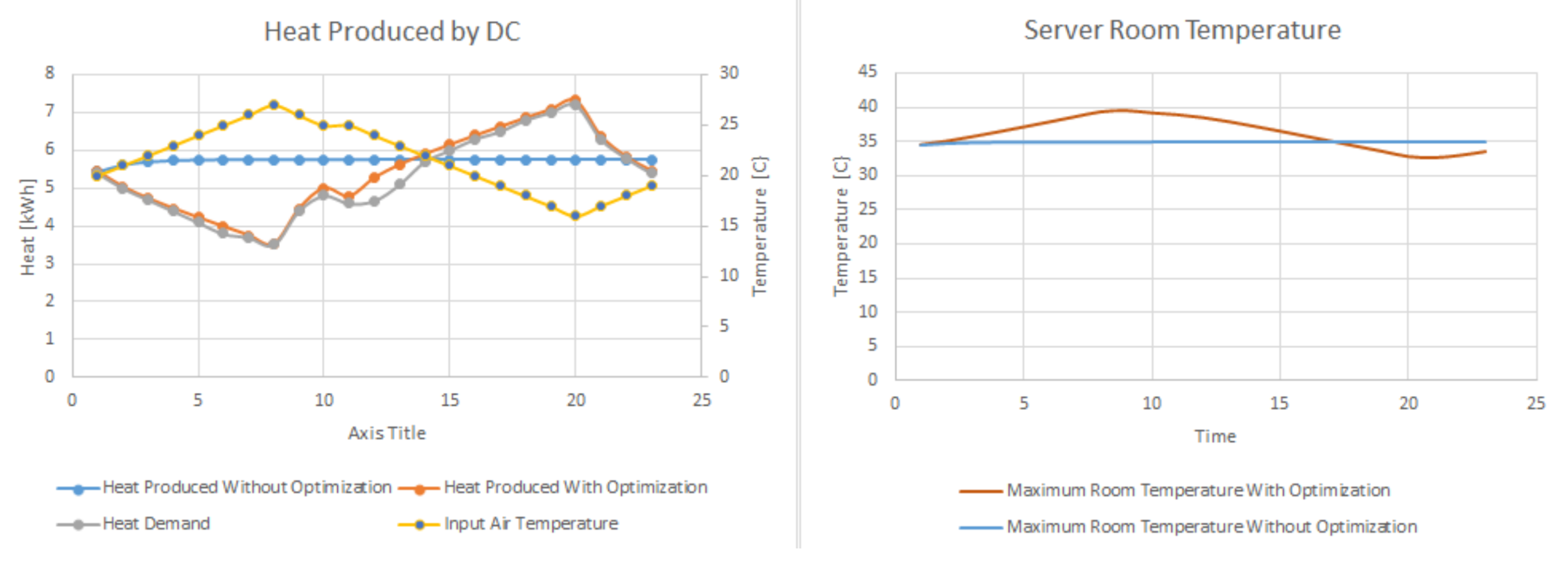
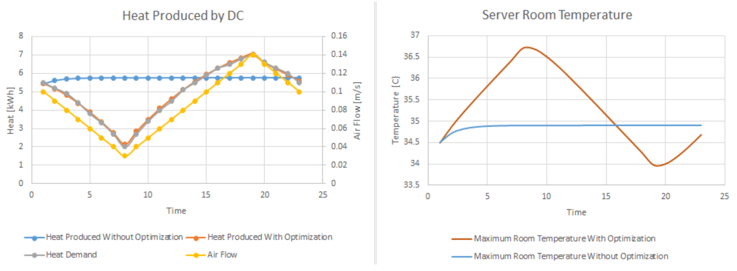
Scenarios 1 and 2 investigate the server room “post-cooling” mechanism as a source of thermal energy flexibility. In Scenario 1 the electrical cooling system usage is reduced for a short period of time to accumulate residual heat that can be later used to meet the heat demand. The cooling system input airflow ($ai{r}_{flow}$) is steadily decreased in the first 35 min, as shown by the yellow line in Figure 8-left, leading to an increase in the maximum temperature in the server room, as shown in Figure 8-right. Then, the airflow starts to steadily increase and to eliminate the excess residual heat from the server room, leading to a temperature decrease below the normal operating temperature shown by the blue line in Figure 8-right. Finally, in the last 15 min, the airflow is brought back to normal values leading to a rebalance of the server room operating temperature. By using this intelligent airflow management technique, the DC heat generation matches more than 98% the given heat demand profile.

In Scenario 2 we evaluate the DC thermal energy profile adaption by modifying the cooling system input air temperature ($T_{IN}$). Initially, the input airflow temperature is increased, as shown by the yellow line in Figure 9-left, a process that leads to an increase of the overall maximum server room temperature, is shown by the red line in Figure 9-right. The heat accumulates in the first hour in the server room. In the second hour, the input air temperature is steadily decreased below the normal operating set point temperature of 22 °C, shown by the blue line in Figure 9-left, increasing the amount of thermal energy removed from the server room. This thermal energy is transported to the heat pump that converts it to heat that can be reused to meet the nearby neighborhood heat demand profile with a matching degree of 97%.

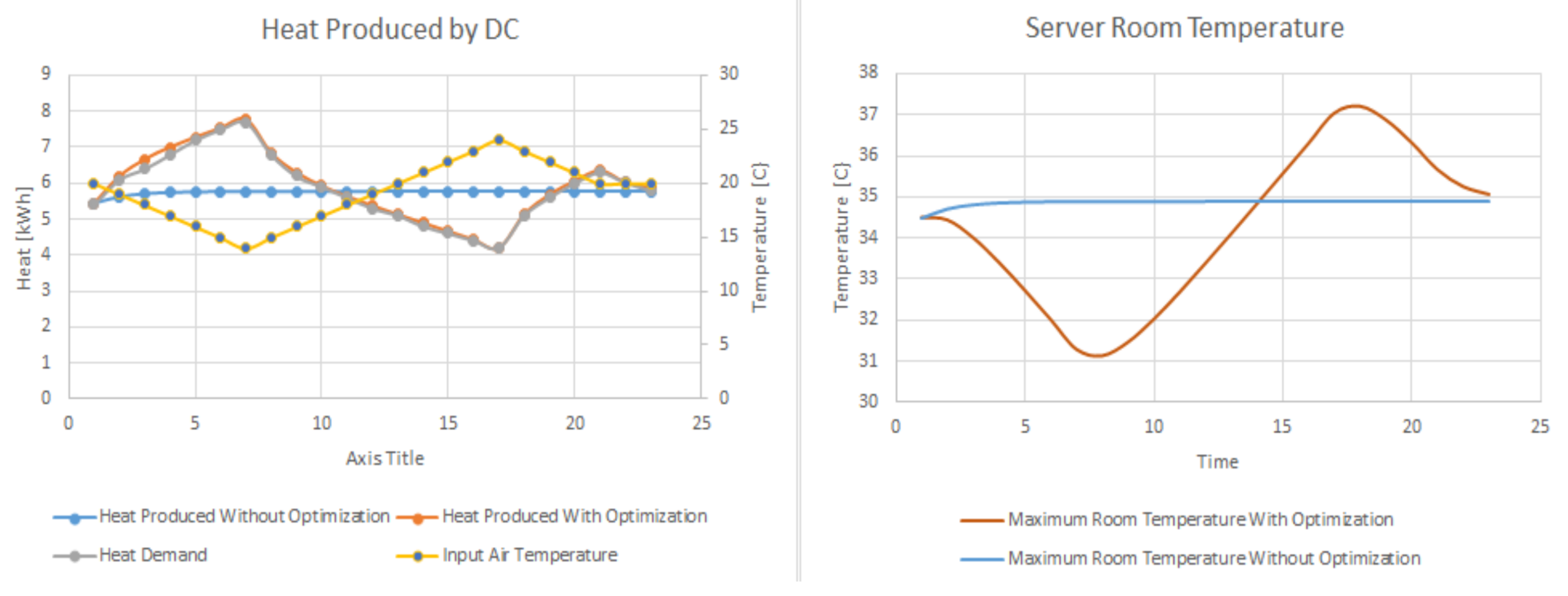
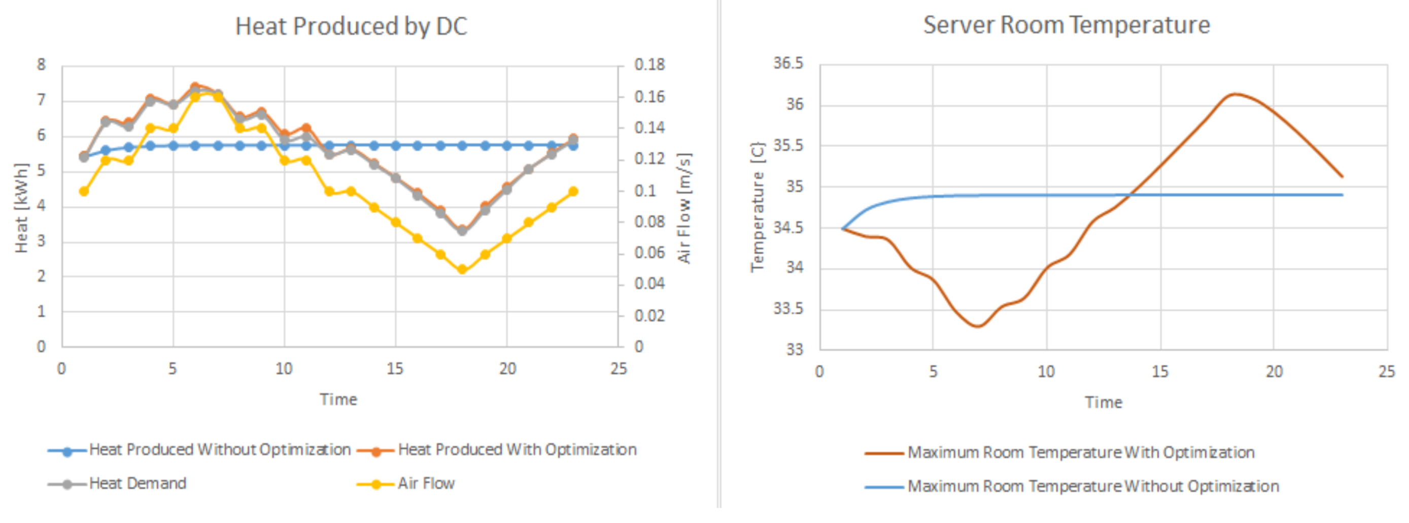
Scenarios 3 and 4 investigate the server room pre-cooling mechanism as a source of thermal energy flexibility. In scenario 3, as shown in Figure 10-left and Figure 10-right this is achieved toggling the airflow ($ai{r}_{flow}$) in the server room. To meet the increased heat demand of 7 kWh in the first 30 min of the simulation, the airflow is increased accordingly leading to an excess heat removal from the server room, as shown in Figure 10-right. Next, the heat demand is decreasing to 3 kWh, less than the normal 5.5 kWh heat generation of the servers. To meet this low heat demand, the cooling system airflow is drastically decreased, thus less heat is removed from the server room and the temperature increases. Finally, the airflow is brought back to normal values bringing back the temperature from the server room to the initial values. In this case, the heat demand is matched with an accuracy of 98%.

Scenario 4 presented in Figure 11 shows the DC response to an increased heat demand by adjusting the cooling system input air temperature ($T_{IN}$). In the first 30 min of the response period, the heat demand increases above 7 kWh, much higher than the 5.5 kWh normal thermal generation of the servers. To collect the necessary thermal energy, the cooling system decreases the input air temperature in the server room, removing more heat than generated, leading to a decrease in the server room temperature, as shown in Figure 11-right. In the second part of the response period, the heat demand decreases, thus the input air temperature is adjusted accordingly to remove less heat from the server room. As an impact, the average server room temperature increases and exceeds the normal operating temperature by 3°. In the last 15 min of the response, the DC adjust again the input air temperature to bring back the server room to normal operating parameters. In this case, the heat demand is matched with an accuracy of 99%.

6. Conclusions

In this paper, we have proposed techniques that will allow the DCs equipped with heat reuse technology to adapt their thermal energy profile and provide heat to nearby neighborhoods on demand. We have defined a mathematical model for describing the thermodynamics processes inside the server room and used it to decide on the optimal shifting DCs thermal energy profile to meet expected heat demands. CFD and neural networks have been employed to estimate the thermal flexibility of the DC considering the cooling system air temperature and flow level as control variables as well as workload allocation on servers to avoid hot spots. The validation conducted using the characteristics of a small DC was promising the results showing the DCs potential in acting as thermal energy players in their nearby neighborhoods. In our tests, the DC could meet the heat demand with an accuracy of over 90% in all the defined scenarios. As future work, we will investigate new business scenarios for DC operation which will allow them to cooperate and jointly exploit their thermal flexibility in providing a more stable heat supply and as result to gain new revenue streams. At the same time, we will address the case of fully decentralized DCs and supercomputers case which may provide free and efficient heating for residential buildings.