A Study on Green Supplier Selection in Dynamic Environment
by
 and
and
Wei Song
1, 
Zhiya Chen
2,
Aijun Liu
1,3,*,
Qiuyun Zhu
1,
Wei Zhao
1,
Sang-Bing Tsai
4,5,6,* and
Hui Lu
7 1
School of Economics and Management, Xidian University, No. 2 Taibai South Street, Xi’an 710071, China
2
School of Traffic and Transportation Engineering, Central South University, No. 932, Lushan South Road, Changsha 410083, China
3
State Key Laboratory for Manufacturing Systems Engineering, Xi’an Jiaotong University, Xi’an 710049, China
4
Zhongshan Institute, University of Electronic Science and Technology, Zhongshan 528400, China
5
Economics and Management College, Civil Aviation University of China, Tianjin 300300, China
6
Business and Law School, Foshan University, Foshan 528000, China
7
Tianhua College, Shanghai Normal University, Shanghai 201815, China
*
Authors to whom correspondence should be addressed.
Sustainability 2018, 10(4), 1226; https://doi.org/10.3390/su10041226
Submission received: 20 March 2018
/
Revised: 11 April 2018
/
Accepted: 12 April 2018
/
Published: 17 April 2018
(This article belongs to the Special Issue How does Outsourcing Affect the Economy and its Sustainability?)
Abstract
:The aim of this paper is to provide a method for selecting a green supplier in a dynamic environment, while considering the psychological behavior and the time factors of the decision maker from the manufacturer’s perspective. The supply selection method that is based on the Third Generation Prospect Theory (PT3) is proposed and an optimal ordinal number is obtained. First, the green supplier selection index system is established. Then, the indicators that are given by the manufacturer are used as reference points, and the income and loss matrices are established by calculating the gains and losses of the index values in the interval number relative to the reference points. Next, considering the time factor and calculating the variable weight based on the Gray correlation coefficient method and the time weight of the penalty mechanism method, the suppliers are chosen based on the comprehensive prospect value. Finally, the validity and the feasibility of the method are proven through a case analysis.
1. Introduction
With the acceleration of economic globalization, manufacturers face many challenges in terms of development and survival. An efficient supply chain management system can effectively improve the competitiveness of manufacturing enterprises, and supplier optimization is an important part of the supply chain management system. Therefore, supplier optimization has increasingly attracted attention, becoming a research hotspot for scholars, both nationally and globally. As the earth’s ecological environment worsens as the economy develops, the survival of humankind is being threatened. The development of a circular economy has become an important focus, and enterprises must be more socially responsible while continuing their own development. Manufacturing enterprises have also introduced the concept of “green” into supply chain management, and environmental performance is being gradually implemented as one of the evaluation standards to respond to the call of the public for more environmentally sustainable businesses. Green supplier selection plays a vital role in the green supply chain management. Selecting the most suitable supplier is the key for the success of a company. Companies could produce green products together with suppliers as a mutual cooperation relationship is developed [1,2]. With these relationships, companies could achieve the following: (1) reducing the number of to-be-delivered accessories with low environment performance; (2) effectively controlling the cost of suppliers’ green products; and, (3) decreasing the market response time. However, in the process of supplier optimization, complex problems are always simplified with heuristics. Through a large number of experiments, Kahneman and Tversky [3] proved that experience-based heuristics produce serious deviations, thus creating the prospect theory. The market environment is subject to constant dynamic changes in the process of supplier selection. To address the uncertainty in information and the environment, this paper proposes a third-generation prospect theory, the core of which addresses decision makers’ prospect value given constant change, with the state as the reference point, so that supplier selection is a dynamic and constantly changing process. However, the traditional supplier selection methods are static, and the impact of time on candidate enterprise evaluation results is rarely considered. Hence, in this paper, to create a more rational and scientific decision process, the possible circumstances in the supplier selection process are fully considered, and a penalty function is introduced into the process of solving the time weight.
The remainder of this paper is organized in the following manner. A literature review is provided in Section 2. The green supplier selection model is built based on third-generation prospect theory in Section 3. In Section 4, we establish the weight of indexes that is based on a generalized serial number, and then the comprehensive prospect value of each index is solved, In Section 5, an empirical example is provided to demonstrate the applicability of the proposed method. Section 6 provides a comparative analysis and discussion. Finally, some conclusions and relevant prospects are presented in Section 7.
2. Literature Review
Green supplier selection is a form of multi-objective decision making, which generally includes two parts: index selection and model construction. In terms of index selection, Lee et al. [4] improved the Delphi-Analytic Hierarchy Process (AHP) method by constructing a fuzzy analytic hierarchy evaluation model that is based on the Delphi method. By introducing innovative fuzzy set theory into the evaluation model, green supplier selection criteria in the new technology industry was studied. Then, the index system was introduced in the paper, which included six aspects: product quality, technical strength, pollution control, environment management quality, green products, and green technology. Awasthi et al. [5] proposed a method of evaluating supplier environmental performance based on fuzzy multi-criteria. Several of the most commonly used green supplier evaluation indexes were summarized from historical documents: clean material availability, environmental efficiency, green image, environmental costs, green products, environmental law, and green production management. Bai et al. [6] constructed a green supply chain evaluation method by using the grey system theory and rough sets, and summed the environmental metrics, including pollutant control, pollution prevention, the environmental management system, resource consumption, and the pollutant discharge ratio. Yu et al. [7] developed a fuzzy data envelopment analysis (FDEA) model to select the most suitable supplier. Production costs, lead time, and supply chain carbon footprints were used as the input criteria, and quality and demand quantity were used as the output criteria. Yeh et al. [8] designed a multi-objective genetic algorithm for green supplier selection, integrating four decision-making targets: cost, time, quality, and green rating. Green image, product recycling, green design, pollutant treatment cost, and environmental performance were considered as the supplier evaluation index. Yu et al. [9] proposed a carbon footprint-based incentive green supplier selection model. Both economic attributes (price, quantity, and lead time) and environmental attributes (green factors and carbon dioxide (CO2) emissions) were considered during the selection.
In terms of model construction, Chai et al. [10] argued that the most commonly used green supplier selection methods are the Analytic Hierarchy Process (AHP) and Technique for Order Preference by Similarity to an Ideal Solution (TOPSIS). AHP is an analytical method that divides complex decision-making systems into multiple levels. Tam et al. [11] used AHP to improve and optimize the decision-making process, and finally solved the problem of the long green supplier selection period that made it difficult for decision-makers to reach consensus given a conflict target. Handfield et al. [12] described the relative importance of AHP in green supplier selection when environmental factors were considered, illustrating the advantages and disadvantages of AHP and incorporating AHP into integrated information systems supporting environmental awareness procurement through three case studies. Kulak et al. [13] proposed a combination of multi-attribute axiomatic design (AD) and AHP, and compared the method to fuzzy AHP for the analysis of the method of setting the green supplier selection index. To maximize the corporate operation efficiency under multiple constraints, Mafakheri et al. [14] used AHP to evaluate suppliers. Shaw et al. [15] considered cost, defect rate, and delivery delay rate, using fuzzy AHP to analyze the weight of each index and applied it to fuzzy multi-objective linear programming. Finally, the effectiveness of the proposed method was proven.
TOPSIS is a comprehensive evaluation method that is used to judge the advantages and disadvantages of a scheme based on the distance and proximity between each method and the hypothetical optimal scheme. Boran et al. [16] proposed a green supplier selection method combining TOPSIS and intuitionistic fuzzy sets, in which the intuitionistic fuzzy weighted average operators were used to integrate decision makers’ views, and examples demonstrated the correctness of the intuitionistic fuzzy TOPSIS method. Given evaluation fuzziness and uncertainty, Wang et al. [17] proposed a fuzzy TOPSIS method to optimize the evaluation fuzziness and uncertainty in the process of green supplier selection, which greatly simplified the ideal distance solution. Liao et al. [18] integrated the fuzzy TOPSIS and multi-criteria decision method, which allowed for the manufacturer to set multiple rating levels for green supplier selection. Sharma et al. [19] proposed a three-stage model that was based on the Taguchi loss function, TOPSIS, and multi-criteria goal planning to help decision makers to choose superior suppliers. Dlalahet et al. [20] constructed a hybrid fuzzy model for multi-criteria decision making using an improved fuzzy Decision Making Trial and Evaluation Laboratory (DEMATEL) method to address the influence of the relationship between the evaluation criteria, and constructed an improved TOPSIS model for index evaluation of candidate suppliers. Given the fuzziness and subjectivity that is faced by a telecommunications company in an uncertain environment, Önüt et al. [21] constructed a model combining the analysis network process and ideal solutions (TOPSIS) using triangular fuzzy digital parametric language terminology. Iirajpour et al. [22] applied the approximate optimization solution method (TOPSIS) to the green supply chain selection process. Shenc et al. [23] used fuzzy set theory to improve the TOPSIS method; subjective human perception was transformed into real numbers by fuzzy set theory, and then the TOPSIS method was used to find the most suitable green suppliers for manufacturing enterprises.
In addition to the commonly used methods, since the relationship between green supplier selection indexes is unclear, Yang et al. [24] reported the subjective preferences of the evaluator using triangular fuzzy numbers, and proposed a fuzzy multi-criteria comprehensive decision-making method. Zhang et al. [25] studied the channel selection strategy of a corporation based on the agent-based modelling approach. They addressed the uncertainty that was derived from the heterogeneity of potential consumers’ valuations and schematically characterizing the demand distribution. Ishizaka [26] stated that an appropriate supplier selection method was critical for the success of a company. In this paper, the Fuzzy Analytic Hierarchy Process (FAHP) was used to identify a suitable supplier and its performance was demonstrated with a real-world case study for Toyota. For the uncertain, fuzzy, and dynamic information, such as unknown indices and weights, and for fuzzy semantics and dynamic time factors in green product collaboration design, Liu et al. [27] developed a two-stage dynamic hybrid Multi-Attribute Decision Making (MADM) approach to select design suppliers. Dou et al. [28] assessed green supplier development programs with a grey-analytical network process-based methodology under a grey fuzzy environment. Zhang and Xu [29] employed the qualitative flexible multiple (QUALIFLEX) method with a signed distance-based comparison method for selecting a green supplier under the hesitant fuzzy environment. Li et al. [30] proposed an extended qualitative flexible multiple (QUALIFLEX) method to solve problems regarding the selection of green suppliers using probability hesitant fuzzy information. Darabi and Heydari [31] used the fuzzy entropy method based on group decision analysis for green supplier selection under the interval-valued hesitant fuzzy environment. Awasthi and Kannan [32] discussed the green supplier development program using the nominal group technique and the vlsekriterijumska optimizacija I kompromisno resenje (VIKOR) method under fuzzy environment. Awasthi et al. [33] presented an integrated fuzzy AHP-VIKOR approach-based framework for sustainable global supplier selection. Mousakhani et al. [34] introduced a new model that was based on a group decision-making approach under novel compromise ranking method and interval type-2 fuzzy sets (IT2FSs) for the green supplier selection problems. Tsui et al. [35] integrated the preference ranking organization method for enrichment evaluations (PROMETHEE) and the influential network relation map (INRM) for enhancing the reliability of green supplier selection in the TFT-LCD industry. Büyüközkan and Çifçi [36] proposed a novel hybrid multi-criteria decision-making (MCDM) approach that was based on fuzzy DEMATEL, TOPSIS, and ANP to evaluate the green suppliers. When considering the uncertain returns from investments in supplier development, Mizgier et al. [37] proposed a multi-objective model for capital allocation for supplier development under risk. Carrera et al. [38] developed a fuzzy inference system that was suitable for all supply chain systems that can effectively solve the dynamic uncertainties in the green supplier selection process. Guo et al. [39] addressed the green supplier evaluation and selection problem in global apparel manufacturing by developing a methodological framework for green supplier evaluation and selection based on the triple bottom line principle and a fuzzy MCDM model. Choy et al. [40] proposed a green supplier selection method that was based on case-based reasoning neural network technology and intelligent supply chain management given subjective judgment and lack of systematic analysis in the green supplier selection process. Demirtas et al. [41] proposed a combination of Archimedes goal programming (AGP) and ANP with consideration for the multi-stage planning period of the green supplier selection process. In the green supplier selection process, Hsu et al. [42] optimized the fuzzy quality data and constructed the fuzzy index membership function of the candidate green supplier enterprise, laying a foundation for solving the nonlinear programming problem involving finite variables. Park and Lee [43] proposed a new comprehensive methodology for supplier selection. The approach is presented using an expectation maximization (EM) algorithm for clustering, data envelopment analysis (DEA) for efficiency, and analytic hierarchy process (AHP) for external function importance. Razmi et al. [44] proposed a nonlinear sub-model of ANP and mixed integers for supplier selection and order assignment.
From the above analysis, we can see that the traditional optimization methods, such as AHP, TOPSIS, DEMATEL, VIKOR, etc., have all been extended to green supplier selection problems. However, Green supplier selection belongs to a multi-attribute decision-making (MADM) problem, and the decision-makers’ psychological behavior and cultural factors will considerably impact the efficiency of supply chain coordination. Unfortunately, little attention has been paid to decision-makers’ psychological behavior analysis to handle multiple criteria green supplier selection. Therefore, fully considering the psychological behavior factors of the decision-maker is necessary. The prospect theory thus came into being as research progressed. Lahdelma et al. [45] proposed a new MADM method by combining prospect theory and the stochastic multi-attribute acceptable analysis method given stochastic MADM with incomplete preference information. Wang et al. [46] proposed a prospect scoring function-based interval intuitionistic fuzzy multi-attribute decision making method for MADM, with the attribute value as the interval intuitionistic fuzzy number. Grabisch et al. [47,48] considered the method where decision makers have two reference points for their attributes that are based on prospect theory. Because the above methods only consider the psychological behavior factors of the decision maker without considering time factors in the decision-making process, and research on green supplier optimization selection under this framework has not been completed, we propose a supplier selection method combining third-generation prospect theory and a generalized optimal ordinal number in a dynamic environment.
3. PT3-Based Green Supplier Selection Decision-Making Model
Supplier selection is influenced by the psychological behavior and time factors, which reflect the inherent imprecision and are difficult to describe accurately using simple language or mathematics. So, it can be said that supplier selection is a dynamic and fuzzy problem. The third-generation prospect theory takes decision makers’ constantly changing expectation as the reference point. For expression, fuzzy theory is more appropriate than probability theory to describe the psychological behavior of the decision makers [49,50]. Meanwhile, the interval number and the trapezoidal fuzzy number are needed to describe the evaluation indicators of candidate companies when the decision-makers have different acquaintances of the evaluation indicators. After the appropriate information conversion, the prospect decision matrix can be obtained by the third-generation prospect theory.
3.1. The Supplier Selection Evaluation Index System
During the development of a green supplier selection evaluation index, the psychological behavior factors of decision makers are fully considered, including risk, flexibility, and operability principles. The selected indexes not only correctly reflect the comprehensive ability of candidate enterprises, but they also allow for the manufacturers to modify, add, or delete the indexes according to their own situation. The survival of humankind is threatened as the world’s ecological environment is worsening as the economy develops. The development of a circular economy has become an area of interest, and enterprises must be more socially responsible while continuing their development. Manufacturing enterprises have introduced the concept of “green” into supply chain management, gradually using environmental performance as one of the evaluation standards to respond to the interest of the public. Therefore, for manufacturers’ to select optimal green suppliers, 10 evaluation indexes were screened in this paper, which are divided into cost and profitability indexes, as shown in Table 1.
3.2. Green Supplier Decision Model Based on the Third-Generation Prospect Theory
This paper presents a multi-attribute decision-making method that is based on the third-generation prospect theory (PT3) and generalized optimal ordinal number. This method sets the income matrix and the loss matrix, respectively, by calculating the gains and losses of the green supplier index value relative to the reference point, which is the expectation for the index that is given by the manufacturer. Then, the prospect decision matrix is established according to the PT3. For manufacturers, time is an important factor affecting enterprise competitiveness, and the importance of green suppliers varies with time. In this paper, the green supplier index values are quantified into a generalized optimal ordinal number, and a gray relational degree-based index weight calculation method and a timing weight determination method with a penalty mechanism are introduced based on the generalized optimal ordinal number for possible enterprise states in different time periods. Finally, comprehensive prospect values for each supplier are calculated and are sorted to select the optimal green supplier. A detailed description of the variables is provided in Table 2.
We assumed that the prospect is a clear number, and that the value can be one of three types of numbers: clear, interval, and trapezoidal fuzzy. The specific description for the three types of index values is as follows:
- (1)
- When the index , record , in which is a real number, . .
- (2)
- When the index , record , in which is an interval number, i.e., . In reality, the index value takes a random value from the interval in uniform distribution, with the probability density function as:
- (3)
- When the index , record , in which is the intuitive trapezoidal fuzzy number, that is, , , , , , , , , , , and its membership function is:where, is non-membership function. In general, in the intuitive trapezoidal fuzzy number , when , which can be recorded as . In this paper, we discuss fuzzy numbers of this type, and is the degree of hesitation. The smaller the value, the more determined the fuzzy number.
3.3. Calculation of Gains and Losses
First, we used the manufacturers’ expected value for the indexes as a reference point. Then, the gains and losses of each index were calculated relative to the reference point. When the index value was a clear number, the gain and loss values of the index were obtained, according to the calculation formula that is shown in Table A1 (Appendix A).
When the index value was an interval number, the calculation formula for each index value of the green supplier, according to the index value and the location of the reference point, is shown in Table A2 (Appendix A).
When the index value was an intuitive trapezoidal fuzzy number, the calculation formula for each index value of the green supplier, according to the index value and the location of the reference point, is shown in Table A3 (Appendix A).
3.4. Prospect Value Calculation and Scheme Sorting
Aiming at the income matrix and the risk loss matrix , the prospect value of each candidate’s index was calculated by considering the manufacturers’ different attitudes toward the risk of gains and losses. Here, the gain and loss value of each index for each supplier were first calculated. The value of gain , according to the prospect theory is:
The value of loss is:
where α and β represent the concave-convex degrees of gain and loss regions of the value function and , respectively, represents the manufacturer's degree of loss avoidance, λ > 1. Larger α and β indicate manufacturers’ higher acceptance of risk; a larger λ indicates a higher level of manufacturer loss avoidance. The probability weight of each green supplier’s gain and loss for each index was calculated separately. The formula for calculating the probability weight of gain is:
The formula for calculating the probability weight of loss is:
The selected parameter values were consistent with the experimental results [51,52]: , . Abdellaoui [53] and Xu [54] also experimentally studied the parameter values, and they obtained similar parameters.
We then calculated the prospect value of each green supplier for each index. The formula for calculating the prospect value of the green supplier for the index is:
According to Equation (7), the prospect decision matrix can be obtained as .
4. Weight Determination of Candidate Enterprises
To solve the challenge that is faced when the information about the cooperative enterprise is incomplete and the environment in which the manufacturer selects a green supplier is dynamic, we first transformed the data into the generalized optimal order matrix. Then, using gray correlation to calculate the weight of each index, the attenuation function of the penalty mechanism was introduced to determine the timing weight. Finally, we assembled the generalized optimal orderly number and the weight of all candidate green suppliers and chose the best candidate, according to the prospect value.
4.1. Generalized Optimal Ordinal Number
As shown by the variables in Table 2, represents the m green supplier enterprises providing services meeting the functional requirements; is the evaluation index consisting of n indexes; is the set of states of the candidate supplier enterprises in various periods, represents the index value of the green supplier for the ith index at time t, which can be either qualitative or quantitative, and allows for fuzziness and impossible comparison. It can be recorded as in the case of an impossible comparison, and can be expressed as in the form of a partial order or a preference structure in case the order of the index quality can only be obtained in the period where .
For the quantitative index, the value of each green supplier must be divided into n levels, and then the step length of index in a period can be expressed as:
Definition 1.
Let:
where is known as the generalized number of grade of index of green supplier at period t, superior to index of green supplier .
When , index of green supplier at period t is superior to index of green supplier by grades, which can be recorded as . When , it indicates that index of green supplier at period t is inferior to index of green suppler by grades, which can be recorded as . When , index of green supplier at period t is equal to the index of green supplier , which can be recorded as , and standardizing the decision matrix here is not needed.
Definition 2.
Let:
where ; when , . is known as the generalized optimal ordinal number of index of green supplier relative to index of supplier at period t.
Definition 3.
Let:
where represents the generalized optimal ordinal number of index of green supplier at period t; represents the generalized optimal ordinal number of green supplier at period t; and represents the generalized optimal ordinal number of . denotes the weight of Il at period t. represents the timing weight of the candidate green supplier.
4.2. Determine the Index Weight Based on the Correlation Coefficient Method
According to the generalized optimal ordinal matrix of index of green supplier at period t, the gray relational coefficient was used to solve the attribute weight. By using the gray correlation coefficient method for a comparative analysis of the data relationship of the system in different periods, the size of the green supplier index values was obtained.
where .
Calculate the average of the generalized optimal ordinal number of the green supplier index at period t:
where .
In each time period, select the generalized optimal ordinal number that is corresponding to the positive ideal scheme:
Calculate the deviation between the index of candidate green suppliers and at period t:
The gray relational coefficient of candidate green supplier regarding index and the positive ideal point at period t is:
where is generally 0.5 [52]. The weight of the attribute at period t can be expressed as:
4.3. Timing Weight Based on Penalty Mechanism
Due to the increasing complexity of the market environment, it is increasingly difficult for manufacturers to select optimal partners. Moreover, the supply chain management environment is dynamic and uncertain [54,55,56,57,58,59,60]. Due to the rapid development of each enterprise, a wide range of information is constantly changed, and older data are unlikely to correctly reflect green suppliers’ status quo. In this paper, a penalty function is introduced in order to better reflect candidate enterprises’ actual situation and to provide effective reference information for decision makers [61,62,63,64,65,66,67,68].
where represents the time attenuation factor that is used to control the attenuation speed and y − t represents the time interval between the observation period y and time period t. The weight of each time period is normalized to obtain the constant weight of each period as:
Assuming that each index is equally important to the manufacturing enterprise, then constant the weights of different indexes for the same time period are the same.
In this paper, a penalty function is introduced for individual enterprises to quickly improve the evaluation results, and an exponential variable weight method was used:
where indicates the degree of aversion for the candidate enterprise, indicates the penalty level. Enterprises with a generalized optimal ordinal number below will be penalized by increasing the time weight of the time period, and the timing weight of the candidate enterprise index is:
This weight reflects the time effectiveness, the dissatisfaction with unstable candidate enterprises, and candidate enterprises that are deliberately raising the evaluation results. The comprehensive prospect value is calculated for each supplier, according to the principle of simple weighting, and the formula is:
where .
According to the size of the comprehensive prospect value calculated based on Equation (22), the sorting result serves as an important basis for the manufacturer to select a supplier.
4.4. Supplier Selection Process Description
- Step 1: Develop the index system and index value of the reference point according to the enterprise development status.
- Step 2: Solve the corresponding gain and loss value according to the form and formula of each index value.
- Step 3: Convert the gain and loss value into a prospect decision matrix based on the gain and loss matrix and the corresponding probability weight.
- Step 4: Determine the weight of the generalized optimal ordinal number.
- Step 5: Determine the timing weight of the penalty mechanism.
- Step 6: Calculate the comprehensive prospect value of each candidate green supplier, according to the prospect decision matrix, the weight of the generalized optimal ordinal number, and the timing weight of the penalty mechanism.
- Step 7: Select the partner green supplier based on the comprehensive prospect value.
The specific process is shown in Figure 1.
5. Case Study
Automobile manufacturers are actively committed to independent, scientific, green, and harmonious enterprise development, and strive to create automotive companies that are more responsible and reliable. Given this context, we needed to choose a green supplier to cooperate and produce a batch of auto parts. Implementing the “the green value with green design, green supply, green manufacturing, and green marketing” concept improves the environmental protection management level of the supplier. The manufacturing company examined four suppliers, which were labeled as . The manufacturer comprehensively evaluated the four green suppliers according to the 10 indexes mentioned herein, with the evaluation indexes being recorded as , where represents the effectiveness index of cost index . According to laws in different development stages of enterprises and self-imposed conditions, Daft introduced the four main stages in organizational development: entrepreneurial, collectivization, standardization, and refinement. The probability of each stage is recorded as P = (0.3,0.3,0.2,0.2), according to the time span of each stage and the degree of importance of the production cost to each stage. The language variable is transformed into a clear number, interval number, or trapezoidal intuition fuzzy number, according to the actual index description language. The details are shown in Table 3.
The prospect value and each index weight of the candidate enterprise are displayed in Table 4.
When selecting a supplier, the decision maker’s evaluation of the candidate enterprise varies with time, and older evaluation results have lesser weight. In this paper, a penalty function was introduced with a timing variable weight method in order to prevent malicious and rapid improvement of comprehensive level by candidate enterprises. The penalty function is shown in Table 5.
According to the penalty function, timing weight of candidate enterprises for each index at each period is obtained in Table 6.
6. Discussion and Comparative Analysis
Based on the above calculation, the comprehensive prospect value of each candidate enterprise was obtained, as follows: . Based on the prospect theory, the suppliers were sorted according to the size of the comprehensive prospect value: . Hence, supplier is best for the manufacturer.
In this paper, a sensitivity analysis was completed for time attenuation factor that was involved in the time weight, which included the following cases: , , , and . The results are shown in Table 7.
The above results show that the value of the time attenuation factor does not exert an obvious effect on the comprehensive green supplier evaluation results, indicating the good stability of the evaluation results that are not affected by the personal preference of the decision makers. In addition, the proposed method was compared to the TOPSIS method and the variable weight dynamic multi-attribute method, which is commonly used for green supplier selection. The results of the comparison are shown in Table 8.
The evaluation results in Table 8 show slight differences in the sorting results of the three different methods to support decision makers in selecting the most appropriate supplier, which, however, do not affect the correctness of the manufacturer’s decision and demonstrate the effectiveness and the feasibility of the proposed method.
When compared to the other two methods, the outstanding advantages of the proposed approach in this study are as below: (1) The proposed method can measure the level of consistency in the judgments that are provided by a decision maker; (2) the proposed method easily completes an interchangeable conversion between qualitative concepts and quantitative information; (3) the proposed method can be used to optimize the green supplier selection problems where the weight information of criteria is completely unknown; and, (4) The proposed method can also capture uncertainty and vagueness of decision makers’ judgments because the verbal assessments are converted into crisp values. In addition, the method fully considers the psychological behavior and time factors.
7. Conclusions
Selecting a suitable supplier is one of the most important issues to achieve sustainable green management, which directly impacts the manufactures’ performance. From this perspective, the development and extension of a novel green supplier selection method is of substantial significance. Although many fuzzy MCDM methods have been applied to the green supplier selection problem, those methods can not consider the decision maker’s psychological behavior. Furthermore, they cannot solve the dynamics of the decision-making process. In this paper, the third-generation prospect theory and the generalized optimal ordinal number were combined to comprehensively evaluate green suppliers. It was demonstrated throughout the detailed calculation in the application that the proposed method is more efficient when compared with the methods of relevant studies. The following conclusions were drawn. (1) Green supplier selection is a multi-criteria decision problem. In this paper, decision-makers’ psychological behavior and possible circumstances in the decision-making process were fully considered and combined with a dynamic reference point in the third-generation prospect theory, so that the proposed method is more appropriate for the real green supplier selection process with greater plausibility. (2) Cooperation between manufacturers and green suppliers involves a long process. Therefore, we should fully consider the various factors. The proposed penalty function can prevent individual enterprises from maliciously improving their evaluation to help manufacturers make the best decisions. (3) In this paper, a sensitivity analysis was performed in order to evaluate the time attenuation factor. The result showed that variation in the attenuation factor does not affect the correct selection of the decision maker. The stability of the method based on the third-generation prospect theory and generalized optimal ordinal number in determining the candidate enterprises was proven. This study adds to the available methods and means for green supplier selection and better solves the actual decision-making issues in the fields of economy and management. (4) The manufacturing industry is a basic and important industry in our country. Choosing green suppliers can enhance the market competitiveness and protect the environment. Meanwhile, through the supplier selection method that is proposed in this study, good interactions between manufacturer and supplier can be increased to form closer cooperative relationships in the supply chain, which ultimately aids in the suppliers’ sustainable management and the creation of a win-win result. Therefore, studying supplier selection in green environments is essential. Furthermore, the study could be continued with anticipation that the proposed method could be used to resolve other similar supplier selection problems, such as product designer selection, sustainable supplier selection, and others.
Even with the advantages of the proposed approach, there are some limitations for further research. In the future research, it is worth integrating the PT3 method with other classical decision methods, such as TOPSIS, AHP, QFD, PROMETHEE, etc., and further considering the interaction among the criteria. In some situations, there are always various relationships among criteria. Therefore, the inter-dependent effects between evaluation criteria should be analyzed.
Acknowledgments
The study was supported by the “National Natural Science Foundation of China” (71401131), “MOE (Ministry of Education in China) Project of Humanities and Social Sciences” (13XJC630011), “Research Fund from Key Laboratory of computer integrated manufacturing in Guangdong Province” (CIMSOF2016002), “Central University Science Research Foundation of China” (JB170609), “China Postdoctoral Science Foundation funded project” (2016M590929), “the State Key Laboratory for Manufacturing Systems Engineering (Xi’an Jiaotong University, Xi’an, China)” (sklms2017005), “the Shaanxi Natural Science Foundation Project (2017JM7004) ” and the Zhongshan City Science and Technology Bureau Project (No. 2017B1015).
Author Contributions
This paper presents collaborative research results written by Wei Song, Zhiya Chen, Aijun Liu, Qiuyun Zhu, Wei Zhao. Wei Song and Zhiya Chen conceived and designed the study. Wei Song and Qiuyun Zhu performed the research and wrote the paper. Aijun Liu, Wei Zhao, Hui Lu, Sang-Bing Tsai checked English language and style. Sang-Bing Tsai provided revised advice. All authors read and approved the final manuscript.
Conflicts of Interest
The authors declare no conflict of interest.
Appendix A

Table A1.
The calculation formula when the index value is a clear number.
| Index Type | Relationship between the Expectation and the Reference Point | Calculation of the Gain and Loss Values (Gain Value ; Loss Value ) |
|---|---|---|
| (A1) (A2) | ||
| (A3) (A4) |
Table A2.
Calculation formula when the index value is an interval number.
| Index Type | Relationship between the Expectation and the Reference Point | Calculation of the Gain and Loss Value(Gain Value ; Loss Value ) |
|---|---|---|
| (A5) (A6) | ||
| (A7) (A8) | ||
| (A9) (A10) |
Table A3.
Calculation formula when the index value is intuitionistic fuzzy number.
| Index Type | Relationship between the Expectation and the Reference Point | Calculation of the Gain and Loss Value (Gain Value ; Loss Value ) |
|---|---|---|
| (A11) (A12) | ||
| (A13) (A14) | ||
| (A15) (A16) |
References
- Noci, G. Designing ‘green’ vendor rating systems for the assessment of a supplier’s environmental performance. Eur. J. Purch. Supply Manag. 1997, 3, 103–114. [Google Scholar] [CrossRef]
- Liu, A.J.; Hu, H.S.; Zhang, X.; Lei, D.M. Novel Two-Phase Approach for Process Optimization of Customer Collaborative Design Based on Fuzzy-QFD and DSM. IEEE Trans. Eng. Manag. 2017, 64, 193–207. [Google Scholar] [CrossRef]
- Kahneman, D.; Tversky, A. Prospect Theory: An Analysis of Decision under Risk. Econometrica 1979, 47, 263–291. [Google Scholar] [CrossRef]
- Lee, A.H.I.; Kang, H.Y.; Hsu, C.F.; Hung, H.-C. A green supplier selection model for high-tech industry. Expert Syst. Appl. 2009, 36, 7917–7927. [Google Scholar] [CrossRef]
- Awasthi, A.; Chauhan, S.S.; Goyal, S.K. A fuzzy multi criteria approach for evaluating environmental performance of suppliers. Int. J. Prod. Econ. 2010, 126, 370–378. [Google Scholar] [CrossRef]
- Bai, C.; Sarkis, J. Green supplier development: Analytical evaluation using rough set theory. J. Clean. Prod. 2010, 18, 1200–1210. [Google Scholar] [CrossRef]
- Yu, M.C. Using Fuzzy DEA for Green Suppliers Selection Considering Carbon Footprints. Sustainability 2017, 9, 495. [Google Scholar] [CrossRef]
- Yeh, W.C.; Chuang, M.C. Using multi objective genetic algorithm for partner selection in green supply chain problems. Expert Syst. Appl. 2011, 38, 4244–4253. [Google Scholar] [CrossRef]
- Yu, F.; Yang, Y.; Chang, D.; Yu, F.; Yang, Y.; Chang, D. Carbon footprint based green supplier selection under dynamic environment. J. Clean. Prod. 2018, 170, 880–889. [Google Scholar] [CrossRef]
- Chai, J.; Liu, J.N.K.; Ngai, E.W.T. Application of decision-making techniques in supplier selection: A systematic review of literature. Expert Syst. Appl. 2013, 40, 3872–3885. [Google Scholar] [CrossRef]
- Tam, M.C.Y.; Tummala, V.M.R. An application of the AHP in vendor selection of a telecommunications system. Omega 2001, 29, 171–182. [Google Scholar] [CrossRef]
- Handfield, R.; Walton, S.V.; Sroufe, R.; Melnyk, S.A. Applying environmental criteria to supplier assessment: A study in the application of the Analytical Hierarchy Process. Eur. J. Oper. Res. 2002, 141, 70–87. [Google Scholar] [CrossRef]
- Kulak, O.; Kahraman, C. Fuzzy multi-attribute selection among transportation companies using axiomatic design and analytic hierarchy process. Inf. Sci. 2005, 170, 191–210. [Google Scholar] [CrossRef]
- Mafakheri, F.; Breton, M.; Ghoniem, A. Supplier selection-order allocation: A two-stage multiple criteria dynamic programming approach. Int. J. Prod. Econ. 2011, 132, 52–57. [Google Scholar] [CrossRef]
- Shaw, K.; Shankar, R.; Yadav, S.S.; Thakur, L.S. Supplier selection using fuzzy AHP and fuzzy multi-objective linear programming for developing low carbon supply chain. Expert Syst. Appl. 2012, 39, 8182–8192. [Google Scholar] [CrossRef]
- Boran, F.E.; Genç, S.; Kurt, M.; Akay, D. A multi-criteria intuitionistic fuzzy group decision making for supplier selection with TOPSIS method. Expert Syst. Appl. 2009, 36, 11363–11368. [Google Scholar] [CrossRef]
- Wang, J.W.; Cheng, C.H.; Huang, K.C. Fuzzy hierarchical TOPSIS for supplier selection. Appl. Soft Comput. 2009, 9, 377–386. [Google Scholar] [CrossRef]
- Liao, C.N.; Kao, H.P. An integrated fuzzy TOPSIS and MCGP approach to supplier selection in supply chain management. Expert Syst. Appl. 2011, 38, 10803–10811. [Google Scholar] [CrossRef]
- Sharma, S.; Balan, S. An integrative supplier selection model using Taguchi loss function, TOPSIS and multi criteria goal programming. J. Intell. Manuf. 2013, 24, 1123–1130. [Google Scholar] [CrossRef]
- Dalalah, D.; Hayajneh, M.; Batieha, F. A fuzzy multi-criteria decision making model for supplier selection. Expert Syst. Appl. 2011, 38, 8384–8391. [Google Scholar] [CrossRef]
- Önüt, S.; Kara, S.S.; Işik, E. Long term supplier selection using a combined fuzzy MCDM approach: A case study for a telecommunication company. Expert Syst. Appl. 2009, 36, 3887–3895. [Google Scholar] [CrossRef]
- Iirajpour, A.; Hajimirza, M.; Najafabadi, A.F.; Kazemi, S. Identification and ranking of factors effective on performance of green supply chain suppliers: Case study: Iran Khodro Industrial Group. J. Basic Appl. Sci. Res. 2012, 2, 4633–4638. [Google Scholar]
- Shen, L.; Olfat, L.; Govindan, K.; Khodaverdi, R.; Diabat, A. A fuzzy multi criteria approach for evaluating green supplier’s performance in green supply chain with linguistic preferences. Resour. Conserv. Recycl. 2013, 74, 170–179. [Google Scholar] [CrossRef]
- Yang, J.L.; Chiu, H.N.; Tzeng, G.H.; Yeh, R.H. Vendor selection by integrated fuzzy MCDM techniques with independent and interdependent relationships. Inf. Sci. 2008, 178, 4166–4183. [Google Scholar] [CrossRef]
- Zhang, W.G.; Zhang, Q.; Mizgier, K.J.; Zhang, Y. Integrating the customers’ perceived risks and benefits into the triple-channel retailing. Int. J. Prod. Res. 2017, 55, 6676–6690. [Google Scholar] [CrossRef]
- Ishizaka, A. Comparison of fuzzy logic, AHP, FAHP and hybrid fuzzy AHP for new supplier selection and its performance analysis. Int. J. Integr. Supply Manag. 2014, 9, 1–22. [Google Scholar] [CrossRef] [Green Version]
- Liu, A.; Liu, H.; Xiao, Y.; Tsai, S.-B.; Lu, H. An Empirical Study on Design Partner Selection in Green Product Collaboration Design. Sustainability 2018, 10, 133. [Google Scholar] [CrossRef]
- Dou, Y.; Zhu, Q.; Sarkis, J. Evaluating green supplier development programs with a grey-analytical network process-based methodology. Eur. J. Oper. Res. 2014, 233, 420–431. [Google Scholar] [CrossRef]
- Zhang, X.; Xu, Z. Hesitant fuzzy QUALIFLEX approach with a signed distance-based comparison method for multiple criteria decision analysis. Expert Syst. Appl. 2015, 42, 873–884. [Google Scholar] [CrossRef]
- Li, J.; Wang, J.Q. An Extended QUALIFLEX Method under Probability Hesitant Fuzzy Environment for Selecting Green Suppliers. Int. J. Fuzzy Syst. 2017, 19, 1866–1879. [Google Scholar] [CrossRef]
- Darabi, S.; Heydari, J. An Interval-Valued Hesitant Fuzzy Ranking Method based on Group Decision Analysis for Green Supplier Selection. IFAC-PapersOnLine 2016, 49, 12–17. [Google Scholar] [CrossRef]
- Awasthi, A.; Kannan, G. Green supplier development program selection using NGT and VIKOR under fuzzy environment. Comput. Ind. Eng. 2016, 91, 100–108. [Google Scholar] [CrossRef]
- Awasthi, A.; Govindan, K.; Gold, S. Multi-tier sustainable global supplier selection using a fuzzy AHP-VIKOR based approach. Int. J. Prod. Econ. 2018, 195, 106–117. [Google Scholar] [CrossRef]
- Mousakhani, S.; Nazari-Shirkouhi, S.; Bozorgi-Amiri, A. A Novel Interval Type-2 Fuzzy Evaluation Model based Group Decision Analysis for Green Supplier Selection Problems: A Case Study of Battery Industry. J. Clean. Prod. 2017, 168, 205–218. [Google Scholar] [CrossRef]
- Tsui, C.-W.; Tzeng, G.-H.; Wen, U.-P. A hybrid MCDM approach for improving the performance of green suppliers in the TFT-LCD industry. Int. J. Prod. Res. 2015, 53, 6436–6454. [Google Scholar] [CrossRef]
- Büyüközkan, G.; Çifçi, G. A novel hybrid MCDM approach based on fuzzy DEMATEL, fuzzy ANP and fuzzy TOPSIS to evaluate green suppliers. Expert Syst. Appl. 2012, 39, 3000–3011. [Google Scholar] [CrossRef]
- Mizgier, K.J.; Pasia, J.M.; Talluri, S. Multiobjective capital allocation for supplier development under risk. Int. J. Prod. Res. 2017, 55, 5243–5258. [Google Scholar] [CrossRef]
- Carrera, D.A.; Mayorga, R.V. Supply chain management: A modular Fuzzy Inference System approach in supplier selection for new product development. J. Intell. Manuf. 2008, 19, 1–12. [Google Scholar] [CrossRef]
- Guo, Z.; Liu, H.; Zhang, D.; Yang, J. Green supplier evaluation and selection in apparel manufacturing using a fuzzy multi-criteria decision-making approach. Sustainability 2017, 9, 650. [Google Scholar]
- Choy, K.L.; Lee, W.B.; Lo, V. An intelligent supplier management tool for benchmarking suppliers in outsources manufacturing. Expert Syst. Appl. 2002, 22, 213–224. [Google Scholar] [CrossRef]
- Demirtas, E.A.; Ustun, O. Analytic network process and multi-period goal programming integration in purchasing decisions. Comput. Ind. Eng. 2009, 56, 677–690. [Google Scholar] [CrossRef]
- Hsu, B.M.; Chiang, C.Y.; Shu, M.H. Supplier selection using fuzzy quality data and their applications to touch screen. Expert Syst. Appl. 2010, 37, 6192–6200. [Google Scholar] [CrossRef]
- Park, S.C.; Lee, J.H. Supplier selection and stepwise benchmarking: A new hybrid model using DEA and AHP based on cluster analysis. J. Oper. Res. Soc. 2018, 69, 449–466. [Google Scholar] [CrossRef]
- Razmi, J.; Rafiei, H. An integrated analytic network process with mixed-integer non-linear programming to supplier selection and order allocation. Int. J. Adv. Manuf. Technol. 2010, 49, 1195–1208. [Google Scholar] [CrossRef]
- Lahdelma, R.; Salminen, P. SMAA-2: Stochastic Multicriteria Acceptability Analysis for Group Decision Making. Oper Res. 2001, 49, 444–454. [Google Scholar] [CrossRef]
- Wang, Z.; Li, K.W.; Wang, W. An approach to multiattribute decision making with interval-valued intuitionistic fuzzy assessments and incomplete weights. Inf. Sci. 2009, 179, 3026–3040. [Google Scholar] [CrossRef]
- Grabisch, M.; Labreuche, C.; Vansnick, J.C. On the extension of pseudo-Boolean functions for the aggregation of interacting criteria. Eur. J. Oper. Res. 2003, 148, 28–47. [Google Scholar] [CrossRef]
- Grabisch, M.; Greco, S.; Pirlot, M. Bipolar and bivariate models in multicriteria decision analysis: Descriptive and constructive approaches. Int. J. Intell. Syst. 2008, 23, 930–969. [Google Scholar] [CrossRef] [Green Version]
- Lawry, J. Probability, fuzziness and borderline cases. Int. J. Approx. Reason. 2014, 55, 1164–1184. [Google Scholar] [CrossRef]
- Singpurwalla, N.D.; Booker, J.M.; Lindley, D.V.; Laviolette, M.; Zadeh, L.A.; Dempster, A.P. Membership Functions and Probability Measures of Fuzzy Sets [with Comments, Rejoinder]. Publ. Am. Stat. Assoc. 2004, 99, 867–877. [Google Scholar] [CrossRef]
- Chu, T.C.; Varma, R. Evaluating suppliers via a multiple levels multiple criteria decision making method under fuzzy environment. Comput. Ind. Eng. 2012, 62, 653–660. [Google Scholar] [CrossRef]
- Tversky, A.; Kahneman, D. Advances in prospect theory: Cumulative representation of uncertainty. J. Risk Uncedtain. 1992, 5, 297–323. [Google Scholar] [CrossRef]
- Abdellaoui, M. Parameter-free elicitation of utility and probability weighting functions. Manag. Sci. 2000, 46, 1497–1512. [Google Scholar] [CrossRef]
- Tsai, S.-B.; Wei, Y.-M.; Chen, K.-Y.; Xu, L.; Du, P.; Lee, H.-C. Evaluating Green Suppliers from Green Environmental Perspective. Environ. Plan. B Plan. Des. 2016, 43, 941–959. [Google Scholar] [CrossRef]
- Lee, Y.C.; Wang, Y.-C.; Lu, S.-C.; Hsieh, Y.-F.; Chien, C.-H.; Tsai, S.-B.; Dong, W. An empirical research on customer satisfaction study: A consideration of different levels of performance. Springerplus 2016, 5, 1577. [Google Scholar] [CrossRef] [PubMed]
- Wang, J.; Yang, J.; Chen, Q.; Tsai, S.-B. Creating the sustainable conditions for knowledge information sharing in virtual community. Springerplus 2016, 5, 1019. [Google Scholar] [CrossRef] [PubMed]
- Tsai, S.-B. Using the DEMATEL model to explore the job satisfaction of research and development professionals in China’s photovoltaic cell industry. Renew. Sustain. Energy Rev. 2018, 81, 62–68. [Google Scholar] [CrossRef]
- Lee, Y.-C.; Hsiao, Y.-C.; Peng, C.-F.; Tsai, S.-B.; Wu, C.-H.; Chen, Q. Using Mahalanobis–Taguchi system, logistic regression, and neural network method to evaluate purchasing audit quality. Proc. IMechE Part B J. Eng. Manuf. 2014. [Google Scholar] [CrossRef]
- Liu, B.; Li, T.; Tsai, S.-B. Low carbon strategy analysis of competing supply chains with different power structures. Sustainability 2017, 9, 835. [Google Scholar] [CrossRef]
- Huang, Z.; Nie, J.; Tsai, S.-B. Dynamic Collection Strategy and Coordination of a Remanufacturing Closed-Loop Supply Chain under Uncertainty. Sustainability 2017, 9, 683. [Google Scholar] [CrossRef]
- Qu, Q.; Tsai, S.-B.; Tang, M.; Xu, C.; Dong, W. Marine ecological environment management based on ecological compensation mechanisms. Sustainability 2016, 8, 1267. [Google Scholar] [CrossRef]
- Tsai, S.-B.; Yu, J.; Ma, L.; Luo, F.; Zhou, J.; Chen, Q.; Xu, L. A study on solving the production process problems of the photovoltaic cell industry. Renew. Sustain. Energy Rev. 2018, 82, 3546–3553. [Google Scholar] [CrossRef]
- Chin, T.; Tsai, S.-B.; Fang, K.; Zhu, W.; Yang, D.; Liu, R.H.; Tsuei, R.T.C. EO-Performance relationships in reverse internationalization by Chinese Global Startup OEMs: Social networks and strategic flexibility. PLoS ONE 2016, 11, e0162175. [Google Scholar] [CrossRef] [PubMed]
- Lee, S.-C.; Su, J.-M.; Tsai, S.-B.; Lu, T.-L.; Dong, W. A comprehensive survey of government auditors’ self-efficacy and professional Development for improving audit quality. Springerplus 2016, 5, 1263. [Google Scholar] [CrossRef] [PubMed]
- Lee, Y.-C.; Wang, Y.-C.; Chien, C.-H.; Wu, C.-H.; Lu, S.-C.; Tsai, S.-B.; Dong, W. Applying revised gap analysis model in measuring hotel service quality. Springerplus 2016, 5, 1191. [Google Scholar] [CrossRef] [PubMed]
- Wang, J.; Yang, J.; Chen, Q.; Tsai, S.-B. Collaborative Production Structure of Knowledge Sharing Behavior in Internet Communities. Mob. Inf. Syst. 2016. [Google Scholar] [CrossRef]
- Xu, Y.; Zhou, J.; Xu, W. A decision-making rule for modeling travelers’ route choice behavior based on cumulative prospect theory. Transp. Res. Part C 2011, 19, 218–228. [Google Scholar] [CrossRef]
- Liu, A.J.; Fowler, J.; Pfund, M. Dynamic co-ordinated scheduling in the supply chain considering flexible routes. Int. J. Prod. Res. 2016, 54, 322–335. [Google Scholar] [CrossRef]
Figure 1.
Green supplier selection flow chart.
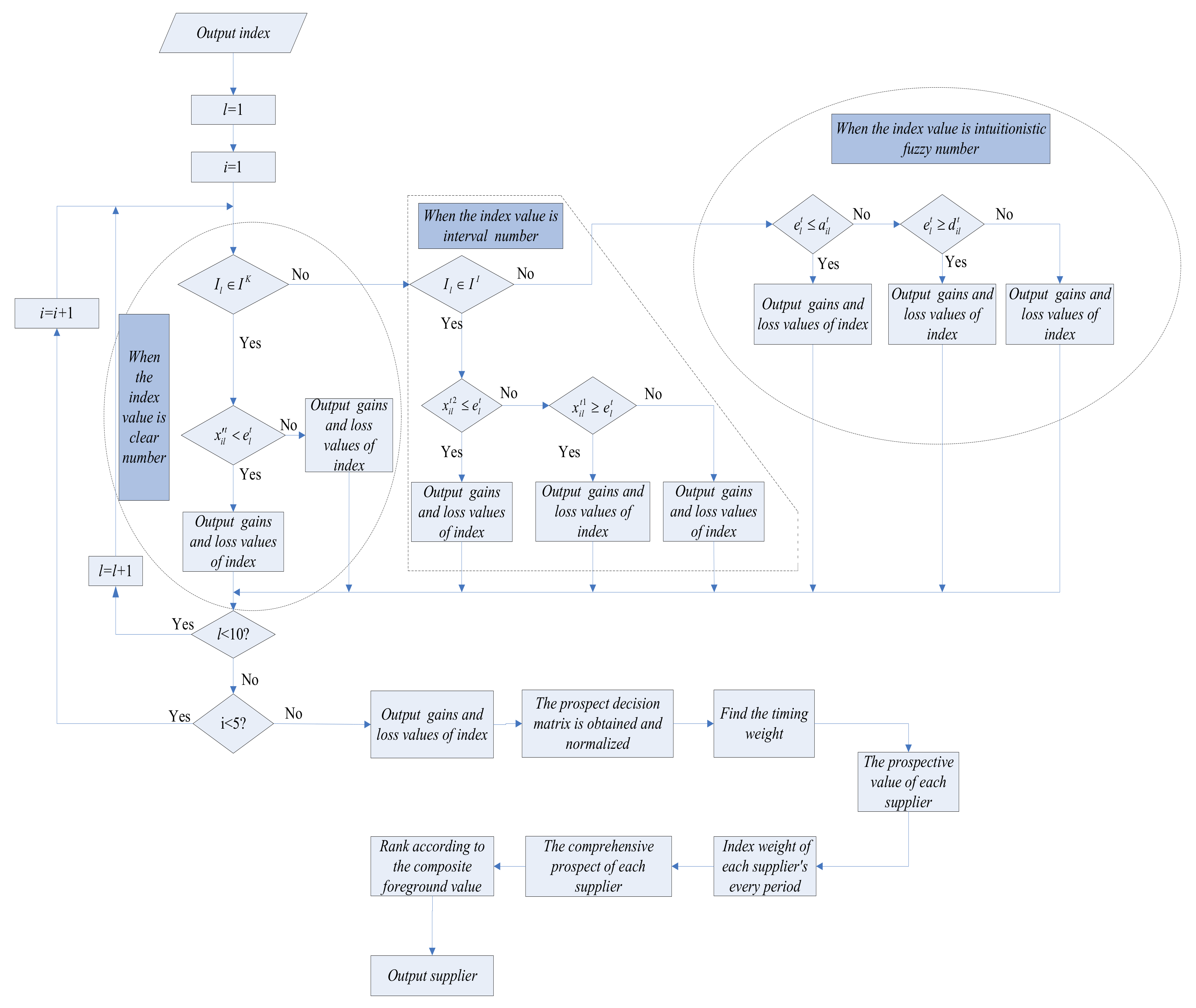
Table 1.
Evaluation criteria for green supplier selection.
| Index Type | Index Name |
|---|---|
| Cost index | Product prices: the prices of raw materials include both the price of the purchase itself and the cost of handling all kinds of emergencies in the production process. |
| Defective rate: the defective rate of raw materials directly affects the total purchase of the manufacturer. The provision of qualified raw materials is a basic requirement for manufacturer. | |
| Delivery cycle: the supply time of suppliers directly affects the production schedule and the manufacturer’s plan. | |
| Inventory costs: the suppliers’ level of inventory costs directly affects the direct costs of manufacturers. | |
| Poor environmental records: mainly refers to a history of environmental problems, with a bad record of legal penalties. | |
| Profitability index | After-sales service level: includes the performance of service commitments, the attitude and efficiency of after-sales service, customer satisfaction, etc. |
| Product environmental protection design ability: mainly refers to the product recycling and environmental protection ability. | |
| Research and innovation ability: it is not only critical to the survival of enterprises, but is also a key factor for manufacturing enterprises when choosing suppliers. | |
| Environmental efficiency: refers to the “three wastes” (waste gas, waste water and waste residues) emissions, and energy usage of the suppliers | |
| Resource recycling capacity: mainly refers to the ability of supplier to handle the defective product, the recycling goods, etc. |
Table 2.
The description of variables used.
| Variable | Meaning |
|---|---|
| A collection of alternative green suppliers | |
| A collection of indexes | |
| and | Profitability indexes, cost indexes |
| The weight vector of the indexes | |
| Natural state set | |
| and | The occurrence probability of state t |
| The vector of indicator expectation | |
| The decision makers’ expectations for index Il | |
| In the state t, the decision maker’s expectations for the index Il | |
| Risk decision matrix | |
| In the state t, the green supplier Si has the risk decision result for the index Il | |
| An indicator set whose value is clear numbers | |
| An indicator set whose value is interval numbers | |
| An indicator set whose value is intuitionistic fuzzy number | |
| Subscripted collections of index subset IK | |
| Subscripted collections of index subset IL | |
| Subscripted collections of index subset IF |
Table 3.
Green supplier evaluation-related data.
| Index | Statue | Probability | Green Suppliers | Exception | |||
|---|---|---|---|---|---|---|---|
| S1 | S2 | S3 | S4 | ||||
| I1 | A1 | 0.3 | 10 | 12 | 11 | 13 | 10 |
| A2 | 0.3 | 12 | 13 | 10 | 10 | 11 | |
| A3 | 0.2 | 13 | 11 | 13 | 12 | 12 | |
| A4 | 0.2 | 11 | 14 | 12 | 11 | 12 | |
| I2 | A1 | 0.3 | 0.05 | 0.02 | 0.05 | 0.08 | 0.05 |
| A2 | 0.3 | 0.05 | 0.07 | 0.05 | 0.07 | 0.06 | |
| A3 | 0.2 | 0.07 | 0.1 | 0.15 | 0.09 | 0.1 | |
| A4 | 0.2 | 0.09 | 0.11 | 0.11 | 0.1 | 0.1 | |
| I3 | A1 | 0.3 | 9 | 10 | 8 | 11 | 9 |
| A2 | 0.3 | 10 | 11 | 12 | 10 | 10 | |
| A3 | 0.2 | 11 | 9 | 10 | 12 | 11 | |
| A4 | 0.2 | 10 | 11 | 12 | 9 | 11 | |
| I4 | A1 | 0.3 | 9 | 10 | 11 | 10 | 9 |
| A2 | 0.3 | 10 | 11 | 9 | 11 | 10 | |
| A3 | 0.2 | 8 | 12 | 10 | 12 | 10 | |
| A4 | 0.2 | 11 | 10 | 12 | 9 | 10 | |
| I5 | A1 | 0.3 | (0.05, 0.06) | (0.04, 0.05) | (0.05, 0.06) | (0.03, 0.04) | 0.04 |
| A2 | 0.3 | (0.02, 0.03) | (0.02, 0.03) | (0.03, 0.04) | (0.03, 0.05) | 0.03 | |
| A3 | 0.2 | (0.04, 0.05) | (0.02, 0.03) | (0.05, 0.06) | (0.04, 0.05) | 0.05 | |
| A4 | 0.2 | (0.03, 0.04) | (0.03, 0.04) | (0.02, 0.04) | (0.01, 0.03) | 0.02 | |
| I6 | A1 | 0.3 | ([5, 6, 7, 8]; 0.7, 0.3) | ([5, 7, 8, 9]; 00.8, 0.2) | ([3, 4, 5, 6]; 0.6, 0.4) | ([4, 5, 6, 7]; 0.8, 0.2) | 5 |
| A2 | 0.3 | ([4, 6, 7, 8]; 0.6, 0.3) | ([5, 6, 8, 9]; 0.8, 0.2) | ([3, 4, 7, 8]; 0.6, 0.4) | ([5, 6, 7, 8]; 0.8,0.2) | 5 | |
| A3 | 0.2 | ([4, 5, 6, 7]; 0.8, 0.2) | ([3, 4, 5, 6]; 0.8, 0.2) | ([2, 4, 5, 6]; 0.6, 0.3) | ([1, 3, 4, 5]; 0.6, 0.3) | 5 | |
| A4 | 0.2 | ([2, 3, 5, 6]; 0.6, 0.3) | ([2, 4, 5, 6]; 0.6, 0.3) | ([4, 5, 6, 7]; 0.7, 0.2) | ([6, 7, 8, 9]; 0.8, 0.1) | 6 | |
| I7 | A1 | 0.3 | ([4, 5, 7, 8]; 0.8, 0.2) | ([4, 5, 6, 7]; 0.8, 0.2) | ([3, 4, 7, 8]; 0.6, 0.4) | ([4, 6, 7, 8]; 0.6, 0.3) | 4 |
| A2 | 0.3 | ([4, 5, 6, 7]; 0.8, 0.2) | ([3, 5, 6, 7]; 0.8, 0.2) | ([2, 4, 6, 7]; 0.8, 0.2) | ([3, 4, 6, 7]; 0.6, 0.2) | 5 | |
| A3 | 0.2 | ([2, 3, 4, 5]; 0.6, 0.3) | ([5, 6, 8, 9]; 0.8, 0.2) | ([6, 7, 8, 9]; 0.8, 0.1) | ([5, 6, 7, 8]; 0.7, 0.2) | 6 | |
| A4 | 0.2 | ([5, 6, 7, 8]; 0.8, 0.1) | ([3, 4, 5, 6]; 0.6, 0.2) | ([6, 7, 8, 9]; 0.8, 0.1) | ([6, 7, 8, 9]; 0.8, 0.2) | 6 | |
| I8 | A1 | 0.3 | ([5, 6, 7, 8]; 0.7, 0.3) | ([4, 5, 6, 7]; 0.7, 0.2) | ([4, 5, 6, 7]; 0.8, 2) | ([2, 4, 5, 6]; 0.6, 0.3) | 6 |
| A2 | 0.3 | ([3, 4, 5, 6]; 0.6, 0.2) | ([3, 4, 5, 6]; 0.8, 0.1) | ([4, 5, 6, 7]; 0.7, 0.2) | ([3, 4, 5, 6]; 0.6, 0.2) | 5 | |
| A3 | 0.2 | ([5, 6, 8, 9]; 0.8, 0.2) | ([3, 5, 6, 7]; 0.8, 0.2) | ([4, 5, 6, 7]; 0.7, 0.2) | ([3, 5, 6, 7]; 0.7, 0.2) | 5 | |
| A4 | 0.2 | ([5, 6, 7, 8]; 0.8, 0.1) | ([4, 5, 6, 7]; 0.8, 0.2) | ([2, 3, 4, 5]; 0.6, 0.4) | ([3, 5, 6, 7]; 0.8, 0.2) | 5 | |
| I9 | A1 | 0.3 | ([4, 5, 6, 7]; 0.7, 0.2) | ([3, 4, 7, 8]; 0.6, 0.3) | ([6, 7, 8, 9]; 0.8, 0.1) | ([3, 4, 5, 6]; 0.5, 0.4) | 6 |
| A2 | 0.3 | ([3, 4, 5, 6]; 0.6, 0.3) | ([2, 3, 4, 5]; 0.6, 0.3) | ([4, 5, 6, 7]; 0.8, 0.2) | ([3, 4, 6, 7]; 0.8,0.2) | 4 | |
| A3 | 0.2 | ([5, 6, 7, 8]; 0.7, 0.3) | ([6, 7, 8, 9]; 0.8, 0.1) | ([3, 4, 7, 8]; 0.6, 0.4) | ([3, 4, 5, 6]; 0.6, 0.4) | 5 | |
| A4 | 0.2 | ([3, 5, 6, 7]; 0.8, 0.2) | ([3, 4, 5, 6]; 0.6, 0.4) | ([3, 5, 6, 7]; 0.8, 0.2) | ([6, 7, 8, 9]; 0.8, 0.1) | 6 | |
| I10 | A1 | 0.3 | ([4, 5, 6, 7]; 0.8, 0.2) | ([3, 4, 7, 8]; 0.6, 0.3) | ([2, 3, 4, 5]; 0.6, 0.3) | ([4, 5, 6, 7]; 0.8, 0.2) | 6 |
| A2 | 0.3 | ([3, 4, 7, 8]; 0.6, 0.3) | ([6, 7, 8, 9]; 0.8, 0.1) | ([5, 6, 7, 8]; 0.8, 0.2) | ([3, 4, 6, 7]; 0.7, 0.2) | 5 | |
| A3 | 0.2 | ([6, 7, 8, 9]; 0.8, 0.1) | ([3, 4, 5, 6]; 0.6, 0.2) | ([5, 6, 7, 8]; 0.7, 0.2) | ([4, 5, 6, 7]; 0.7, 0.2) | 7 | |
| A4 | 0.2 | ([2, 3, 4, 5]; 0.7, 0.3) | ([6, 7, 8, 9]; 0.8, 0.1) | ([2, 3, 4, 5]; 0.6, 0.3) | ([5, 6, 7, 8]; 0.8, 0.2) | 5 | |
Table 4.
The prospect index value of the green supplier.
| Index | Statue | Probability | Suppliers (Prospect Value of Index) | |||
|---|---|---|---|---|---|---|
| S1 | S2 | S3 | S4 | |||
| I1 | A1 | 0.02342 | 0.00000 | −1.35644 | −0.73705 | −1.93803 |
| A2 | 0.02778 | −0.73705 | −1.35644 | 0.31837 | 0.31837 | |
| A3 | 0.02503 | −0.57831 | 0.26076 | −0.57831 | 0.00000 | |
| A4 | 0.02793 | 0.26076 | −1.06430 | 0.00000 | 0.26076 | |
| I2 | A1 | 0.02608 | 0.00000 | 0.01455 | 0.00000 | −0.03368 |
| A2 | 0.02896 | 0.00553 | −0.01281 | 0.00553 | −0.01281 | |
| A3 | 0.02426 | 0.01192 | 0.00000 | −0.04142 | 0.00453 | |
| A4 | 0.02519 | 0.00453 | −0.01005 | −0.01005 | 0.00000 | |
| I3 | A1 | 0.02384 | 0.00000 | −0.73705 | 0.31837 | −1.35644 |
| A2 | 0.02775 | 0.00000 | −0.73705 | −1.35644 | 0.00000 | |
| A3 | 0.02417 | 0.00000 | 0.47990 | 0.26076 | −0.57831 | |
| A4 | 0.02395 | 0.26076 | 0.00000 | −0.57831 | 0.47990 | |
| I4 | A1 | 0.02538 | 0.00000 | −0.73705 | −1.35644 | −0.73705 |
| A2 | 0.02485 | 0.00000 | −0.73705 | 0.31837 | −0.73705 | |
| A3 | 0.02449 | 0.47990 | −1.06430 | 0.00000 | −1.06430 | |
| A4 | 0.02409 | −0.57831 | 0.00000 | −1.06430 | 0.26076 | |
| I5 | A1 | 0.02557 | −0.01830 | −0.00696 | −0.01830 | 0.00301 |
| A2 | 0.02811 | 0.00301 | 0.00301 | −0.00696 | −0.01281 | |
| A3 | 0.02607 | 0.00246 | 0.01015 | −0.00546 | 0.00246 | |
| A4 | 0.02595 | −0.01436 | −0.01436 | −0.01850 | −0.00163 | |
| I6 | A1 | 0.02358 | 0.72558 | 1.31227 | −0.79169 | 0.25325 |
| A2 | 0.02377 | 1.01138 | 1.35835 | 0.20373 | 0.76301 | |
| A3 | 0.02390 | 0.21267 | −0.64137 | −1.07268 | 0.00000 | |
| A4 | 0.02536 | 0.00000 | 0.00000 | −0.62847 | 0.62495 | |
| I7 | A1 | 0.02387 | 1.26596 | 0.76301 | 1.89386 | 1.19607 |
| A2 | 0.02377 | 0.25325 | −0.11030 | −1.04971 | −0.47233 | |
| A3 | 0.02407 | 0.00000 | 0.83133 | 0.62495 | 0.32107 | |
| A4 | 0.02805 | 0.20154 | −0.11953 | 0.62495 | 0.62495 | |
| I8 | A1 | 0.02380 | 0.23966 | −0.80721 | −0.82297 | 0.00000 |
| A2 | 0.02478 | −0.79169 | −0.82297 | 0.23966 | −0.79169 | |
| A3 | 0.02353 | 1.11257 | −0.07258 | 0.20154 | −0.08371 | |
| A4 | 0.02399 | 0.62495 | 0.21267 | 0.00000 | −0.07258 | |
| I9 | A1 | 0.02338 | −0.80721 | −1.84648 | 0.76301 | 0.00000 |
| A2 | 0.02405 | 0.22601 | −0.79169 | 0.76301 | 1.00858 | |
| A3 | 0.02386 | 0.59429 | 0.97966 | 0.19956 | −0.61575 | |
| A4 | 0.02393 | −1.09904 | 0.00000 | −1.09904 | 0.62495 | |
| I10 | A1 | 0.02513 | −0.82297 | −1.84648 | 0.00000 | −0.82297 |
| A2 | 0.02364 | 0.20373 | 1.19607 | 0.76301 | −0.47233 | |
| A3 | 0.02585 | 0.21267 | 0.00000 | −0.62847 | 0.00000 | |
| A4 | 0.02480 | 0.00000 | 0.97966 | 0.00000 | 0.62495 | |
Table 5.
The penalty function of green suppliers.
| Index | Statue | Probability | Suppliers (Penalty Function) | |||
|---|---|---|---|---|---|---|
| S1 | S2 | S3 | S4 | |||
| I1 | A1 | 0.02342 | 1.00000 | 0.98394 | 1.00000 | 0.95419 |
| A2 | 0.02778 | 0.98318 | 0.94497 | 1.00000 | 1.00000 | |
| A3 | 0.02503 | 0.98181 | 1.00000 | 0.98348 | 1.00000 | |
| A4 | 0.02793 | 1.00000 | 0.94529 | 0.98192 | 1.00000 | |
| I2 | A1 | 0.02608 | 1.00000 | 1.00000 | 1.00000 | 0.94754 |
| A2 | 0.02896 | 1.00000 | 0.97684 | 1.00000 | 0.97855 | |
| A3 | 0.02426 | 1.00000 | 0.98130 | 0.95116 | 1.00000 | |
| A4 | 0.02519 | 1.00000 | 0.98147 | 0.97693 | 1.00000 | |
| I3 | A1 | 0.02384 | 1.00000 | 0.98491 | 1.00000 | 0.95226 |
| A2 | 0.02775 | 1.00000 | 0.98052 | 0.94285 | 1.00000 | |
| A3 | 0.02417 | 0.98316 | 1.00000 | 1.00000 | 0.95652 | |
| A4 | 0.02395 | 1.00000 | 0.98036 | 0.95086 | 1.00000 | |
| I4 | A1 | 0.02538 | 1.00000 | 1.00000 | 0.95037 | 1.00000 |
| A2 | 0.02485 | 1.00000 | 0.98474 | 1.00000 | 0.98388 | |
| A3 | 0.02449 | 1.00000 | 0.98362 | 1.00000 | 0.98475 | |
| A4 | 0.02409 | 0.98352 | 1.00000 | 0.95619 | 1.00000 | |
| I5 | A1 | 0.02557 | 0.98290 | 1.00000 | 0.98409 | 1.00000 |
| A2 | 0.02811 | 1.00000 | 1.00000 | 0.98033 | 0.94548 | |
| A3 | 0.02607 | 1.00000 | 1.00000 | 0.94650 | 1.00000 | |
| A4 | 0.02595 | 1.00000 | 1.00000 | 0.95045 | 1.00000 | |
| I6 | A1 | 0.02358 | 1.00000 | 1.00000 | 0.95370 | 0.98645 |
| A2 | 0.02377 | 1.00000 | 1.00000 | 0.95232 | 0.98089 | |
| A3 | 0.02390 | 1.00000 | 0.98618 | 0.95564 | 1.00000 | |
| A4 | 0.02536 | 1.00000 | 1.00000 | 0.94987 | 1.00000 | |
| I7 | A1 | 0.02387 | 1.00000 | 0.95376 | 1.00000 | 0.98426 |
| A2 | 0.02377 | 1.00000 | 1.00000 | 0.95645 | 0.97876 | |
| A3 | 0.02407 | 0.95366 | 1.00000 | 1.00000 | 0.98271 | |
| A4 | 0.02805 | 0.98307 | 0.94543 | 1.00000 | 1.00000 | |
| I8 | A1 | 0.02380 | 1.00000 | 0.98433 | 0.95211 | 1.00000 |
| A2 | 0.02478 | 1.00000 | 0.95162 | 1.00000 | 1.00000 | |
| A3 | 0.02353 | 1.00000 | 0.98595 | 1.00000 | 0.95533 | |
| A4 | 0.02399 | 1.00000 | 1.00000 | 0.98237 | 0.95494 | |
| I9 | A1 | 0.02338 | 0.98611 | 0.95830 | 1.00000 | 1.00000 |
| A2 | 0.02405 | 0.98565 | 0.95609 | 1.00000 | 1.00000 | |
| A3 | 0.02386 | 1.00000 | 1.00000 | 0.98673 | 0.95205 | |
| A4 | 0.02393 | 0.98076 | 1.00000 | 0.98335 | 1.00000 | |
| I10 | A1 | 0.02513 | 1.00000 | 0.95240 | 1.00000 | 1.00000 |
| A2 | 0.02364 | 0.98226 | 1.00000 | 1.00000 | 0.95614 | |
| A3 | 0.02585 | 1.00000 | 1.00000 | 0.94947 | 1.00000 | |
| A4 | 0.02480 | 0.98167 | 1.00000 | 0.98095 | 1.00000 | |
Table 6.
The timing weight of green suppliers at each period.
| S1 | S2 | S3 | S4 | |
|---|---|---|---|---|
| A1 | 0.69793 | 0.69663 | 0.69832 | 0.69667 |
| A2 | 0.14829 | 0.14755 | 0.14770 | 0.14860 |
| A3 | 0.08680 | 0.08814 | 0.08669 | 0.08714 |
| A4 | 0.06045 | 0.06079 | 0.05994 | 0.06138 |
Table 7.
The comprehensive prospect of green suppliers.
| Value of the Time Attenuation Factor | Comprehensive Prospect Value of Suppliers | Results | |||
|---|---|---|---|---|---|
| 0.01489 | −0.09507 | −0.0186 | −0.06297 | ||
| 0.01299 | −0.09601 | −0.01982 | −0.05846 | ||
| 0.01306 | −0.08817 | −0.02007 | −0.05228 | ||
| 0.01314 | −0.08251 | −0.02036 | −0.04781 | ||
Table 8.
Comparison result of the proposed method with the Technique for Order Preference by Similarity to an Ideal Solution (TOPSIS) and the variable weight dynamic multi-attribute method.
Table 8.
Comparison result of the proposed method with the Technique for Order Preference by Similarity to an Ideal Solution (TOPSIS) and the variable weight dynamic multi-attribute method.
| Method | Evaluation Results |
|---|---|
| TOPSIS | |
| Dynamic multi-attribute decision-making method | |
| Generalized Ordinal Number Based on the Third Generation Prospect Theory |
© 2018 by the authors. Licensee MDPI, Basel, Switzerland. This article is an open access article distributed under the terms and conditions of the Creative Commons Attribution (CC BY) license (http://creativecommons.org/licenses/by/4.0/).
Share and Cite
MDPI and ACS Style
Song, W.; Chen, Z.; Liu, A.; Zhu, Q.; Zhao, W.; Tsai, S.-B.; Lu, H. A Study on Green Supplier Selection in Dynamic Environment. Sustainability 2018, 10, 1226. https://doi.org/10.3390/su10041226
AMA Style
Song W, Chen Z, Liu A, Zhu Q, Zhao W, Tsai S-B, Lu H. A Study on Green Supplier Selection in Dynamic Environment. Sustainability. 2018; 10(4):1226. https://doi.org/10.3390/su10041226
Chicago/Turabian StyleSong, Wei, Zhiya Chen, Aijun Liu, Qiuyun Zhu, Wei Zhao, Sang-Bing Tsai, and Hui Lu. 2018. "A Study on Green Supplier Selection in Dynamic Environment" Sustainability 10, no. 4: 1226. https://doi.org/10.3390/su10041226
Note that from the first issue of 2016, this journal uses article numbers instead of page numbers. See further details here.