Typically Diverse: The Nature of Urban Agriculture in South Australia

Abstract
:1. Introduction
2. Materials and Methods
3. Results
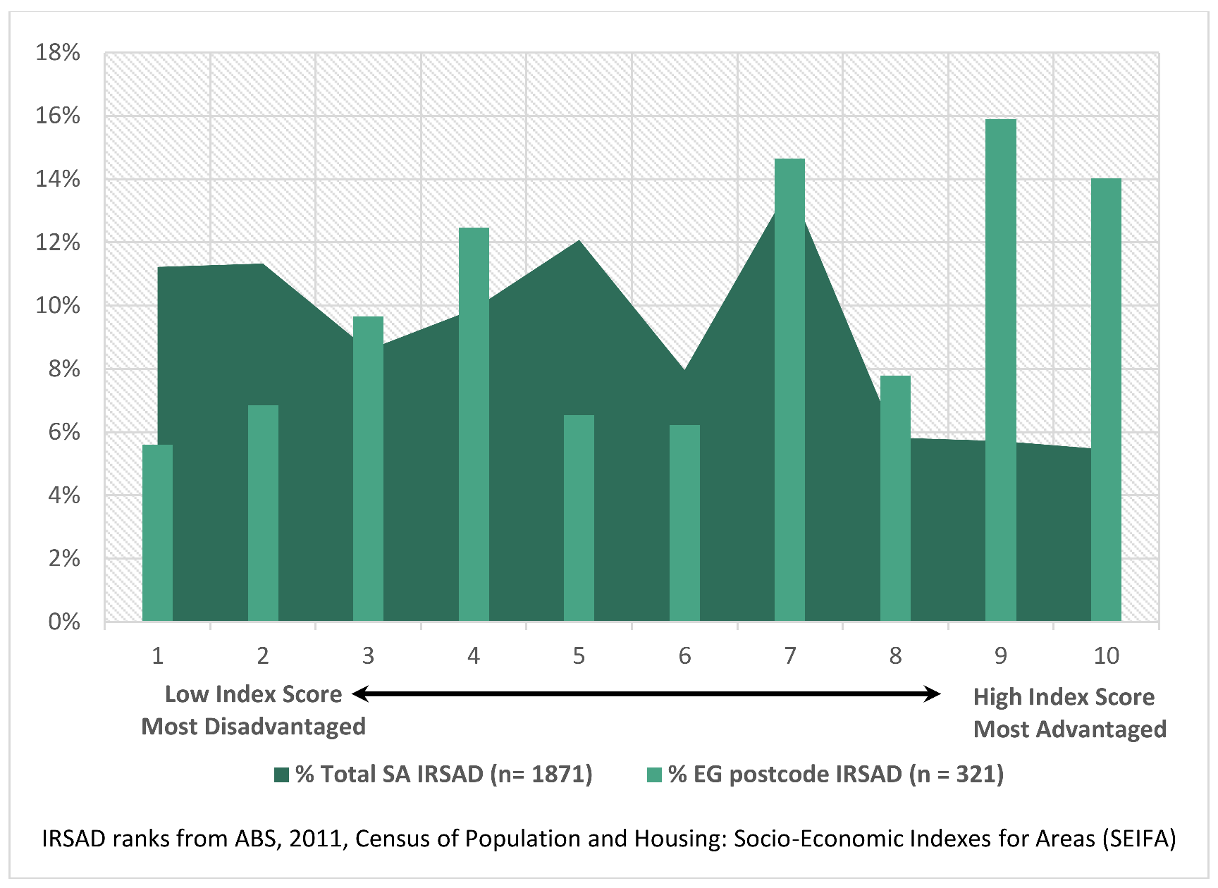
3.1. Demographics
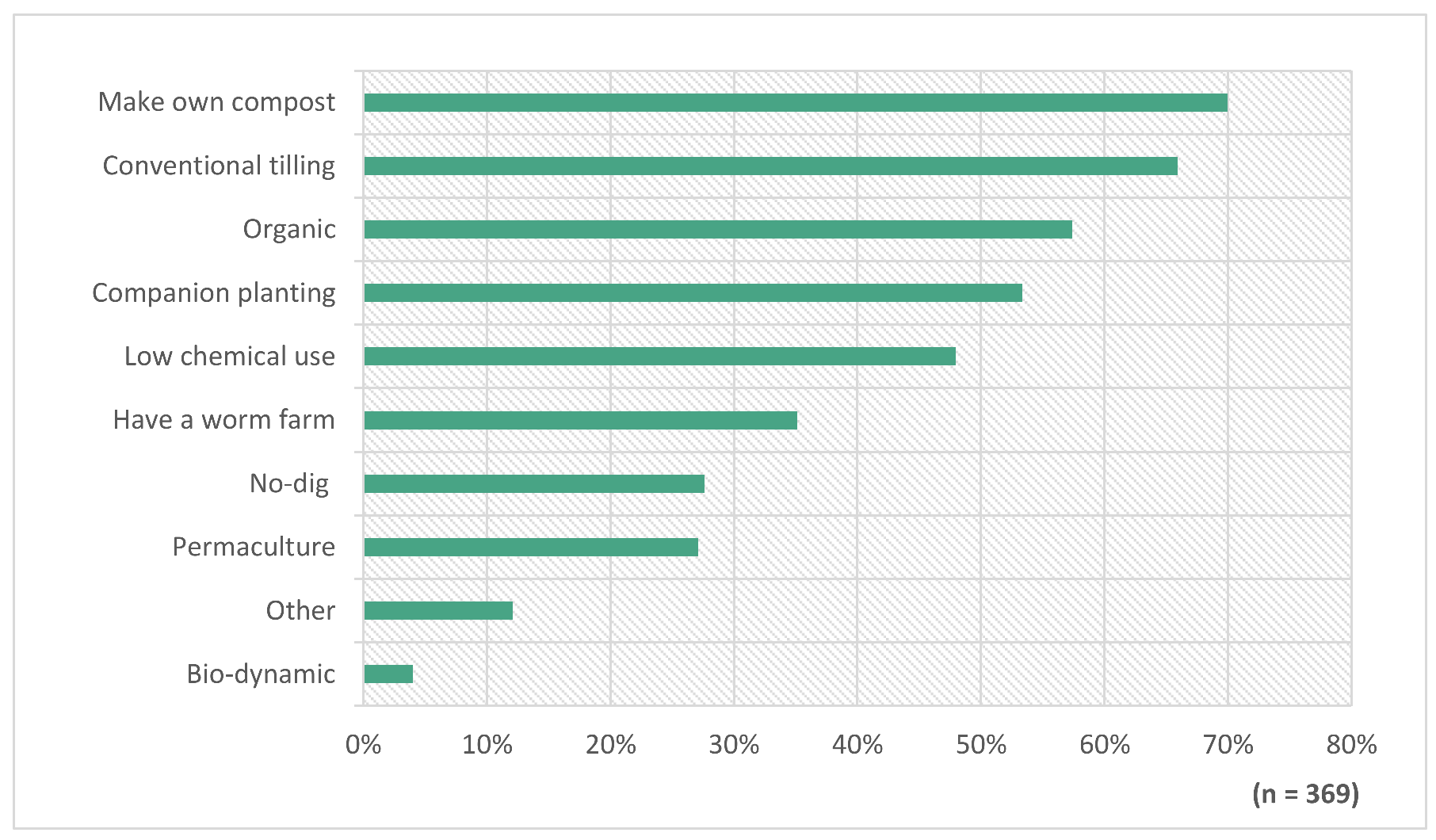
3.2. Gardening Background and Approaches
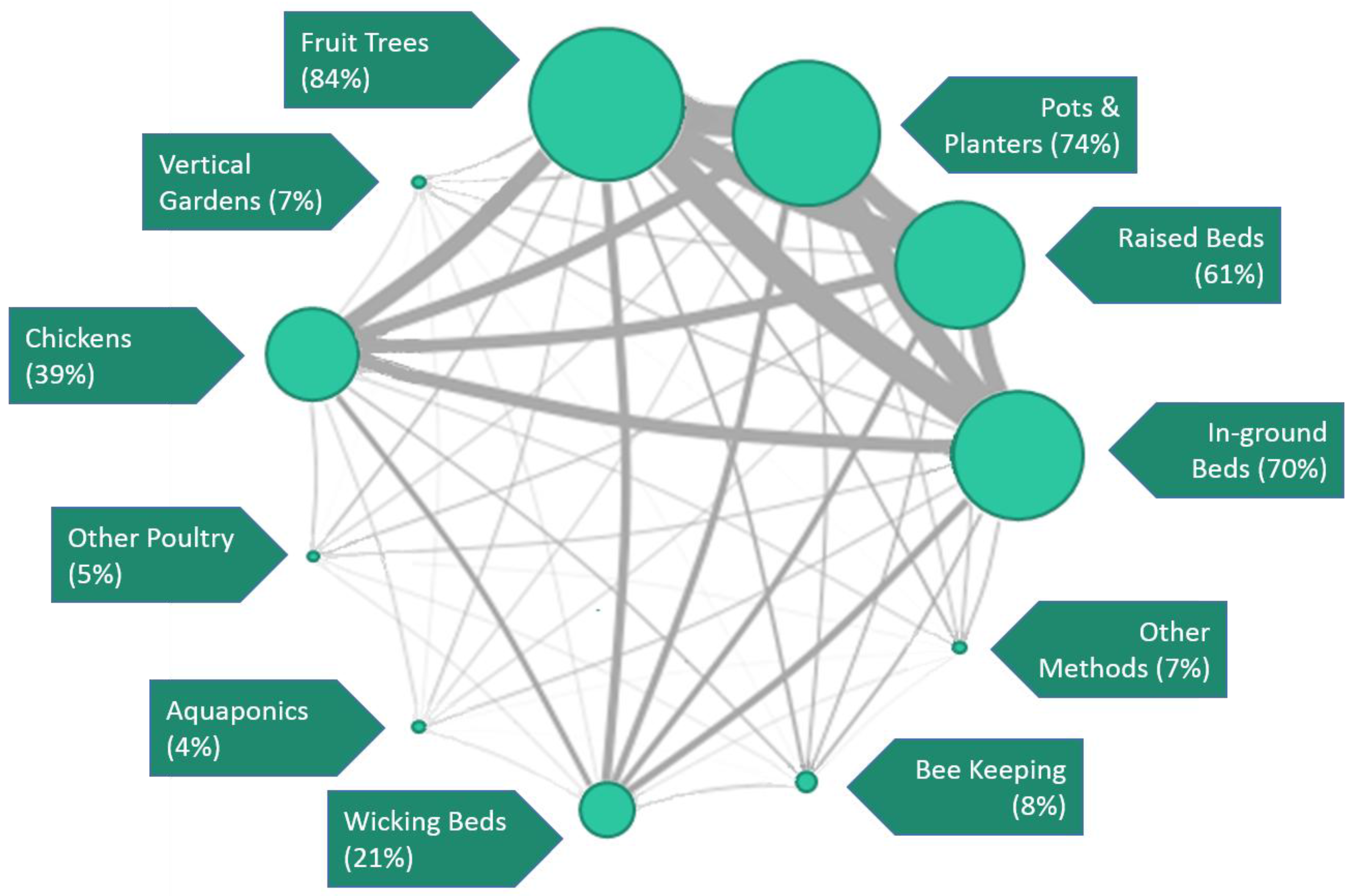
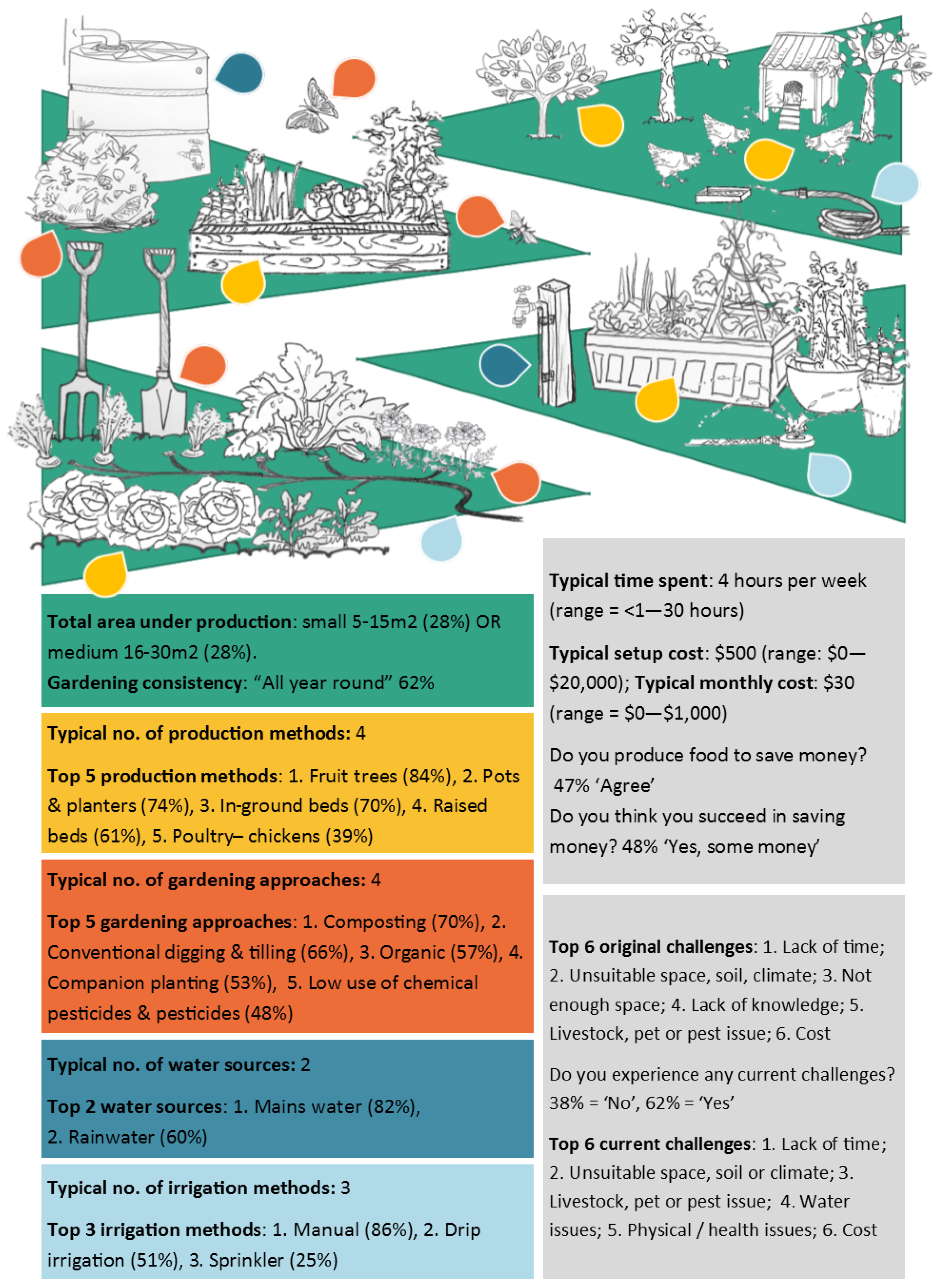
3.3. Physical Elements of the Food Gardens
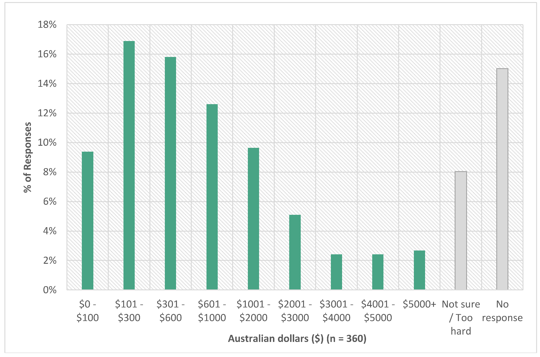
3.4. Garden Inputs
3.5. Theoretical Comparison Results
4. Discussion
4.1. South Australian Home Food Gardens
4.2. Differences between the ‘Optimized Garden Model’ and the EG Survey Data
4.3. Challenges to Home Food Gardening
4.4. Implications for Economic Sustainability of Home Food Gardens
4.5. Recommendations for Future Work
5. Conclusions
Supplementary Materials
Acknowledgments
Author Contributions
Conflicts of Interest
References
- Pearson, L.J.; Pearson, L.; Pearson, C.J. Sustainable urban agriculture: Stocktake and opportunities. Int. J. Agric. Sustain. 2010, 8, 7–19. [Google Scholar] [CrossRef]
- Farrell, B. A place for food within sustainable urban masterplanning. In Building Sustainable Cities of the Future; Bishop, J., Ed.; Springer: Cham, Switzerland, 2017; pp. 117–140. [Google Scholar]
- Pires, V. Planning for urban agriculture planning in Australian cities. In Proceedings of the State of Australian Cities Conference (SOAC), Sydney, NSW, Australia, 26–29 November 2013. [Google Scholar]
- Burton, P.; Lyons, K.; Richards, C.; Amati, M.; Rose, N.; Desfours, L.; Pires, V.; Barclay, R. Urban Food Security, Urban Resilience and Climate Change; National Climate Change Adaption Research Facility: Gold Coast, Australia, 2013; p. 160. [Google Scholar]
- Deelstra, T.; Girardet, H. Urban agriculture and sustainable cities. In Growing Cities, Growing Food: Urban Agriculture on the Policy Agenda; Bakker, N., Dubbeling, M., Gündel, S., Sabel-Koshella, U., de Zeeuw, H., Eds.; Sentralstelle für Ernährung und Landwirtschaft (ZEL): Feldafing, Germany, 2000; pp. 43–66. [Google Scholar]
- Smit, J.; Nasr, J. Urban agriculture for sustainable cities: Using wastes and idle land and water bodies as resources. Environ. Urban. 1992, 4, 141–152. [Google Scholar] [CrossRef]
- Butterfield, B. The Impact of Home and Community Gardening in America; National Gardening Association: South Burlington, VT, USA, 2009. [Google Scholar]
- Taylor, J.; Lovell, S. Urban home food gardens in the global north: Research traditions and future directions. Agric. Hum. Values 2013, 31, 285–305. [Google Scholar] [CrossRef]
- Wise, P. Grow Your Own: The Potential Value and Impacts of Residential and Community Food Gardening; 59; The Australia Institute: Canberra, Australia, 2014. [Google Scholar]
- Conway, T.; Brannen, K. Who is tending their garden? Edible gardens as a residential landscaping choice. Cities Environ. 2014, 7, 10. [Google Scholar]
- Mok, H.-F.; Williamson, V.G.; Grove, J.R.; Burry, K.; Barker, S.F.; Hamilton, A.J. Strawberry fields forever? Urban agriculture in developed countries: A review. Agron. Sustain. Dev. 2014, 34, 21–43. [Google Scholar] [CrossRef]
- Pollard, G.; Roetman, P.; Ward, J. The case for citizen science in urban agriculture research. Future Food J. Food Agric. Soc. 2017, 5, 9–20. [Google Scholar]
- Gray, L.; Guzman, P.; Glowa, K.; Drevno, A. Can home gardens scale up into movements for social change? The role of home gardens in providing food security and community change in San Jose, California. Local Environ. 2014, 19, 187–203. [Google Scholar] [CrossRef]
- Ward, J.; Ward, P.; Mantzioris, E.; Saint, C. Optimising diet decisions and urban agriculture using linear programming. Food Secur. 2014, 6, 701–718. [Google Scholar] [CrossRef]
- Kortright, R.; Wakefield, S. Edible backyards: A qualitative study of household food growing and its contributions to food security. Agric. Hum. Values 2011, 28, 39–53. [Google Scholar] [CrossRef]
- Cleveland, D.; Orum, T.; Ferguson, N. Economic value of home vegetable gardens in an urban desert environment. Hortic. Sci. 1985, 20, 694–696. [Google Scholar]
- Stall, W.M. Economic value of a home vegetable garden in South Florida. Proc. Fla. State Hortic. Soc. 1979, 92, 213–214. [Google Scholar]
- Stephens, J.M.; Carter, L.; Van Gundy, C. Economic value of vegetables grown in North Florida gardens. Proc. Fla. State Hortic. Soc. 1980, 93, 70–72. [Google Scholar]
- Utzinger, J.; Connolly, H. Economic value of a home vegetable garden. HortScience 1978, 13, 148–149. [Google Scholar]
- Algert, S.J.; Baameur, A.; Renvall, M.J. Vegetable output and cost savings of community gardens in San Jose, California. J. Acad. Nutr. Diet. 2014, 114, 1072–1076. [Google Scholar] [CrossRef] [PubMed]
- Gittleman, M.; Jordan, K.; Brelsford, E. Using citizen science to quantify community garden crop yields. Cities Environ. 2012, 5, 4. [Google Scholar] [CrossRef]
- Pourias, J.; Duchemin, E.; Aubry, C. Products from urban collective gardens: Food for thought or for consumption? Insights from Paris and Montreal. J. Agric. Food Syst. Community Dev. 2015, 5, 1–25. [Google Scholar] [CrossRef]
- Vitiello, D.; Nairn, M.; Grisso, J.; Swistak, N. Community Gardening in Camden, NJ Harvest Report: Summer 2009; Penn’s Center for Public Health Initiatives: Philadelphia, PA, USA, 2010. [Google Scholar]
- Vitiello, D.; Nairn, M.; Planning, P. Community Gardening in Philadelphia: 2008 Harvest Report. 2009. Available online: http://www.farmlandinfo.org/sites/default/files/Philadelphia_Harvest_1.pdf (accessed on 5 June 2016).
- Codyre, M.; Fraser, E.; Landman, K. How does your garden grow? An empirical evaluation of the costs and potential of urban gardening. Urban For. Urban Green. 2014, 14, 72–79. [Google Scholar] [CrossRef]
- Conk, S. Quantifying Yields of Home and Community Gardens in Laramie, Wyoming; University of Wyoming: Laramie, WY, USA, 2015. [Google Scholar]
- Zainuddin, Z.; Mercer, D. Domestic residential garden food production in Melbourne, Australia: A fine-grained analysis and pilot study. Aust. Geogr. 2014, 45, 465–484. [Google Scholar] [CrossRef]
- Doiron, R. What’s a Home Garden Worth? Available online: http://kgi.org/blogs/roger-doiron/home-garden-worth (accessed on 7 March 2009).
- French, J. Backyard Self-Sufficiency, 2nd ed.; Aird Books: Melbourne, Australia, 2009. [Google Scholar]
- West, P. How growing your own will save you a packet. ABC Organic Gardening Magazine, 2018; 42–45. [Google Scholar]
- Dewaelheyns, V.; Lerouge, F.; Rogge, E.; Vranken, L. Garden Space: Mapping Trade-Offs and the Adaptive Capacity of Home Food Production; Department of Earth and Environmental Sciences, University of Leuvan: Leuvan, Belgium, 2014; p. 34. [Google Scholar]
- Colasanti, K.; Hamm, M. Assessing the local food supply capacity of Detroit, Michigan. J. Agric. Food Syst. Community Dev. 2010, 1. [Google Scholar] [CrossRef]
- Ackerman, K. The Potential for Urban Agriculture in New York City: Growing Capacity, Food Security, & Green Infrastructure; Urban Design Lab at the Earth Institute Columbia University: New York, NY, USA, 2011. [Google Scholar]
- Ward, J.; Symons, J. Optimising crop selection for small urban food gardens in dry climates. Horticulturae 2017, 3, 33. [Google Scholar] [CrossRef]
- The Economist Intelligence Unit. Global Food Security Index; Du Pont: New York, NY, USA, 2007. [Google Scholar]
- United States Department of Agriculture (USDA). Food Expenditures; Economic Research Service, Ed.; USDA: Washington, DC, USA, 2017.
- Australian Bureau of Statistics (ABS). Water Account Australia 2013–2014, Cat No 4610.0; Australian Bureau of Statistics (ABS), Ed.; Commonwealth of Australia: Canberra, Australia, 2015.
- SA Water. Residential Water Prices. Available online: https://www.sawater.com.au/accounts-and-billing/current-water-and-sewerage-rates/residential-water-supply (accessed on 19 July 2016).
- Bureau of Meteorology. Adelaide (Kent town) 1977–2016: Climate Statistics for Australian Locations. Available online: http://www.bom.gov.au/climate/averages/tables/cw_023090_All.shtml (accessed on 12 November 2016).
- Ward, J.; Ward, P.; Saint, C.; Mantzioris, E. The urban agriculture revolution: Implications for water use in cities. Water J. Aust. Water Assoc. 2014, 41, 69–74. [Google Scholar]
- R Core Team. R: A Language and Environment for Statistical Computing; R Foundation for Statistical Computing: Vienna, Austria, 2017. [Google Scholar]
- Butts, C. Network: Classes for Relational Data, R Package Version 1.13.0; The Statnet Project; Available online: http://statnet.org (accessed on 12 July 2016).
- Butts, C. Network: A package for managing relational data in R. J. Stat. Softw. 2008, 24. [Google Scholar] [CrossRef]
- Australian Bureau of Statistics (ABS). Education and Work, Australia, May 2016; Cat No. 6227.0; Australian Bureau of Statistics (ABS), Ed.; Commonwealth of Australia: Canberra, Australia, 2016.
- Rur, M. Measuring Garden Footprints. Master’s Thesis, Swedish University of Agricultural Sciences, Uppsala, Sweden, 2010. [Google Scholar]
- Auricht, G. Food glorious food. In Adelaide: Water of a City; Daniels, C., Ed.; Wakefield Press: Adelaide, Australia, 2010; pp. 315–344. [Google Scholar]
- Gaynor, A. Harvest of the Suburbs: An Environmental History of Growing Food in Australian Cities; University of Western Australia Press: Crawley, Australia, 2006. [Google Scholar]
- Australian Bureau of Statistics (ABS). Water Account Australia 2014–2015; Cat No 4610.0; Australian Bureau of Statistics (ABS), Ed.; Commonwealth of Australia: Canberra, Australia, 2016.
- Fortier, J.-M. The Market Gardener: A Successful Grower’s Handbook for Small-Scale Organic Farming; New Society Publishers: Gabriola Island, BC, Canada, 2014. [Google Scholar]
- Conway, T. Home-based edible gardening: Urban residents’ motivations and barriers. Cities Environ. 2016, 9, 3. [Google Scholar]
- Newman, L. Extreme local food: Two case studies in assisted urban small plot intensive agriculture. Environments 2008, 36, 33. [Google Scholar]
- Zahina-Ramos, J. Attitudes and Perspectives about Backyard Food Gardening: A Case Study in South Florida. Ph.D. Thesis, Florida Atlantic University, Boca Raton, FL, USA, 2013. [Google Scholar]
- Langellotto, G.A. What are the economic costs and benefits of home vegetable gardens? J. Ext. 2014, 52, 2. [Google Scholar]
- Yates, J. Abundance on trial: The cultural signifiance of sustainability. Hedgehog Rev. 2012, 14, 8–25. [Google Scholar]
- Block, K.; Gibbs, L.; Staiger, P.; Gold, L.; Johnson, B.; Macfarlane, S.; Long, C.; Townsend, M. Growing community: The impact of the stephanie alexander kitchen garden program on the social and learning environment in primary schools. Health Educ. Behav. 2012, 39, 419–432. [Google Scholar] [CrossRef] [PubMed]
- Alaimo, K.; Packnett, E.; Miles, R.A.; Kruger, D.J. Fruit and vegetable intake among urban community gardeners. J. Nutr. Educ. Behav. 2008, 40, 94–101. [Google Scholar] [CrossRef] [PubMed]
- Kingsley, J.; Townsend, M. ‘Dig in’ to social capital: Community gardens as mechanisms for growing urban social connectedness. Urban Policy Res. 2006, 24, 525–537. [Google Scholar] [CrossRef]
- Zick, C.; Smith, K.; Kowaleski-Jones, L.; Uno, C.; Merrill, B. Harvesting more than vegetables: The potential weight control benefits of community gardening. Am. J. Public Health 2013, 103, 1110–1115. [Google Scholar] [CrossRef] [PubMed]
- Soga, M.; Cox, D.T.C.; Yamaura, Y.; Gaston, K.J.; Kurisu, K.; Hanaki, K. Health benefits of urban allotment gardening: Improved physical and psychological well-being and social integration. Int. J. Environ. Res. Public Health 2017, 14, 71. [Google Scholar] [CrossRef] [PubMed]
- Wood, C.J.; Pretty, J.; Griffin, M. A case-control study of the health and well-being benefits of allotment gardening. J. Public Health 2016, 38, 336–344. [Google Scholar] [CrossRef] [PubMed]


| Responses | Home Owners (n = 278) | Home Renters (n = 36) | Lowest 2 IRSAD Scores (n = 39) | Highest 2 IRSAD Scores (n = 76) |
|---|---|---|---|---|
| Strongly Disagree | 2% | 3% | 3% | 3% |
| Disagree | 12% | 8% | 8% | 14% |
| Neutral | 30% | 19% | 15% | 32% |
| Agree | 42% | 33% | 49% | 41% |
| Strongly Agree | 14% | 36% | 26% | 11% |
| Initial Challenges (n = 904) | % | Current Challenges (n = 272) | % | ||
|---|---|---|---|---|---|
| 1 | Lack of time | 50 | 1 | Lack of time | 28 |
| 2 | Unsuitable conditions | 36 | 2 | Unsuitable conditions | 21 |
| 3 | Lack of knowledge | 28 | 3 | Water issues | 12 |
| 4 | Lack of space | 25 | 4 | Livestock, pet, or pest issues | 12 |
| 5 | Cost | 20 | 5 | Physical or health issues | 11 |
| 6 | Water issues | 17 | 6 | Lack of space | 8 |
| Is there currently anything that makes it difficult for you to continue to grow food? ‘Yes’ = 61%, ‘No’ = 38% (n = 376) | |||||
| Available Responses | Responses (n = 358) |
|---|---|
| Unsure | 14% |
| No, I know I don’t save money | 6% |
| No, I don’t think I save money | 14% |
| I think we break even | 12% |
| Yes, 0–5% of my weekly household produce budget | 13% |
| Yes, 6–25% of my weekly household produce budget | 15% |
| Yes, 26–75% of my weekly household produce budget | 16% |
| Yes, over 75% of my weekly household produce budget | 4% |
© 2018 by the authors. Licensee MDPI, Basel, Switzerland. This article is an open access article distributed under the terms and conditions of the Creative Commons Attribution (CC BY) license (http://creativecommons.org/licenses/by/4.0/).
Share and Cite
Pollard, G.; Ward, J.; Roetman, P. Typically Diverse: The Nature of Urban Agriculture in South Australia. Sustainability 2018, 10, 945. https://doi.org/10.3390/su10040945
Pollard G, Ward J, Roetman P. Typically Diverse: The Nature of Urban Agriculture in South Australia. Sustainability. 2018; 10(4):945. https://doi.org/10.3390/su10040945
Chicago/Turabian StylePollard, Georgia, James Ward, and Philip Roetman. 2018. "Typically Diverse: The Nature of Urban Agriculture in South Australia" Sustainability 10, no. 4: 945. https://doi.org/10.3390/su10040945