Integrated Harvest and Distribution Scheduling with Time Windows of Perishable Agri-Products in One-Belt and One-Road Context

1
Department of Management Engineering, Nanjing Agricultural University, Nanjing 210031, China
2
School of Business, Dalian University of Technology, Panjin 124221, China
*
Author to whom correspondence should be addressed.
Sustainability 2018, 10(5), 1570; https://doi.org/10.3390/su10051570
Submission received: 28 February 2018
/
Revised: 7 May 2018
/
Accepted: 7 May 2018
/
Published: 15 May 2018
(This article belongs to the Special Issue Sustainable Agribusiness Decision making model in Belt and Road Green Development)
Abstract
:The unique characteristics of perishable agri-products are a short lifespan and rapid quality deterioration. This establishes the need to significantly reduce the time from harvest to distribution. These features require reducing the processing time from harvest to distribution to being as short as possible. In this study, we focus on an integrated perishable agri-products scheduling problem that combines harvest and distribution simultaneously, with the purpose of reducing processing time and quality decay. We propose this problem as a mixed integer nonlinear programming model (MINLP) to optimize the harvest time and the vehicle routing to consumers, and this MINIP is formulated as a vehicle routing problem with time windows (VRPTW). We introduce a big M method to transform the nonlinear model into a linear model, then apply CPLEX to solve the transformed model. Numerical experiments and sensitive analysis are conducted to verify the efficiency of the proposed model and to provide managerial insights.
1. Introduction
In recent years, the Chinese government has adopted a number of policies to promote the opening up of the country and economic cooperation with other countries under the One-Belt and One-Road (OBOR) national strategy. This strategy can not only accelerate sustainable development but can also enhance international trade. China is one of the largest agricultural producing countries in the world. According to reports, the export of agri-products was at ¥11,209.1 billion in 2016, which was an increment of up from ¥503.49 billion as compared to the exports in 2015 [1]. Perishable agri-products are not only necessary for people’s daily lives but also an essential source of increasing income for peasant farmers. However, the short lifespan and quality decay nature of perishable agri-products make its deterioration rapid over time. According to an FAO report, the decay rate of perishable agri-products is about 1.7–5% in developed countries, while it is up to 20–30% along the farm-to-door supply chain in China [2]. Moreover, the ratio of social logistics costs in the gross domestic product is almost two-times higher than developed countries [3]. Therefore, reducing quality decay and shortening the farm-to-door supply chain so as to maintain freshness and reduce the logistics costs has been an essential problem for perishable agri-products trading in the OBOR context.
The integrated perishable agri-products harvest and distribution scheduling provides a useful way to compress the farm-to-door supply chain. The decision problems shed light on harvest time and distribution routes in the farm-to-door supply chain according to the harvest location, the consumer geographical location and demand time windows, and the quality deterioration over time. In this study, we aim to answer two questions: (1) How to optimize the harvest time and its relationship with distribution time and the arriving time to consumers; (2) How to make integrated perishable agri-products harvest and distribution scheduling with time windows.
Our contributions in this study include three aspects: (1) present a quantitative method to model the quality decay process of perishable agri-products; (2) propose a mixed integer nonlinear programming model to formulate the integrated harvest and distribution scheduling with time windows; (3) by adding auxiliary decision variables, the proposed nonlinear model is transformed into a linear model and solved by CPLEX, and carries out numerical experiments to verify the validity and efficiency of the proposed model.
2. Literature Review
Our study is related to three streams of research literature, namely, the quantitative measure of agri-products quality decay, agri-products harvest optimization, and agri-products distribution optimization.
In the research stream on the quantitative measure of agri-products quality decay, the proposed methods can be grouped as two aspects, i.e., the exponential function and the linear function. For the exponential function, Giri et al. [4] considered exponential quality decay in the supply chain with multiple manufacturers to decide the optimal pricing strategy. Ghare [5] proposed a negative exponential function relationship between quality loss and time variation. Rong et al. [6] stated that the meat quality deterioration decreases exponentially with time. Wang and Li [7] addressed perishable food pricing strategies and proposed an exponential quality decay weighting function. On the other hand, the linear quality decay function has been adopted popularly in the literature. Mohapatra and Roy [8] considered a uniform quality loss of perishable products over time. De Keizer et al. [9] addressed an average quality decay function for heterogeneous products. Nekvapil et al. [10] introduced a Raman coefficient into a linear decreasing quality decay to assess the freshness of different citrus groups. Besides, some other quantitative measures for agri-products quality decay were also investigated, for example, the Tobit regression model in Chen et al. [11], Weibull distribution in Qin et al. [12], the weight analysis method in Kasso et al. [13], and the Gompertz model and Arrhenius equation in Bruckner et al. [14].
For the agri-product harvest optimization problem, Thuankaewsing et al. [15] investigated the harvest scheduling problem and proposed an ANN-based sugarcane prediction model to predict the sugarcane harvest time. Higgins et al. [16] pointed out that optimization on harvest date could increase sugars’ productivity and profitability. Lamsal et al. [17] addressed the integrated sugarcane harvest and delivery scheduling problem. Caixeta-Filho [18] studied the optimal orange harvest time. Supsomboon and Niemsaku [19] considered an integrated cultivation and harvest planning problem. Ferrer et al. [20] and Arnaout and Maatouk [21] considered the grape quality loss function in grape harvest planning. Jena and Poggi [22] studied optimal harvest time for maturation peaks. Accorsi et al. [23] showed that weather condition control for cherry harvest can reduce energy cost in the cold chain distribution. For more details related to agri-product harvest optimization, please refer to the literature review by Kusumastuti et al. [24].
In the research stream of agri-products distribution optimization, some extended works focused on the vehicle routing problem with time windows (VRPTW) of agri-products. Mohammed et al. [25] investigated the vehicle routing problem (VRP) of perishable food. Wang et al. [26] addressed a VRPTW for perishable products, with the objectives of minimizing distribution cost and maximizing freshness. Zhang and Chen [27] proposed a solution to the VRPTW in multi-product frozen food distribution considering unit volume, price, and perishable coefficient. Hsu and Chen [28] focused on analyzing a joint food distribution system operation strategy to the VRPTW of food delivery. Some academic work has covered methods for producing an optimal model of agri-products distribution, including Song and Ko [29], who considered various types of vehicles to distribute perishable products and formulated this problem as a mixed integer nonlinear programming (MINLP) model. Rocco and Morabitol [30] presented a linear programming model to optimize the logistic planning for the Brazilian tomato processing industry. Ahumada et al. [31] proposed a two-stage stochastic programming model for fresh agri-products production and distribution scheduling. Amorim and Almada-Lobo [32] formulated a perishable food delivery problem as a multi-objective programming model, with the objective of minimizing distribution costs and maximizing freshness. Lamsal et al. [33] formulated a perishable agri-products distribution problem as a mixed integer programming model and proposed a two-phase algorithm to solve the model.
There are many studies addressing the integrated optimization problems in the area of agri-products operations. Ahumada and Villalobos [34] established an operational model of harvest and distribution of fresh agri-products and concluded that increasing vehicles could reduce the freshness cost. Rong et al. [13] presented a mixed integer linear model for food production and distribution planning in a food supply chain. Soto-Silva et al. [35] proposed a programming model to optimize the purchasing, transporting, and storing decisions for a fresh apple processing plant. Wu et al. [36] and Chen et al. [37] addressed the perishable food production and delivery problem, and Wu et al. [38] pointed out that the optimal arrangement of vehicles can reduce the loss of perishable food significantly.
In summary, incorporating quality decay into agri-products logistics system has attracted more and more attention in the area of agri-products operations management. The existing studies mainly focused on the agri-products logistics optimization in the distribution phase, and few studies have investigated the integrated scheduling problem that combines the farm side with the consumption side in agri-products logistics systems. However, with the increasing awareness of freshness and quality by consumers, how to reduce the perishable agri-products quality decay through breaking the barriers in the farm-to-door supply chain has become more and more important. Therefore, this study aims to endeavor to bridge a gap in literature by integrating harvest and distribution scheduling together and optimizing the harvest time and vehicle routing for perishable agri-products.
3. Model Formulation
We considered an integrated harvest and distribution scheduling with time windows for perishable agri-products and modeled this problem as a VRPTW. The objective was to minimize the total costs, including the average quality decay cost in the harvest phase, the average quality decay cost in the distribution phase, and the distribution cost.
3.1. Problem Statement
The logistics network in this study consisted of one farmer, multiple consumers located in different places, and multiple homogeneous vehicles. It was given that the farmer had only one harvest location and provided one kind of perishable agri-product. The harvest location had enough capacity to meet all consumers’ demand. Moreover, we assumed each consumer was served only by a single vehicle. All vehicles left and returned to the center in the harvest location, and the number of used vehicles could not exceed that which the center had available. Besides, in the distribution phase, we only considered the harvest time and distribution time, and neglected the loading and unloading time.
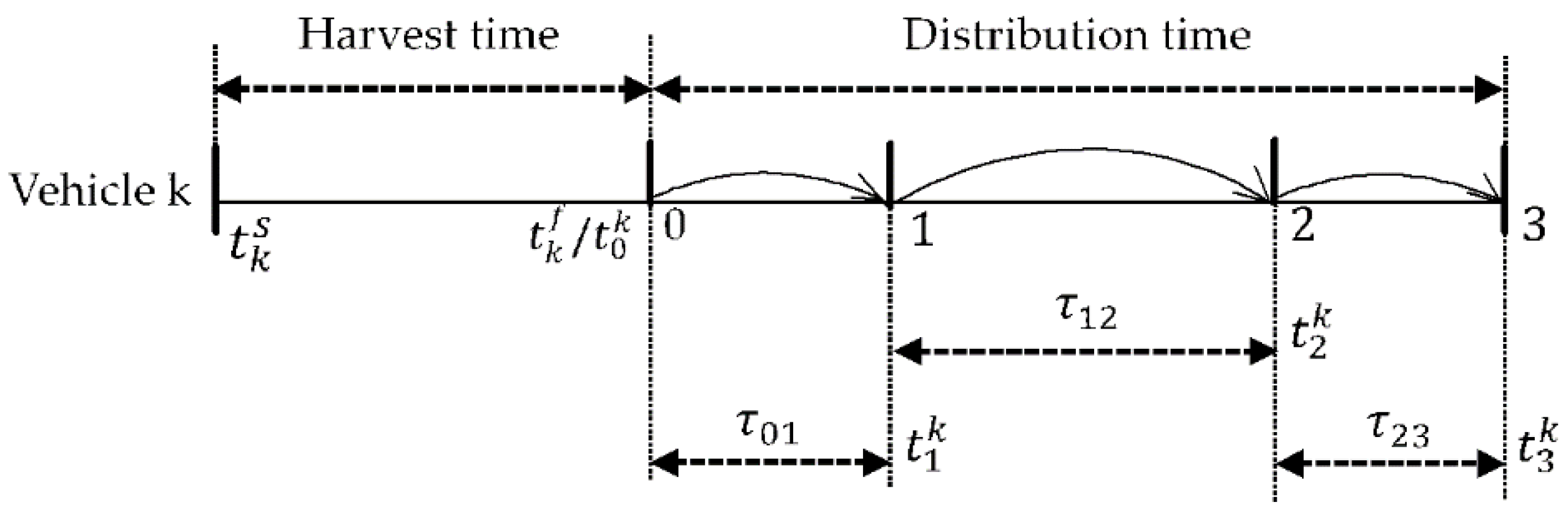
Let denote the time of vehicle arriving at consumers , denote the distribution time from node to node , and denote the starting harvest time and the ending harvest time of perishable agri-products distributed by vehicle respectively, and denote the starting distribution time of vehicle leaving at the harvest location. In this study, we assumed the time gap between the ending harvest time and the starting distribution time, i.e., was equal to . Figure 1 demonstrates the harvest and distribution scheduling process. Vehicle served consumers , , and starting from harvest location . The optimal decision problems focused on what time to do harvest operation, what time the vehicle leaves the harvest location, how many vehicles needed to serve the consumers, and how many consumers are served by the same vehicle and at what optimal sequence. In this study, we aimed to capture and formulate these decision questions.
Note that, for the explanation of parameters and variables used in the proposed model, please refer to Appendix A.
3.2. Objective Function
We considered three different objectives in this study, i.e., the average quality decay cost in the harvest phase, the average quality decay cost in the distribution phase, and the distribution cost.
3.2.1. Average Quality Decay Cost in the Harvest Phase
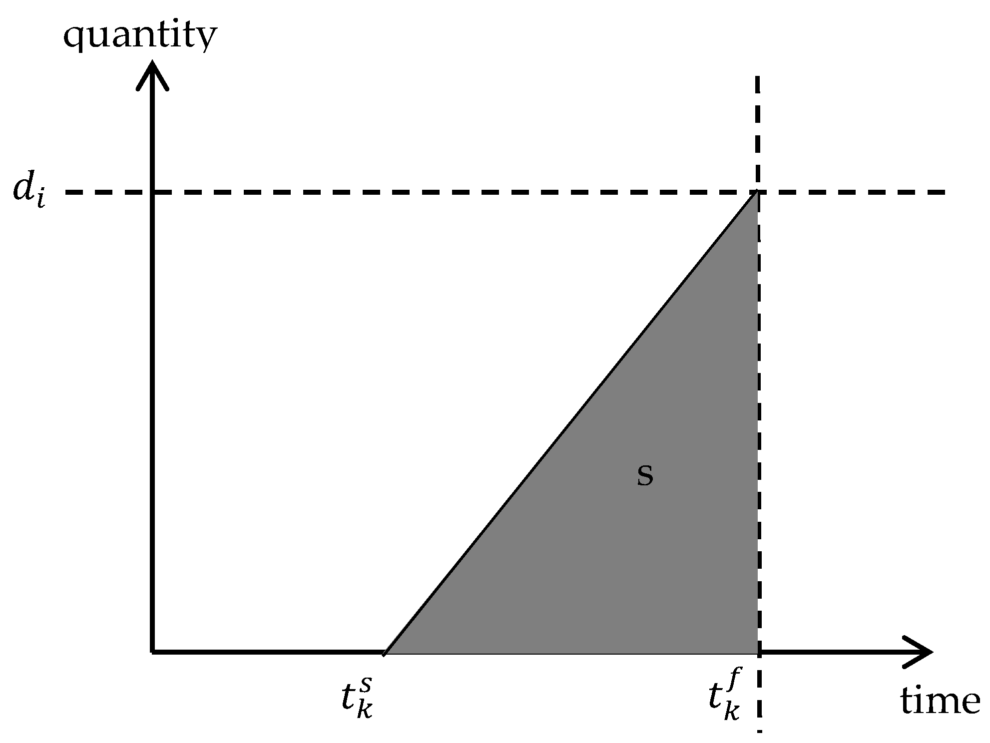
Figure 2 depicts the quantity variation from to , in which denotes the demand of consumer and denotes the shadowed area. In this study, we considered the quality decay of perishable agri-products from the starting harvest time. Let denote the quality decay rate. Inspired by the study in [35], we can calculate the average quality decay from the starting harvest time to the ending harvest time as shown in Figure 2. The average quality decay can be calculated as .
To optimize the quality decay cost during the harvest time period, the key problem focused on how many consumers and their delivery sequence were served by a same vehicle. Therefore, in the harvest phase, the optimal decisions were how much total time was needed to harvest and when to start the harvest operation, so as to meet the time window and demand requirement for each served consumer in the following distribution phase.
Let denote the average quality decay cost in the harvest phase. The calculation is given in Equation (1).
where are continuous decision variables and is a binary decision variable, which equals 1 if the consumer is served by vehicle and otherwise. Therefore, is a nonlinear objective function which could hardly be solved. We adopted the big M method to transform it into a linear model by adding auxiliary decision variables. The big M method is an effective and regular approach used to deal with the nonlinear integer optimization and has been widely adopted to convert nonlinear mixed integer decision variables into a linear one [38]. The formulated function is given in Equation (2).
where and . They are subject to the feasible constraints given in Equation (3).
3.2.2. Average Quality Decay Cost in the Distribution Phase
In this objective, the quality decay cost was calculated from the vehicle leaving time at the harvest location to the arriving time at consumers . Let denote the average quality decay cost in the distribution phase, which can be calculated in Equation (4).
Similarly, is also a nonlinear objective function which can be transformed into an equivalent linear form by using the big M method. Let and . can be rewritten in Equation (5), with the feasible constraints given in Equation (6).
3.2.3. Distribution Cost
This objective contained fixed vehicle cost and distribution cost. Here, is a parameter, and if node , then otherwise . Let denote the unit distribution cost of vehicle , denote the fixed cost of vehicle . is a binary decision variable, taking a value if the arc belongs to the route of vehicle and otherwise. The distribution cost can be calculated in Equation (7).
3.3. Constraints
We formulated the model as an VRPTW problem and constraints are given as follows.
Constraints (8)–(12) were constraints of VRP. Constraints (8) and (9) limited each consumer to be visited by only one vehicle. Constraint (10) was a network flow conservation constraint. Constraints (11) and (12) limited each vehicle departing and returning the harvest location to at most one time. Constraint (13) referred to the vehicle that will serve consumer if it is a node on the corresponding route. Constraint (14) was a constraint of vehicle capacity. Constraint (15) was a constraint of vehicle quantity. Constraint (16) defined the relationship between the starting harvest time and the ending harvest time for vehicle . Constraints (17) and (18) denoted the relationship between finishing harvest time, starting distribution time, and arriving time at consumer . Constraint (19) limited the time of vehicle arriving at consumer . Note that, constraint (19) can eliminate the case of subtours because, if then , otherwise, then Constraints (20) and (21) were constraints on time windows at harvest location and each consumer. Constraint (22) limited as binary decision variables.
3.4. Programming Model
According to the discussions in Section 3.2 and 3.3, the total objective function was to minimize , and by subjecting them to constraints . However, since the magnitude of , and were different, we adopted the Min-Max normalization method to normalize the three objectives in the same magnitude, i.e., .
Therefore, the integrated harvest and distribution scheduling model after normalization can be written as the following:
.
Note that model (23) is a VRPTW problem, which has proved to be an NP-hard problem [39]. If constraints (19), (20), and (21) are removed, model (23) is equivalent to the VRP problem. Moreover, if let , and only one vehicle used, model (23) is equivalent to the travelling salesman problem (TSP). If the vehicle capacity constraint (14) is removed, model (23) can be converted into a multiple traveling salesman problem with time window (m-TSPTW).
4. Numerical Simulation
4.1. Example Setting
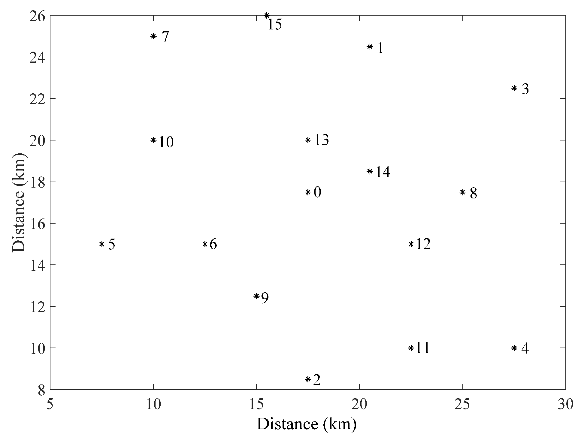
In this example, the logistics network consisted of a harvest location and consumers . The harvest location had six homogeneous vehicles with the average speed of . The harvest location provided one kind of perishable agri-product. The unit harvesting time was for a unit perishable agri-product. The quality decay rate was unit/h. The time window of harvest location was (For simplicity without generality, was assumed as , and was assumed as during the calculation in the example.). Table 1 gives the delivery time between each node located in different geographical locations, in which M denotes an infinite number, which refers to the node pair not being linked geographically. Figure 3 demonstrates the spatial location of each node in the coordinate according to the data given in Solomon’s problem [40]. The coordinate of the harvest location was (17.5, 17.5). Table 2 gives the spatial location, demand, and time windows of each consumer.
4.2. Numerical Results
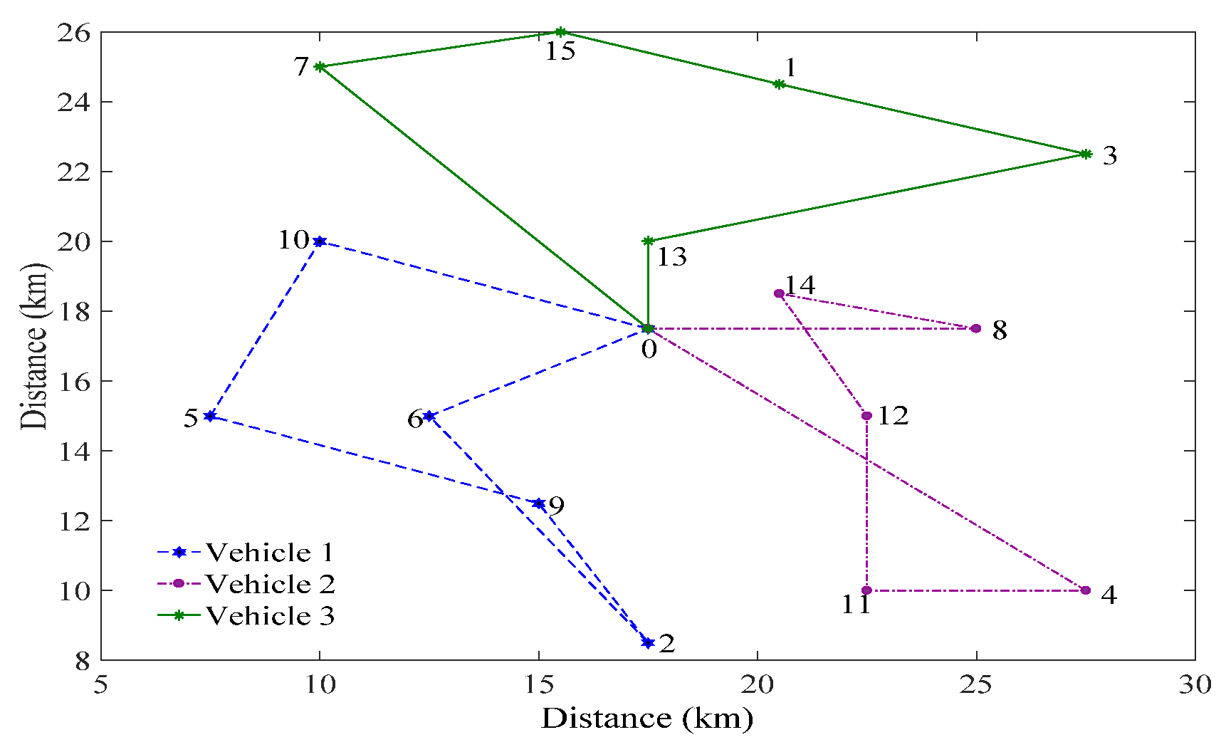
The numerical results are reported in Table 3. It can be seen that the optimal route of vehicle starts from harvest location , and serves the consumers with the sequence , and then returns to harvest location . The optimal starting harvest time for the distribution assignments by vehicle is a.m. Similarly, the optimal route of vehicle is , with the optimal starting harvest time for the distribution assignments by vehicle being a.m. For vehicle , the optimal route is , with the optimal starting harvest time a.m.
According to the results given in Table 3, Figure 4 depicts the optimal vehicle route of vehicle , vehicle , and vehicle . Note that, the optimal vehicle route of vehicle is . It can obviously be seen that the total route length of the optimal route is much longer than the vehicle routing sequence 0. That is because the time window of consumer is earlier than consumer , which constrains vehicle to serve consumer 9 first rather than according to the shortest path. Similarly, the optimal vehicle route of vehicle presents the same phenomena. Therefore, the results given in Table 3 and Figure 4 show that the optimal routes are not the shortest paths due to the impact of time window constraint in the proposed model.
4.3. Sensitivity Analysis
We further carried out sensitivity analysis in terms of different quality decay rate, different time windows, and different number of vehicles.
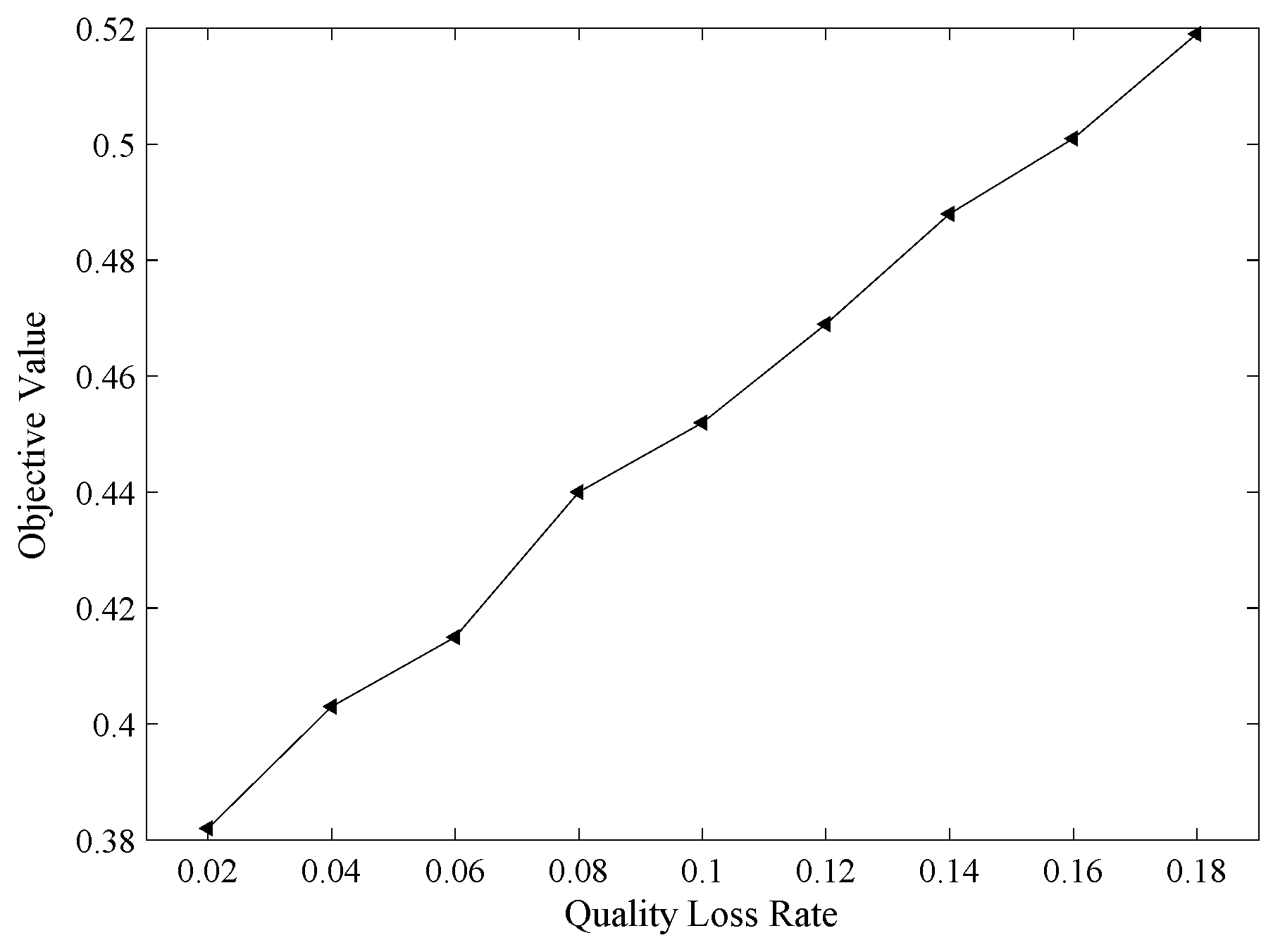
4.3.1. Sensitivity Analysis on Quality Decay Rate
We varied the quality decay rate from to . The numerical results are reported in Table 4 and the objective values are given after normalization. Figure 5 depicts the relationship between the quality decay rate and the model objective value. It can be seen that the objective value is increasing with the growing of the quality decay rate. In other words, if the perishable agri-products has a higher quality decay rate, the harvest location will adopt more vehicles to distribute the perishable agri-products to consumers, so as to maintain the freshness and reduce the deterioration loss.
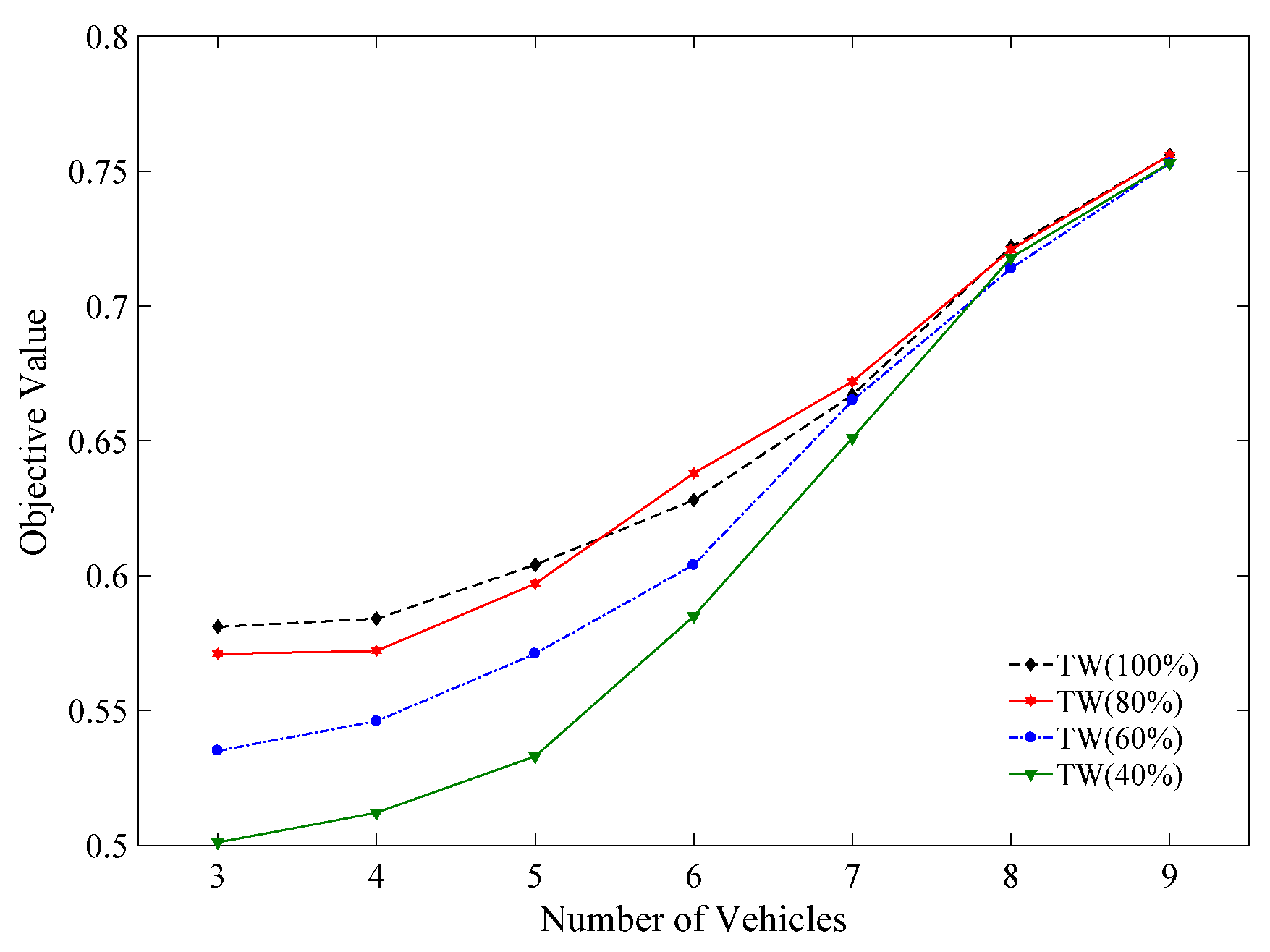
4.3.2. Sensitivity Analysis on Time Windows
We changed the number of vehicles from to and relaxed the time window constraint under four cases, denoted as TW , TW , TW , and TW . TW means that all consumers have time window requirements; TW means that of consumers have time window requirements; TW means that of consumers have time window requirements; and TW means that of consumers have time window requirements. Figure 6 shows that with the increasing number of vehicles, the objective value improves under four cases of TW requirements and is almost approaching the same value if the vehicle number equals nine. We conclude that the objective value will improve rapidly when the vehicle number increases more because of the large proportion of fixed costs in objective value.
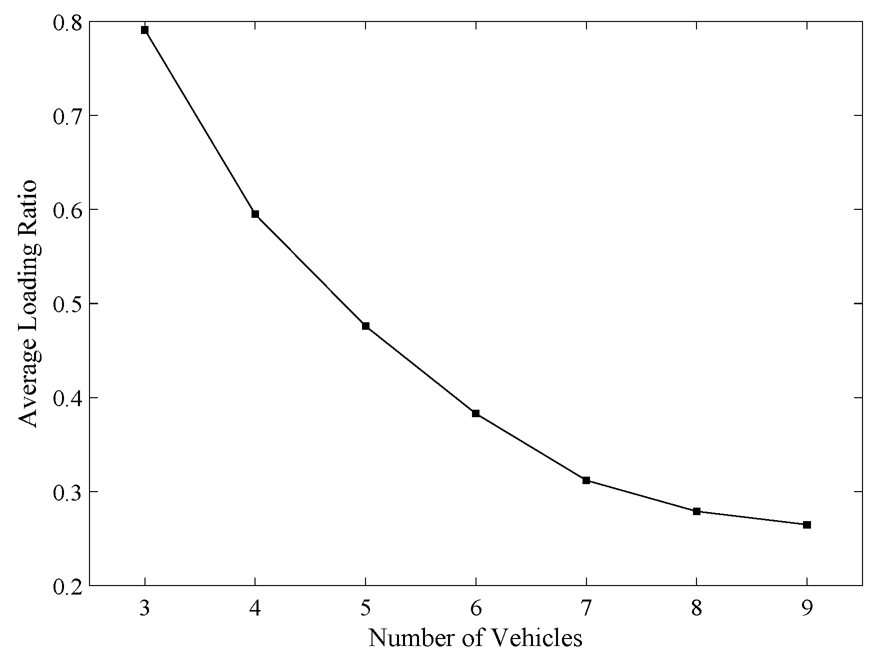
4.3.3. Sensitivity Analysis on Vehicles
We changed the number of the vehicles from three to and calculated the average loading ratio under the time window constraint of each consumer. The average loading ratio refers to the average value of all vehicles’ loading ratio, while the loading ratio equals the total vehicle distributed amount divided by its capacity. Figure 7 depicts the variation trend between the average loading ratio and the number of vehicles. Obviously, with an increasing number of vehicles, the average loading ratio goes down.
According to the above discussions, we can summarize two management insights from this study. On one hand, increasing the number of vehicles could reduce the quality decay of perishable agri-products, and at the same time, it could also lower the average loading ratio and increase the total cost. On the other hand, in order to meet the fresh quality requirement of consumers, the harvest location could increase the number of vehicles to prevent quality deterioration of perishable agri-products.
5. Conclusions
In this study, we have proposed mixed integer nonlinear programming to model the integrated problem of perishable agri-products harvest and distribution scheduling with time windows, with the objectives of minimizing the average quality decay cost and the distribution cost. In the proposed model, we initially proposed an average quality decay function to capture the quality decay of perishable agri-products during the harvest and distribution phases. Therefore, a big M method was adopted to convert the nonlinear objective function into a linear form. In addition, numerical experiments have been conducted to verify the efficiency and effectiveness of the proposed model, and the numerical results and sensitivity analysis have also been reported. Finally, we discussed how the results could serve as a guide for operations management of agri-products in practice.
There are specific areas in this study that can be researched further. This study only considered a single harvest location with a single type of perishable agri-product, hence multiple harvest locations and multiple types of perishable agri-products could be considered as a prospect. Another prospect would consider the penalty cost for time windows in the objective function. Finally, future studies could incorporate more uncertain factors into the integrated harvest and distribution scheduling, such as the uncertainties of consumer demand and time windows, and the uncertainties of temperature and weather condition. We leave these problems for the future work.
Author Contributions
Y.J. conceived and designed the research work; Y.J. and L.C. wrote the paper together. Y.F. checked the expression in English.
Acknowledgments
This research was supported by Natural Science Foundation of Jiangsu Province, China (BK20160742), Humanity and Social Science Youth Foundation of Ministry of Education of China (17YJC630048), Fundamental Research Funds for the Central Universities (NAU: KYZ201663; NAU: SKYC2017007; NAU: SKTS2016038; NAU: SKYZ2017025), High Quality Engineering of Social Science Application Fund in Jiangsu (17SYC-026), and Project of Philosophy and Social Science Research in Colleges and Universities in Jiangsu (2017SJB0030).
Conflicts of Interest
The authors declare no conflict of interest.
Appendix A. Explanations of Parameters and Decision Variables for the Proposed Model
Parameters:
: index of consumers , D;
: index of node ; When is 0, denotes the harvest location.
: index of vehicle ;
: the demand of the consumer ;
: the quality decay of per unit perishable product;
: unit harvest time of the perishable product;
: the unit distribution cost of the vehicle ;
: the fixed cost of vehicle ;
: if then ; otherwise ;
: capacity for each vehicle;
: the distribution time from node ; to node ;
: the time of vehicle arrived at consumer ;
: the ending harvest time of the perishable agri-product distributed by vehicle ;
: binary decision variable, taking a value if the consumer is served by vehicle and otherwise;
[,]: the time window of the distribution center;
[,]: the time window of consumer ;
Decision Variables:
: the starting harvest time of the perishable agri-product distributed by vehicle ;
: binary decision variable, taking a value if the arc belongs to the route of vehicle and otherwise.
References
- Fresh E-Commerce Trade Size in 2016 and Development Trend Prediction Analysis in 2017. Available online: http://www.askci.com/news/hlw/20161205/17582081104.shtml (accessed on 28 February 2018).
- Is the Loss Rate of Fresh Agri-Products in China is 5 Times as High as Developed Countries? Available online: http://www.chyxx.com/research/201801/601051.html (accessed on 28 February 2018).
- Jigang Wei: Why Logistics Costs are High in China? Available online: http://www.sz.gov.cn/szsfzyjzx/jczx/zjgd_1/201707/t20170714_7876798.htm (accessed on 28 February 2018).
- Giri, B.C.; Chakraborty, A.; Maiti, T. Quality and pricing decisions in a two-echelon supply chain under multi-manufacturer competition. Int. J. Adv. Manuf. Technol. 2015, 78, 1927–1941. [Google Scholar] [CrossRef]
- Ghare, P.M. A model for an exponentially decaying inventory. J. Ind. Eng. 1963, 14, 238–243. [Google Scholar]
- Rong, A.; Akkerman, R.; Grunow, M. An optimization approach for managing fresh food quality throughout the supply chain. Int. J. Prod. Econ. 2011, 131, 421–429. [Google Scholar] [CrossRef]
- Wang, X.J.; Li, D. A dynamic product quality evaluation based pricing model for perishable food supply chains. Omega 2012, 40, 906–917. [Google Scholar] [CrossRef]
- Mohapatra, P.; Roy, S. Mathematical model for optimization of perishable resources with uniform decay. Comput. Intell. Data Min. 2015, 23, 447–454. [Google Scholar]
- De Keizer, M.; Akkerman, R.; Grunow, M.; Bloemhof, J.M.; Haijema, R.; van der Vorst, J.G.A.J. Logistics network design for perishable products with heterogeneous quality decay. Eur. J. Oper. Res. 2017, 262, 535–549. [Google Scholar] [CrossRef]
- Nekvapil, F.; Brezestean, I.; Barchewitz, D.; Glamuzina, B.; Chis, V.; Pinzaru, S.C. Citrus fruits freshness assessment using Raman spectroscopy. Food Chem. 2018, 242, 560–567. [Google Scholar] [CrossRef] [PubMed]
- Chen, X.J.; Wu, L.H.; Shan, L.J.; Zang, Q.X. Main factors affecting post-harvest grain loss during the sales process: A survey in nine provinces of china. Sustainability 2018, 10, 661. [Google Scholar] [CrossRef]
- Qin, Y.Y.; Wang, J.J.; Wei, C.M. Joint pricing and inventory control for fresh produce and foods with quality and physical quantity deteriorating simultaneously. Int. J. Prod. Econ. 2014, 152, 42–48. [Google Scholar] [CrossRef]
- Kasso, M.; Bekele, A. Post-harvest loss and quality deterioration of horticultural crops in Dire Dawa Region, Ethiopia. J. Saudi Soc. Agric. Sci. 2018, 17, 88–96. [Google Scholar] [CrossRef]
- Bruckner, S.; Albrecht, A.; Petersen, B.; Kreyenschmidt, J. A predictive shelf life model as a tool for the improvement of quality management in pork and poultry chains. Food Control 2013, 29, 451–460. [Google Scholar] [CrossRef]
- Thuankaewsing, S.; Khamjan, S.; Piewthongngam, K.; Pathumnakul, S. Harvest scheduling algorithm to equalize supplier benefits: A case study from the Thai sugar cane industry. Comput. Electron. Agric. 2015, 110, 42–55. [Google Scholar] [CrossRef]
- Higgins, A.J.; Muchow, R.C.; Rudd, A.V.; Fordb, A.W. Optimising harvest date in sugar production: A case study for the Mossman mill region in Australia: I. Development of operations research model and solution. Field Crop. Res. 1998, 57, 153–162. [Google Scholar] [CrossRef]
- Lamsal, K.; Jones, P.C.; Thomas, B.W. Continuous time scheduling for sugarcane harvest logistics in Louisiana. Int. J. Prod. Res. 2016, 54, 616–627. [Google Scholar] [CrossRef]
- Caixeta-Filho, J.V. Orange harvesting scheduling management: A case study. J. Oper. Res. Soc. 2006, 57, 637–642. [Google Scholar] [CrossRef]
- Supsomboon, S.; Niemsakul, J. A linear programming for sugarcane cultivation and harvest planning with cane survival rate. Agric. Eng. Int. CIGR e-J. 2014, 16, 207–216. [Google Scholar]
- Ferrer, J.C.; Cawley, A.M.; Maturana, S.; Toloza, S.; Vera, J. An optimization approach for scheduling wine grape harvest operations. Int. J. Prod. Econ. 2008, 112, 985–999. [Google Scholar] [CrossRef]
- Arnaout, J.P.M.; Maatouk, M. Optimization of quality and operational costs through improved scheduling of harvest operations. Int. Trans. Oper. Res. 2010, 17, 595–605. [Google Scholar] [CrossRef]
- Jena, S.D.; Poggi, M. Harvest planning in the Brazilian sugar cane industry via mixed integer programming. Eur. J. Oper. Res. 2013, 230, 374–384. [Google Scholar] [CrossRef]
- Accorsi, R.; Gallo, A.; Manzini, R. A climate driven decision-support model for the distribution of perishable products. J. Clean. Prod. 2017, 165, 917–929. [Google Scholar] [CrossRef]
- Kusumastuti, R.D.; van Donk, D.P.; Teunter, R. Crop-related harvesting and processing planning: A review. Int. J. Prod. Econ. 2016, 174, 76–92. [Google Scholar] [CrossRef]
- Mohammed, M.A.; Ghani, M.K.A.; Hamed, R.I.; Mostafa, S.A.; Ahmade, M.S.; Ibrahimb, D.A. Solving vehicle routing problem by using improved genetic algorithm for optimal solution. J. Comput. Sci. 2017, 21, 255–262. [Google Scholar] [CrossRef]
- Wang, X.P.; Wang, M.; Ruan, J.H.; Zhan, H.X. The multi-objective optimization for perishable food distribution route considering temporal-spatial distance. Proced. Comput. Sci. 2016, 96, 1211–1220. [Google Scholar] [CrossRef]
- Zhang, Y.; Chen, X.D. An optimization model for the vehicle routing problem in multi-product frozen food delivery. J. Appl. Res. Technol. 2014, 12, 239–250. [Google Scholar] [CrossRef]
- Hsu, C.I.; Chen, W.T. Optimizing fleet size and delivery scheduling for multi-temperature food distribution. Appl. Math. Model. 2014, 38, 1077–1091. [Google Scholar] [CrossRef]
- Song, B.D.; Ko, Y.D. A vehicle routing problem of both refrigerated-and general-type vehicles for perishable food products delivery. J. Food Eng. 2016, 169, 61–71. [Google Scholar] [CrossRef]
- Rocco, C.D.; Morabito, R. Production and logistics planning in the tomato processing industry: A conceptual scheme and mathematical model. Comput. Electron. Agric. 2016, 127, 763–774. [Google Scholar] [CrossRef]
- Ahumada, O.; Villalobos, J.R.; Mason, A.N. Tactical planning of the production and distribution of fresh agricultural products under uncertainty. Agric. Syst. 2012, 112, 17–26. [Google Scholar] [CrossRef]
- Amorim, P.; Almada-Lobo, B. The impact of food perishability issues in the vehicle routing problem. Comput. Ind. Eng. 2014, 67, 223–233. [Google Scholar] [CrossRef]
- Lamsal, K.; Jones, P.C.; Thomas, B.W. Harvest logistics in agricultural systems with multiple, independent producers and no on-farm storage. Comput. Ind. Eng. 2016, 91, 129–138. [Google Scholar] [CrossRef]
- Ahumada, O.; Villalobos, J.R. Operational model for planning the harvest and distribution of perishable agricultural products. Int. J. Prod. Econ. 2011, 133, 677–687. [Google Scholar] [CrossRef]
- Soto-Silva, W.E.; González-Araya, M.C.; Oliva-Fernández, M.A.; Plà-Aragonés, L.M. Optimizing fresh food logistics for processing: Application for a large Chilean apple supply chain. Comput. Electron. Agric. 2017, 136, 42–57. [Google Scholar] [CrossRef]
- Wu, Y.; Ma, Z.J. Time-dependent production-delivery problem with time windows for perishable foods. Syst. Eng. Theory Pract. 2017, 37, 172–181. (In Chinese) [Google Scholar]
- Chen, H.-K.; Hsueh, C.-F.; Chang, M.-S. Production scheduling and vehicle routing with time windows for perishable food products. Comput. Oper. Res. 2009, 36, 2311–2319. [Google Scholar] [CrossRef]
- Schrijver, A. Theory of Linear and Integer Programming; Wiley: New York, NY, USA, 1998. [Google Scholar]
- Savelsbergh, M.W.P. Local search for routing problem with time windows. Ann. Oper. Res. 1985, 35, 254–265. [Google Scholar] [CrossRef]
- Solomon, M.M. Algorithms for the vehicle routing and scheduling problems with time window constraints. Oper. Res. 1987, 35, 254–265. [Google Scholar] [CrossRef]
Figure 1.
Schematic graph of harvest and distribution scheduling.

Figure 2.
Quantity variation of consumer i during the harvest time period.

Figure 3.
Spatial distribution of each node (km).

Figure 4.
Optimal route of three vehicles.

Figure 5.
Relationship between the quality decay rate and the objective value.

Figure 6.
Objective value under different number of vehicles and time windows.

Figure 7.
The variation trend between average loading ratio and number of vehicles.


Table 1.
Delivery time for the node pairs (h).
| No. | 0 | 1 | 2 | 3 | 4 | 5 | 6 | 7 | 8 | 9 | 10 | 11 | 12 | 13 | 14 | 15 |
|---|---|---|---|---|---|---|---|---|---|---|---|---|---|---|---|---|
| 0 | 0 | 1.3 | 1.5 | 1.8 | 2.1 | 1.7 | 0.8 | 1.8 | 1.2 | 0.9 | 1.3 | 1.5 | 0.9 | 0.4 | 0.5 | 1.5 |
| 1 | 1.3 | 0 | M | 1.2 | M | 2.7 | 2.1 | 1.8 | 1.3 | M | 1.9 | M | 1.6 | 1 | 1 | 0.9 |
| 2 | 1.5 | M | 0 | M | 1.7 | 3 | 1.3 | M | 1.9 | 0.7 | 2.3 | 0.9 | 1.4 | 1.9 | 1.7 | M |
| 3 | 1.8 | 1.2 | M | 0 | 2 | M | M | 2.9 | 0.9 | M | 2.9 | 2.2 | 1.5 | 1.9 | 1.4 | 2.1 |
| 4 | 2.1 | M | 1.7 | 2 | 0 | M | 2.6 | M | 1.3 | 2.1 | M | 0.8 | 1.2 | 2.4 | 1.9 | M |
| 5 | 1.7 | 2.7 | 3 | M | M | 0 | 0.9 | 1.7 | M | 1.4 | 1 | M | 2.5 | 1.8 | 2.2 | M |
| 6 | 0.8 | 2.1 | 1.3 | M | 2.6 | 0.9 | 0 | 1.7 | 2.1 | 0.6 | 0.9 | 1.8 | 1.8 | 1.1 | 1.4 | 1.9 |
| 7 | 1.8 | 1.8 | M | 2.9 | M | 1.7 | 1.7 | 0 | M | 2.3 | 0.8 | M | M | 1.4 | 2 | 0.9 |
| 8 | 1.2 | 1.3 | 1.9 | 0.9 | 1.3 | M | 2.1 | M | 0 | 1.8 | 2.5 | 1.3 | 0.5 | 1.3 | 0.8 | 2.1 |
| 9 | 0.9 | M | 0.7 | M | 2.1 | 1.4 | 0.6 | 2.3 | 1.8 | 0 | 1.5 | 1.3 | 1.3 | 1.3 | 1.3 | M |
| 10 | 1.3 | 1.9 | 2.3 | 2.9 | M | 1 | 0.9 | 0.8 | 2.5 | 1.5 | 0 | M | 2.2 | 1.2 | 1.7 | 1.4 |
| 11 | 1.5 | M | 0.9 | 2.2 | 0.8 | 0.8 | M | 1.8 | M | 1.3 | M | 0 | 0.8 | 1.9 | 1.5 | M |
| 12 | 0.9 | 1.6 | 1.4 | 1.5 | 1.2 | 1.2 | 2.5 | 1.8 | M | 0.5 | 1.3 | 2.2 | 0 | 1.2 | 0.6 | 2.2 |
| 13 | 0.4 | 1 | 1.9 | 1.9 | 2.4 | 1.8 | 1.1 | 1.4 | 1.3 | 1.3 | 1.2 | 1.9 | 1.2 | 0 | 0.6 | 1 |
| 14 | 0.5 | 1 | 1.7 | 1.4 | 1.9 | 2.2 | 1.4 | 2 | 0.8 | 1.3 | 1.7 | 1.5 | 0.6 | 0.6 | 0 | 1.4 |
| 15 | 1.5 | 0.9 | M | 2.1 | M | M | 1.9 | 0.9 | 2.1 | M | 1.4 | M | 2.2 | 1 | 1.4 | 0 |
Table 2.
Demand requirement and time windows of each node.
| Con. No. | Coordinate | Demand | Time Window | Con. No. | Coordinate | Demand | Time Window |
|---|---|---|---|---|---|---|---|
| 1 | (20.5, 24.5) | 15 | [5.5, 8] | 9 | (15, 12.5) | 11 | [5.5, 7.8] |
| 2 | (17.5, 8.5) | 18 | [5.8, 7.9] | 10 | (10, 20) | 13 | [3.7, 7] |
| 3 | (27.5, 22.5) | 30 | [6.2, 9] | 11 | (22.5, 10) | 7 | [4.6, 6.8] |
| 4 | (27.5, 10) | 19 | [2.7, 6] | 12 | (22.5, 15) | 12 | [5.7, 7.2] |
| 5 | (7.5, 15) | 15 | [4.2, 7] | 13 | (17.5, 20) | 19 | [6.2, 8.6] |
| 6 | (12.5, 15) | 20 | [3.2, 8.3] | 14 | (20.5, 18.5) | 10 | [4.7, 6.7] |
| 7 | (10, 25) | 10 | [4.5, 7.1] | 15 | (15.5, 26) | 14 | [3.8, 5] |
| 8 | (25, 17.5) | 25 | [4, 9] |
Note: Consumer number is abbreviated as Con. No.
Table 3.
Distribution routings of each vehicle.
| Vehicle | Distribution Routing | The Starting Harvest Moment |
|---|---|---|
| Vehicle 1 | 01059260 | 8:50 a.m. |
| Vehicle 2 | 0814121140 | 9:44 a.m. |
| Vehicle 3 | 071513130 | 8:14 a.m. |
Table 4.
Objective value for different quality decay rate.
| Quality Decay Rate | 0.02 | 0.04 | 0.06 | 0.08 | 0.10 | 0.12 | 0.14 | 0.16 | 0.18 |
|---|---|---|---|---|---|---|---|---|---|
| Objective Value | 0.382 | 0.403 | 0.415 | 0.44 | 0.452 | 0.469 | 0.488 | 0.501 | 0.519 |
© 2018 by the authors. Licensee MDPI, Basel, Switzerland. This article is an open access article distributed under the terms and conditions of the Creative Commons Attribution (CC BY) license (http://creativecommons.org/licenses/by/4.0/).
Share and Cite
MDPI and ACS Style
Jiang, Y.; Chen, L.; Fang, Y. Integrated Harvest and Distribution Scheduling with Time Windows of Perishable Agri-Products in One-Belt and One-Road Context. Sustainability 2018, 10, 1570. https://doi.org/10.3390/su10051570
AMA Style
Jiang Y, Chen L, Fang Y. Integrated Harvest and Distribution Scheduling with Time Windows of Perishable Agri-Products in One-Belt and One-Road Context. Sustainability. 2018; 10(5):1570. https://doi.org/10.3390/su10051570
Chicago/Turabian StyleJiang, Yiping, Liangqi Chen, and Yan Fang. 2018. "Integrated Harvest and Distribution Scheduling with Time Windows of Perishable Agri-Products in One-Belt and One-Road Context" Sustainability 10, no. 5: 1570. https://doi.org/10.3390/su10051570
Note that from the first issue of 2016, this journal uses article numbers instead of page numbers. See further details here.