Interaction between Industrial Policy and Stock Price Volatility: Evidence from China’s Power Market Reform

Abstract

This paper examines how China’s power market reform influences the stock price volatility of listed power companies. We use the Iterative Cumulative Sums of Squares (ICSS) algorithm to identify structural breakpoints in stock prices, then analyze the characteristics of stock price volatility based on the GARCH model and report the impact of power regulation on stock price fluctuations based on the Autoregressive Distributed Lag (ARDL) model. Using data on power stock price index followed by industrial policy issued between 2006 and 2012, we find that: (1) three structural breaks in China’s power stock price volatility were related to the promulgation of power market reform policies; (2) industrial policies promote the reduction of power stock price fluctuations and its impact on power stock price volatility is consistent in the long run; and (3) the recent policies related to renewable energy do not have a very significant impact on the power stock market.

1. Introduction

When considering the link between investments and policy in China’s power market, China’s energy regulators have been characterized by overlapping jurisdictions. China’s electricity sector consists of a mix of state and locally owned enterprises [1]. The last major structural change occurred in 2002 with the dismantling of the State Power Corporation, resulting in competition in power generation and openness in energy investment. The government requires certain generators to take a certain share in the market, forcing them to sign contracts with end-users or retailers in annual or sometimes monthly forms to compete with each other. However, the electricity sector is not totally liberalized. Only limited competition has been introduced in electricity generation, and retail pricing is still under administrative regulation. The end-users do not have the autonomy to purchase power, and subsidies on power generation interfere with the development of the pricing system [2]. Where the price signal has a limited role in allocating resources and investment, the business decision and profitability of listed power companies will likewise be affected by industrial policy issued during China’s power market reform. Thus, the stock price volatility will in part depend on the nature and extent of market reform, as well as the interaction between power market reform and the stock market.

China started to combine green energy and industrial policy in its power market reform in 2001, signaled by the Tenth Five-Year Plan which included price support scheme for electricity from renewable sources and subsidies in the push for the broader use of greener energy. Total power consumption in China has grown rapidly, especially from 2002 to 2011, during which the average growth rate of power consumption was more than 10%. The rapid growth in energy consumption and heavy reliance on coal have created serious environmental problems, including local air pollution and depletion of water resources. As air pollution caused by “PM (Particulate Matter) 2.5”, or fine particulate matter, has become a social problem, curbs on coal use as well as the expansion of clean energy use are recognized as urgent tasks. China also set the goal of peaking its CO₂ emissions around 2030 in the “Paris Agreement”, which took effect in November 2016. In this agreement, China’s energy policy is responding to these changes in domestic and international circumstances, and therefore, continued political stress was imposed to reduce CO₂ emissions.

The electricity sector provides an attractive context for our study for several reasons. Firstly, at least during the period of our study, there are distinctive groups of listed companies occupying the majority of market share that has been defined by academic scholars, business practitioners, and policymakers. For example, China’s electric power installed capacity was 1.06 billion kilowatts, among which the five major power groups (Huaneng, Datang, Guodian, Huadian, and Zhongdiantou) were 514 million kilowatts. Other central SOEs (such as Sanxia, Huarun, Guokai, Guanghe, Guohe, etc.) and local power groups accounted for 22.5%. The above-mentioned power generation enterprises accounted for 71.41% of the national installed capacity and most of them are listed in power stock price index (PSPI), and the Shanghai A-share Composite Index (SHCI).

Secondly, the industry is characterized by a sustained large-scale investment and steadily increasing demand between 2006 and 2012. As a result, price, capacity, and quality of service varies insignificantly during this period. Robust empirical evidence suggests that power market reform has affected power generation enterprises through electricity generation efficiency and market penetration of renewable energy. The majority of the empirical studies on the power market reform have focused on spillover effect on electricity generation efficiency; spillover on stock price has been understudied. This is unsatisfactory since not only are large sums of capital investment not easily reversible but also power companies face limited government funding supports for capacity expansion. Government funding only accounts for 5.5%. Around 54% of the funds were raised by firms’ own funds and outside investors during our sample period, and the ratio is even higher for established power companies.

Thirdly, China’s government was to spend $1.7 trillion between 2011 and 2015, in the form of investment, assistance for state-owned enterprises and bank loans. The stock price volatility of listed companies provides an opportunity to identify the policy responses to renewable energy industry at the investment level.

Finally, the power industry is heavily regulated, and detailed data on pricing, capacity, and quality is available at the firm level. The power industry has also been the subject of extensive academic research, which provides a benchmark for the current study.

In sum, with a rising demand for power generation, policies on power generation and consumption are likely to have a key bearing on the financial markets. At the same time, sudden structural breaks may affect the dynamics of stock prices. This study aims to investigate the interdependence between China’s stock market and the China’s power market during 2006–2012 (a substantial slowdown in the increase of primary energy consumption since 2012, with year-on-year increase remaining at 1.0% in 2015, and 1.4% in 2016), with careful consideration paid to the possibility of structural shifts in the mean and variance processes. We identify the impact of China’s power market reform on listed power companies’ performances and capacities to attract investment and explore what kind of reforms would be more suitable for China’s power industry development. Therefore, in the following studies, we address two significant issues: characteristics of stock price volatility of the listed power companies with structural breaks; and the impact of power industrial policy reform on stock price volatility.

This paper proceeds as follows. Section 2 reviews the main studies and results regarding structure breaks in the process of stock price fluctuation, and the factors affecting stock price volatility. In Section 3, we discuss the data used as well as variable selection. Section 4 introduces methodologies, including: (1) the iterative cumulative sums of squares (ICSS) method for determining the structure break of stock price volatility; (2) generalized autoregressive conditional heteroskedastic (GARCH) model for analyzing the characteristics of stock price volatility; and (3) autoregressive distributed Lag (ARDL) model for studying the impact of power industrial policy reform on stock price volatility. We present the results and analysis in Section 5 with conclusion and discussion in Section 5.1 and Section 5.2, respectively.

2. Literature Review

Structural break in stock price fluctuation is an active topic. Many studies have attempted to identify the most important event that precipitates structural breaks, such as macroeconomic events, reform policies, and crisis events. Many scholars considered the macroeconomic situation to be the most important factor [2,3]. For example, Chihoun and Mi-Ok found that firms with SEO (Seasoned Equity Offerings) have sustainable development in operational structural change [4]. Fama argued that capital expenses, industrial production, gross national product (GNP), money supply, inflation and interest rates have a strong positive influence on stock price fluctuations [5]. By using the iterated cumulative sums of squares (ICSS) algorithm, Hammoudeh and Li studied the characteristics of stock market volatility in the Arabian Gulf region, and they found that structural changes were usually caused by the impact of international events, for instance, the Asian Financial Crisis. They suggested that international events were the major origins of structural changes [6]. Wang and Tomoe tested stock return data from 1994 to 2006 of five new European Union (EU) members and argued that reform in emerging stock markets, exchange rate policies and the financial crisis led to volatility. They also pointed out that many former studies did not consider the structure of the volatility, which resulted in overestimating volatility [7]. Babikir et al. measured the Johannesburg Stock Exchange All-Share Index and found that structural breaks mainly stem from international financial crises; they argued that the presence of a structural breakpoint should be considered in forecasting stock market volatility, especially in the long term [8].

Significant attention has been paid to the characteristics of fluctuations in China’s stock prices and the influential factors. Chen and Huang (2002) illustrated that asymmetry features existed in fluctuations in China’s stock market, meaning that the impact of negative information on stock price fluctuation was greater than that of positive information [9]. Wang and Zhang indicated that China’s stock market had a long memory consistently, which meant that some unexpected events had a long-lag influence on stock price fluctuations and current risks would affect future risks continuously [10]. There are different opinions about various characteristics across different stages in China’s stock market. Song and Jiang suggested that Chinese stock market volatility had poor stability, and the stratification of stock price volatility was hard to distinguish [11]. Schwert related stock market volatility to the time-varying volatility of a variety of macroeconomic variables, including money growth, industrial production growth, and other measures of economic activity [12]. Wang and Gao concluded that there were weak correlations among the Chinese stock market, inflation, money supply, and stock price volatility [13]. Moreover, Wen et al. argued that there were relationships between oil prices, economic growth, money supply, inflation and Chinese stock market volatility by using data from 2002 to 2010 based on the multi-factor EGARCH (1, 1)-M model [14]. Dong and Wang found a negative relationship between stock market volatility and economic growth in China by using data from 1993 to 2007 based on the Wavelet Transform method [15]. Beltratti illustrated that the stock price volatility of the S&P 500 Index was affected by the volatility of economic and policy variables, and a positive relationship existed between economic growth and price volatility. Of particular interest [16], Li and Fu studied factors affecting China’s power stock price and found that coal prices had a significant impact on power stock price fluctuations since thermal power was the largest share of the power industry in China [17]. Zhao (2016) studied the impact of financial crisis on electricity demand in north China, and found electricity consumption, which affected stock value of electric enterprises and economic growth, was highly correlated [18].

In a study literature on the general economy of power market reforms, Meng (2016) [19] and Mou (2014) [20] analyzed the efficiency of China’s thermal power plants. Mou (2014) found that there were generation efficiency disparities and generation-hour arrangement unfairness across plants [20]. Meng (2016) claimed that reform caused a downshift to the “natural” generation efficiency curve of the thermal power industry [19]. Zhu and Yan et al. (2017) [21] and Zhang (2018) [22] analyzed the impacts of renewable electricity promotion. They found that market reform not only promoted the penetration but also increased the utilization ratio of renewables significantly. Shang and Wei et al. (2016) found that market-oriented reforms decoupled China’s CO₂ emissions from total electricity generation [23].

In summary, although there is significant literature on stock price volatility and its influencing factors, only a few studies deal with the stock price fluctuations of power companies (Li and Fu [17], Teng [24], Ming [25]). In addition, studies on the characteristics of China’s power stock price volatility that consider structural breaks and the impact of power regulation on price volatility are scarce. In the related literature on the general economy of power market reforms, the majority of the empirical studies on the power market reform have focused on companies’ generation efficiency and CO₂ emission, spillover effect on the stock market has been understudied [26,27]. The contributions of this paper are twofold: first, our analysis is one of the few studies that examine the stock price volatility characteristics of listed power companies in China; and, second, we address the relationship between China’s power market reform and the relevant stock price volatility.

3. Materials and Methods

3.1. Data Collection and Variable Selection

The data used in this study can be categorized into two groups: (1) the data on determining the structure breaks of stock price volatility and analyzing the characteristics of stock price volatility, which are based on the daily information; and (2) the data for exploring the impact of power industrial policy on power stock price volatility, which are based on monthly information, since macroeconomic variables are considered, and these macroeconomic data can only be obtained at the monthly level.

The first group of dataset refers to the power stock price index (PSPI) and the Shanghai A-share Composite Index (SHCI), which are collected from the Great Wisdom market software. The sample contains 61 listed power companies in China, whose operation fields include thermal power, hydropower, waste heat generation and so on. The market capitalization of China’s listed power companies is more than 480 billion Yuan, accounting for 3.1% of the total market capitalization in the SHSE and SZSE (according to China Securities Regulatory Commission (CSRC): Industry Classification Results of Listed Companies (2nd Quarter, 2013) and Great Wisdom market software). We selected 30 August 2006–15 November 2012 as our study period, since the PSPI was released beginning from 30 August 2006. We limited our study to ending in October 2012 because of a substantial slowdown in the increase of energy consumption since 2012 (YoY increase drops from 12.8% to 5.5%, remaining at 1.0% in 2015, and 1.4% in 2016). Thus, the assumption of steadily increasing demand is invalid. In addition, a few listed companies seek the development outside of power market. For example, Dongyuan electrical appliances stepped into the chemical industry, HSI Electric purchase nickel mine assets. We believe that this reflects the strategy of traditional power companies actively seeking change under the background of slow growth of energy consumption. Both samples, PSPI and SHCI, are 1510. The second group of dataset contains 75 samples from August 2006 to October 2012.

The explained variable in this study is Power stock price change (PS), which is measured by the stock price index of 61 China’s listed power companies (CLPC) in SHSE and SZSE. We chose the data of the power stock price index at the end date of each month as monthly data. In this study, we took August 2006 as the base (i.e., Month 0). Power stock price is converted to constant price using Consumer Price Index at month level.

The explanatory variable in this study is power industrial policy, which is referred to as policy that caused the structural break of power stock price. Jin and Tang claimed that policy factor was the major reason for market trend from 1992 to 2000 in China [28]. Malik suggested that events, policies or other kinds of events needed to be considered in process of estimating the volatility of the CLPC stock price [29]. We pay more attention to the impact of power industrial policy on the volatility of power stock price. In this study, the explanatory variable only refers to power industrial policies rather than other kinds of events.

The control variables are the following. (1) Coal price (CP): Thermal power is the most important power in China, meaning a large proportion of costs in the power industry are from fuel consumption, and coal price largely affects the CLPC financial situation and stock price volatility. We used the Datong mixed coal prices from the Fenghuang Finance website (http://finance.ifeng.com/) to capture the coal price. Coal price was converted to constant price based on August 2006, using the Producer Price Index at the monthly level. (2) Power generation (PG): Power generation is an important indicator reflecting GDP growth; meanwhile, it has an important impact on power companies’ profits (China’s on-grid tariff is fixed; power companies’ profits depend largely on the amount of power generation). Power generation data were collected from the Hexun Data Center (http://mac.hexun.com/). (3) Fund supply (FS) on the stock market, which is captured by the supply gap between money M1 and M2. The reason is that the scope of M1 includes cash and call deposit while M2 includes cash, call deposit and fixed deposit, the supply difference between money M1 and M2 can represent the fund used to invest in the stock market. The data of M1 and M2 were collected from the website of the People’s Bank of China (http://www.pbc.gov.cn/).

3.2. Research Methodology

3.2.1. Iterative Cumulative Sums of Squares (ICSS) Method

The ICSS algorithm is used to determine the structure breaks of stock price volatility caused by a policy or other significant events. Structural break means a sudden change at an unknown point in the finance time series. The ICSS algorithm is an effective model to test the possibility of structural breaks and to identify the particular time of structural breaks, which was introduced by Inclán and Tiao [30]. In this method, it is assumed that the series we consider presents stationary behavior for some time, and then the variability of error term changes suddenly. It will not change for some time at the new value until another change occurs. Based on the above assumption, Inclán and Tiao [30] defined the following formula:

$$IT={\sup }_k\left|\sqrt{T/2}{D}_k\right|$$

(1)

where $IT$ represents the structure breaks of stock price volatility.

$$D_k=C_k/C_T-k/T,k=1,2,3,\dots ,T$$

(2)

where $C_k$ is the cumulative sum of the squared observation, which is introduced to estimate the change number and the point in time of change. It is expressed as:

$$C_k={\displaystyle {\sum }_{t=1}^k{\epsilon }_t^2}, k=1,2,3,\dots ,T$$

(3)

where ${\epsilon }_t$ is distributed with 0 mean and variance ${\delta }_t^2$.

$${\epsilon }_t=r_t-\mu$$

(4)

where $r_t$ is the returns on a stock index from time $t-1$ to $t$, $t=1,2,3\dots ,T$. $\mu$ is the constant (conditional and unconditional) mean of $p_t$.

$$r_t=100\times \ln (p_t/p_{t-1})$$

(5)

where $p_t$ denotes the value of the stock index at time $t$.

There are sudden changes in the series when the statistic values drift up or down from the threshold, which define the upper and lower bounds for the drifts. The value of the threshold D* is estimated from 10,000 replicates of series of T independent N (0, 1) observations for the desired p = 0.95, following the same procedure introduced by Inclán and Tiao [21]. If the value of IT is bigger than a threshold given, the null hypothesis is rejected, and the value of $k^{\ast }$ is taken as the break date with high probability. Otherwise, the null hypothesis is accepted, indicating that there is no obvious break point.

3.2.2. Generalized Autoregressive Conditional Heteroskedastic (GARCH) Model

Volatility is a very important indicator in economic and financial research, and the GARCH model is widely used in volatility analysis of portfolios, asset pricing and risk management. Predicting the one-period forecast variance based on recent past variances, Engel proposed the Autoregressive Conditional Heteroskedastic (ARCH) model to calculate the volatility of time series [31]. His student, Bollerslev, extended it to embrace more past information; hence, a more concise expression exists in a GARCH model, which hereafter became one of the main volatility models for time series [32]. Hansen and Lunde (2005) argued that GARCH (1, 1) works quite well in estimating volatility of financial returns as compared to more complicated models. In estimating the GARCH model [33], we studied the different types of (p, q) in stock market based on two most commonly used model selection criteria, the Akaike information criterion and the Schwartz Bayesian criterion, and the underlying assumption of the GARCH model. The most commonly used GARCH model for measuring stock market volatility, GARCH (1, 1), is effective and presents a satisfactory explanation. Therefore, we use GARCH (1, 1) to measure volatility.

The GARCH model has been described typically as the GARCH (1, 1) model. It is widely used in studying volatility issues. More discussion can be obtained from Robert Engle (2001). The GARCH (1, 1) model can be expressed below:

$$y_t=\phi x_t+{\epsilon }_t,{\epsilon }_t~N(0,h_t)$$

(6)

$$h_t=\omega +\alpha {\epsilon }_{t-1}^2+\beta h_{t-1},\omega >0,\alpha >0,\beta >0,\alpha +\beta <1$$

(7)

where $y_t$ is the dependent variable, $x_t$ is the explanatory variable, ${\epsilon }_t$ is distributed with mean 0 and unit variance, $h_t$ represents the conditional volatility of $y_t$, $\omega$ is a constant item, and $\alpha +\beta$ indicates the persistence of the GARCH (1, 1) model. Considering the structure change points identified in the variance, the GARCH model is estimated in different sub-samples with sudden changes displaying the persistence of volatility.

3.2.3. Autoregressive Distributed Lag (ARDL) Model

Based on analyzing the characteristics of power stock price volatility, we intend to find how power industrial policy affects stock price volatility. As aforementioned, we argue that the factors affecting the volatility of power stock prices include power industrial policy, power generation, coal price, and money supply. The model for analyzing the impact of power industrial policy on power price volatility, using the natural logarithm of all variables except the dummy variables of power industrial policy, is as follows:

$$\ln P{S}_t={\alpha }_0+{\alpha }_1\ln P{G}_t+{\alpha }_2\ln C{P}_t+{\alpha }_3\ln F{S}_t+{\displaystyle \sum _{i=4}^7{\alpha }_i}{D}_i+{\gamma }_t$$

(8)

where $P{S}_t$ is power stock price return, or power stock price volatility change at time $t$, $P{G}_t$ is power generation, $C{P}_t$ is coal price, and $F{S}_t$ indicates fund supply on the stock market. $D_i$ is the dummy variable representing power industrial policy that is of most interest. The subscript $i$ represents the policy that brings about the ith time of structure break of the power stock price.

To examine the relationship between explanatory variables and the explained variable in the long-term and dynamic change in short-term, we introduced the Bound Co-integration Test developed by Pesaran et al. [34], which is also called the ARDL model. Compared with other single co-integration tests, this method has two advantages: First, under the condition that the variables are I (0) or I (1), a co-integration test can be carried out regardless of whether a same order integration relationship exists between variables; second, it is more suitable for small samples that range from 30 to 80 in the model estimates. The sample size in this study was small, with only 75 observations. For this reason, it is appropriate for using the method. The ARDL model of Equation (8) is as follows:

$$\begin{array}{l}\Delta \ln P{S}_t={\delta }_0+{\delta }_1\ln P{S}_{t-1}+{\delta }_2\ln P{G}_{t-1}+{\delta }_3\ln C{P}_{t-1}+{\delta }_4\ln F{S}_{t-1}+{\displaystyle \sum _{i=5}^8{\delta }_i{D}_i}+{\displaystyle \sum _{i=1}^4{b}_i}\Delta \ln P{S}_{t-i}+\\ {\displaystyle \sum _{i=1}^4{c}_i}\Delta \ln P{G}_{t-i}+{\displaystyle \sum _{i=1}^4{d}_i}\Delta \ln C{P}_{t-i}+{\displaystyle \sum _{i=1}^4{e}_i}\Delta \ln F{S}_{t-i}+{\displaystyle \sum _{i=1}^4{f}_i\Delta D_i}+{\varphi }_t\end{array}$$

(9)

where $\Delta$ means difference, for instance $\Delta \ln P{S}_t=\ln P{S}_t-\ln P{S}_{t-1}$.

The bounds test is based on the F-test or Wald statistics (Dergiades and Tsoulfidis, 2011) [35], and it is the first step in the ARDL approach. Accordingly, the null hypothesis of Equation (5) is that there is no level relationship that exists across variables for the long-term period. That means:

Null hypothesis: $H_0:{\delta }_1={\delta }_2={\delta }_3={\delta }_4\dots ={\delta }_8=0$;

Alternative hypothesis: $H_1:{\delta }_1\ne 0$, or ${\delta }_2\ne 0$, or …… ${\delta }_8\ne 0$.

The above hypotheses are judged by F-statistics of joint significance of ${\delta }_1$, ${\delta }_2$, ${\delta }_3$, ${\delta }_4$, …${\delta }_8$, and the critical value can be obtained. If the estimates of F-statistics are more than the upper bound of the thresholds, the presence is indication of a co-integration relationship between variables in the long-term; if the F-statistics are less than the lower bound of the thresholds, there is no long-term co-integration relationship between variables; and, if the F-statistics are between the upper and lower bounds of the thresholds, whether the long-term co-integration relationship exists between the variables is unknown.

Co-integration is used to identify whether there is a long-term equilibrium relationship between multi-economic variables. The Error Correction Model (ECM) is used to identify the balance between the long-term statistical relationship, and the short-term dynamic relationship.

$$\begin{array}{l}\Delta \ln P{S}_t=\mu +{\displaystyle \sum _{i=1}^4{b}_i\Delta \ln P{S}_{t-i}}+{\displaystyle \sum _{i=1}^4{c}_i\Delta \ln P{G}_{t-i}}+{\displaystyle \sum _{i=1}^4{d}_i\Delta \ln C{P}_{t-i}}+\\ {\displaystyle \sum _{i=1}^4{e}_i\Delta \ln F{S}_{t-i}}+{\displaystyle \sum _{i=1}^4{f}_i\Delta D_i+}\lambda ec{m}_{t-1}+{\epsilon }_t\end{array}$$

(10)

Equation (10) reflects the dynamic relationship between variables and CLPC return in the short-term.

Since causality tests are sensitive to the stationarity of the series, we first study the stationarity properties of the variables based on a unit root test. Unit root testing is used to study the stationarity properties of variables, and it is an essential tool to test the order of integration. In the case where the order is beyond one, the ARDL method becomes invalid. There are a variety of unit root tests, such as augmented Dickey–Fuller (ADF) (Dickey and Fuller [36]), Elliot–Rothenberg–Stock Dickey–Fuller GLS de-trended (DF-GLS) (Elliot et al. [37]), and Phillips–Perron (PP) (Phillips and Perron [38]), among which the ADF test is generally used when there is a small sample volume (Schwert [12]) Several studies including Perron (1997) [39] and Lumsdaine and Papell (1998) [40] have shown that bias in the usual ADF unit root tests is small after endogenously determining the time of structural breaks. Perron (1997) [39] argues that “if one can still reject the unit root hypothesis under such a scenario it must be the case it would be rejected under a less stringent assumption”. The results of the unit root test are shown in

Table 1. Results of ADF unit root test.

Variables	Original			First Difference
	ADF Statistics	Type (c, t, k)	p-Value	ADF Statistics	Type (c, t, k)	p-Value
PS	−4.821	(c, 0, 5)	0.000
PG	−5.183	(c, t, 0)	0.000
CP	2.689	(c, 0, 1)	0.244	6.668	(c, 0, 0)	0.000
FS	−2.503	(c, t, 0)	0.326	−7.511	(c, t, 0)	0.000

Notes: All variables (monthly data) are in logarithmic form, type (c, t, k) represents intercept, trend, lag order; it is marked 0 if the item is not included. The original ADF of PS and PG is statistically significant at 1%; hence, the first difference results are not provided. According to Rushdi et al. [41], the original value of PS, PG and the first difference value of CP and FS can be calculated together.

. Table 1 shows that power stock price ($PS$) and power generation ($PG$) are I (0), while I (1) for coal price ($CP$) and fund supply on the stock market ($FS$), indicating the suitability of an ARDL model. We provide Figure A1 The Original Coal Price (PI) and Figure A2 First Difference to illustrate the degree and nature of variation in the coal price series. The eyeball test also confirms the conclusions above.

4. Results and Discussion

4.1. Structural Breaks of Stock Price Fluctuation

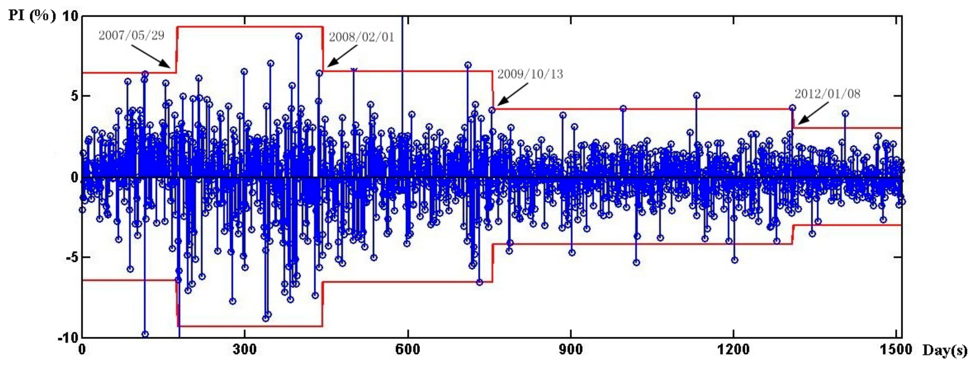
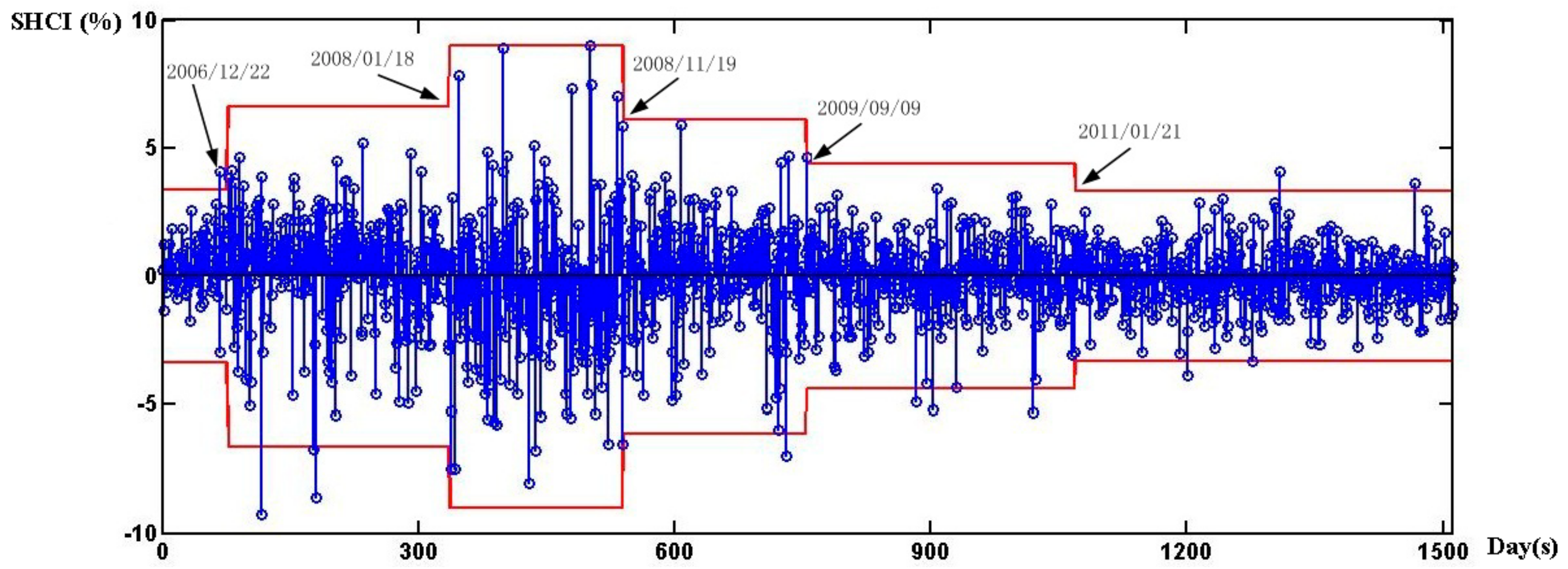
To better illustrate the characteristics of the fluctuation of the Power Stock Price Index (PSPI), we also analyzed structural breaks of the general stock price (Shanghai A-share Composite index: SHCI) and compared the structural break differences between these two stock prices. Results of these structural breaks for PSPI are shown in Figure 1. Results of the structural breaks for SHCI are shown in Figure 2 (the x-coordinate 0 represents 30 August 2006, the x-coordinate 1500 refers to the 1500th day from the start date 0, since the trading day is inconsistent with calendar time). The blue line represents daily return of PSPI. The red line represents ±3 standard deviation bands in different sub-samples. Figure 1 indicates the structure break dates for PSPI are 29 May 2007, 1 February 2008, 13 October 2009, and 18 January 2012, which divide the whole sample into five sub-samples. Figure 2 indicates the structure break dates for SHCI are 22 December 2006, 18 January 2008, 19 November 2008, 9 September 2009, and 21 January 2011, which divide the whole sample into six sub-samples. Based on the results in Figure 1 and Figure 2, a few important findings are made.

Firstly, regarding the frequency of structural breaks, we found that frequency of structural breaks differs between the PSPI (four times) and SHCI (five times), which means that PSPI has experienced fewer structural changes than the SHCI. It also implies that the PSPI is exposed to volatility related to industry events or policy announcements apart from the common elements affecting the general stock market.

$$G_{\max ,n}=\underset{2\le k\le n-2}{\max }{G}_{k,n},G_{k,n}=[(k-1)\ln \left(\frac{{\widehat{\sigma }}^2}{{{\widehat{\sigma }}_1}^2}\right)+(n-k-1)\ln \left(\frac{{\widehat{\sigma }}^2}{{{\widehat{\sigma }}_2}^2}\right)]/C$$

(11)

with

$$C=1+[{(k-1)}^{-1}+{(n-k-1)}^{-1}-{(n-2)}^{-1}]/3$$

(12)

As the analysis is based on the identification of the break dates for the stock prices volatility, a further robust check is needed, given the uncertainty involved in the estimation of the break date. For that reason, we implement the approach proposed by Hawkins and Zamba (2005) [42]. This approach has been recently implemented in economic data by Dergiades et al. (2017) [43]. We follow a similar strategy to examine the in-control hypothesis and monitor changes in variance when the sample is updated with policy shock. We calculate G_max,n statistic based on Equations (11) and (12) and compare it to a critical limit introduced in Hawkins and Zamba (2005) [42]. The results are shown in

Table 2. Gmax and critical value.

	Gmax	h 0.05	h 0.02	h 0.01
D1	29.0692	5.384516	7.323557	8.850193
D2	7.87131	5.419043	7.337222	8.869845
D3	51.1585	5.452387	7.347426	8.884519
D4	32.86207	5.436483	7.342879	8.877981

. G_max,n statistic goes beyond the critical limit at the break dates estimated, which support our hypothesis that variance change may occur when policy announced. The break dates for the stock prices volatility out of control is consistent with what we derive with Iterative Cumulative Sum of Squares approach.

Secondly, from the time perspective of structural breaks, we found that a large difference exists between the PSPI and the SHCI, which means that events in the power industry have a greater impact on fluctuations in the PSPI compared with the macroeconomic environment. The specific date of breakpoints identified by the ICSS algorithm and the corresponding power industrial policies are shown in table.

Table 2 shows that, at the first break point on 29 May 2007, the document of Management of Tariff and Facilities of Desulfurization for Coal-fired Power Units was issued, which implied the operational cost of power generation would increase and the risk of investment in power stock market would increase. As such, the fluctuation of the PSPI increased. At the second breakpoint on 1 February 2008, a policy restricting employees from increasing their share in power generation enterprises was issued. This policy would reduce the flow of funds into the CLPC; hence, the fluctuation of the PSPI took a downward trend. The third break of the PSPI took place on 13 October 2009, when the National Development and Reform Commission and State Electricity Regulatory Commission regulated the power trading price. The policy stipulated that the on-grid power price within a province must be consistent with the standard power price of the province; however, power trading prices across provinces or regions have relative flexibility. The last structure breakpoint is on 13 October 2009, when the State Electricity Regulatory Commission (SERC) issued the document, Drawing the Roadmap for Deepened Reform for Power Development in the Twelfth Five-Year Plan Period. This document stipulates that the industry’s transmission and distribution businesses will be separated into two parts, and large power consumers will be permitted to purchase power directly from power generators; meanwhile, the market will decide the power price. The third and fourth power regulations in Table 2 provided the signal that China’s power market would move in a more orderly and standardized direction, thus decreasing the anticipated risk of investment in this market. Accordingly, the fluctuation of the PSPI decreased.

In addition to the four power regulation policies presented in Table 2, some other important power regulation policies (shown in

Table 3. Structure breaks of China’s power stock price and corresponding policies.

Change Points	Date	Events
1	29 May 2007	Measures of Price and Facility Operation of Desulfurization for Coal-fired Power Units promulgated by the National Development and Reform Commission (NDRC) on 29 May 2007.
2	1 February 2008	Restriction on Employees Increasing Their Share in Power Generation Firms promulgated by State-owned Assets Supervision and Administration Commission of State Council, etc. on 28 January 2008.
3	13 October 2009	Notice on the Regulation of Energy Trading Price promulgated by NDRC and the State Electricity Regulatory Commission (SERC) on 11 October 2009.
4	8 January 2012	Drawing the Roadmap for Deepened Reform for Power Development in the Twelfth Five-Year Plan Period promulgated by the SERC on 08 January 2012.

Source: China Yearbook of Electric Power (2006–2012) [44] and China Electric Power Information (http://www.cpnn.com.cn/).

) were issued over this study period. Distinct from the policies in Table 2, those in

Table 4. Key power regulation policies issued from 30 August 2006 to 15 November 2012.

	Date	Policies
1	13 November 2006	Notice on Promoting the Development of Wind Power Industry issued by the National Development & Reform Commission (NDRC) and the Finance Ministry.
2	20 January 2007	Notice on Speeding up the Work of Shutting Down Small Thermal Power Units issued by NDRC.
3	19 June 2008	Temporary Price Intervention of Coal Used by Power Generation Units issued by NDRC, which provided the highest settlement price of coal.
4	20 July 2009	Notice on Improving Wind Power Price issued by NDRC, which established the benchmark price for different wind power resources.
5	24 July 2011	Notice on Improving Solar Photovoltaic Price issued by NDRC, which established the benchmark price for solar photovoltaic.
6	18 June 2012	Proposals on Encouraging and Guiding Private Capital Flowing into Energy Fields issued by the National Energy Board.

do not contribute to the structural breaks in China’s power stock price. Of the six policies in Table 3, three relate to renewable energy development. Currently, the proportion of renewable energy generation contributes only about 2% of the total power. As such, the policies related to renewable energy do not have a very significant impact on the power stock market.

One in the six policies calls for shutting down small thermal power units. This measure can improve the operating efficiency of power generators; on the other hand, the work itself will increase operational costs in the short run. Hence, it does not have an important impact on power stock price fluctuation.

The policy of price intervention of coal used by power generation units should have an important effect on power stock price fluctuation. However, because it is only a “temporary” price intervention, the effect is not statistically significant.

The most recent policy issued by the National Energy Board on 18 June 2012, is the Proposals on Encouraging and Guiding Private Capital Flowing into Energy Fields. This document stipulated that private investment in energy sectors, such as in power plant construction and industrial upgrading fields, was stimulated. It is beyond any doubt that the introduction of private investment in power fields will promote China’s power industry. However, it is uncertain what impact it will have on China’s listed power firms’ performance. Hence, this policy has no significant effect on the power stock market.

4.2. Analysis of the Fluctuation Characteristics of PSPI

4.2.1. Descriptive Statistics Results

This analysis differs from the previous analysis as the sample is divided into several different sub-samples according to the detected breakpoints obtained by using the ICSS algorithm. Descriptive statistics for different sub-samples are reported in Table 4, which shows that only the mean of the first sub-sample (31 August 2006 to 28 May 2007) is positive. These results indicate that, compared with the period from 31 August 2006 to 28 May 2007, returns on power stock index (or the change of power stock price volatility) decreased from 28 May 2007 to 15 November 2012.

Table 4 also shows that the full sample and all sub-samples are characterized by statistically significant kurtosis (exceeds 3), suggesting that they are leptokurtic, namely demonstrating a fatter tail and a higher peak (the Jarque–Bera test outcome in the sixth column). Meanwhile, the Jarque–Bera result (the sixth column in

Table 5. Descriptive statistics of power stock price volatility.

Sample (Size)	Mean	SD	Skewness	Kurtosis	Jarque–Bera (5) 1	L-B (5) 1
full sample (1510)	0.014	1.887	−0.368	5.839	541.06 *	113.01 *
sub-sample 1 (175)	0.627	2.137	−0.561	5.982	74.03 *	12.393 *
sub-sample 2 (171)	−0.058	2.949	−0.849	4.146	29.887 *	5.71 ***
sub-sample 3 (409)	−0.069	2.514	−0.063	4.348	31.252 *	25.947 *
sub-sample 4 (554)	−0.035	1.392	−0.412	4.152	46.312 *	8.73 ***
sub-sample 5 (201)	−0.028	0.995	0.188	4.341	16.243	3.142

¹ “(5)” means five-order lag. *, **, and *** denote significance at 1%, 5% and 10% level, respectively. There is no ** in the table.

) and Ljung–Box Q-statistic result (the seventh column in Table 4) show that series autocorrelations for squared residuals at any reasonable level exist in the first through fourth sub-samples as well as in the full sample, which indicates that the GARCH model is suitable for these samples except the fifth sample.

The largest standard deviation emerges in the second sub-sample (from 5 May 2007 to 1 February 2008), meaning that, from 5 May 2007 to 1 February 2008, power stock price volatility is the greatest. This volatility occurred during this period because China’s interest rate was adjusted several times; meanwhile, originally non-tradable stocks, such as the stocks owned by state companies, were permitted to be listed and traded.

4.2.2. The Fluctuation Characteristics of the PSPI

Table 6. Results of GARCH (1, 1) model.

Sample (Size)	Coefficients				Variance
	ω	α	β	α + β
full sample (1510)	0.038 *** (0.011) [0.00]	0.059 *** (0.007) [0.00]	0.924 *** (0.008) [0.00]	0.988	3.561
sub-sample 1 (175)	0.007 *** (0.003) [0.00]	0.448 *** (0.126) [0.00]	0.201 (0.189) [0.29]	0.648	4.567
sub-sample 2 (171)	0.002 * (0.001) [0.08]	0.158 * (0.087) [0.08]	0.612 *** (0.179) [0.00]	0.77	8.696
sub-sample 3 (409)	0.004 *** (0.001) [0.00]	0.165 *** (0.051) [0.00]	0.732 *** (0.069) [0.00]	0.897	6.320
sub-sample 4 (554)	0.005 ** (0.003) [0.04]	0.150 *** (0.053) [0.00]	0.600 *** (0.149) [0.00]	0.750	1.938

Notes: ***, **, and * denote significance at the 1%, 5% and 10% levels, respectively. The data in parentheses “( )” are standard deviation; the data in bracket “[]” are p-value.

reports the results of the fluctuation characteristics of the PSPI based on the GARCH model. In terms of the model estimated with the full-sample, the value of $\alpha +\beta$ is the highest with 0.988. The value of $\alpha +\beta$ in sub-series 1 to 4 reduced by 34%, 22%, 9%, and 24%, respectively, compared with the value of the full sample, and the average value decline in sub-samples is 22.75%.

This result shows that power stock price fluctuation persistence stage is reduced typically when considering structural breaks, which is consistent with the conclusions of Kasman [45]. Kasman argued that the value of $\alpha +\beta$ decreased by 29.2% while considering structural breaks. Christopher and William [46], Malik [47], and Rapach and Strauss [48] also stated that, with structure breaks, the persistence of a volatility stage will be reduced.

4.3. The Impact of Power Market Reform on Power Stock Price Volatility

In this section, we first examine the long-term relationship between the variables. We then explore the magnitude of the policy impact on structural changes in the stock volatility. Finally, we examine the policy impact by type.

As previously discussed, to establish a long-term relationship between the variables, an F-test should be applied to Equation (4). The F-test results are displayed in

Table 7. Results of F-test for co-integration.

Explanatory Variables	ARDL-VECM (Lag Order)	F-Statistics	Lower Bound	Upper Bound	Cointegration (Yes or No)
LPG, LCP, LFS	(0, 0, 1)	1.484	2.482	3.757	No
LPG, LCP, LFS, D1, D2, D3, D4	(0, 0, 0, 0, 0, 0, 0)	4.141	2.111	3.363	Yes

Notes: The bound critical value bounds are significant at the 5% level.

. Table 7 shows F statistics are higher than the Upper Bound value when it includes the dummy variable; and the p value is 0.000, indicating that a level of significant co-integration exists between the explanatory variable and the explained variable, as well as between the control variables and the explained variable.

In the search for the optimal length of time for the level variables of coefficients, the lag selection criteria of the Schwarz Bayesian Criterion (SBC) is utilized (Rushdi et al. [41]), and the order of lags is selected as 0. The results in Table 7 imply that a long-term relationship exists between the variables. Then, to estimate the parameters of Equation (5), the ARDL co-integration results between power stock price fluctuations and other variables are reported in

Table 8. ARDL long-run co-integration results.

Variables	Coefficient	SD	T-Statistics	p-Value
LPG	−1.808 **	0.885	−2.043	[0.05]
LCP	−1.131 ***	0.682	−1.659	[0.00]
LFS	2.486 *	0.792	3.140	[0.10]
D1	−0.105	0.391	−0.267	[0.79]
D2	−0.867 **	0.425	−2.039	[0.05]
D3	−1.115 ***	0.442	−2.521	[0.01]
D4	−1.451 ***	0.488	−2.974	[0.00]

***, **, and * denote significance at the 1%, 5% and 10% levels, respectively.

.

Table 8 demonstrates that there is long co-integration between the power stock price (PS) and fund supply (FS), power generation (PG) and coal price (CP). The dummy policy variables (except the first one (D1)) have a significant negative impact on China’s listed power companies’ stock price volatility in the long term. This indicates that China’s power industrial policy reduced the volatility of the power stock price in this study’s period. Market-based regulation is a signal that the power industry will develop toward more orderly operations. Hence, investors have more confidence in the future development of the power industry, and the stability of the power stock market increased. This result is in line with that of Malik [31], who argued that events, such as policy, are important factors affecting the volatility of the CLPC.

Furthermore, we found that the fourth dummy variable—the policy of deepening power market reform promulgated by the SERC—had the greatest impact on volatility. This implies that compared with the policy restricting employees’ investment behavior and reform of the power trading price, reforms affecting the entire power market have greater influences on the power stock market. This result aligns with our expectations: More important policies have a broader influence, and greater impacts will occur.

The co-integration of the control variables, power generation, coal price and stock price is statistically significant, meaning that they have a considerable impact on the power stock market. The negative correlation between power generation (PG) and power stock price indicates that greater the power output is, the lower the PS should be. This finding reveals that macroeconomic growth has a significant negative effect on China’s listed power companies’ (CLCP) stock returns in the long run. This seemingly odd result is caused by the strong speculation that occurs in China’s stock market (Dong and Wang [15]) and is policy-driven (Narayan and Zheng [49]), meaning that policies affect investors’ sentiments more highly than economic growth. Moreover, although China’s economic growth (power generation is an indicator of macroeconomic development) increased quickly in the period of this study, tightening policies during this period—such as raising the deposit reserve rate from 2.25% to 3.50% between 23 December 2008 and 8 June 2012, and strengthening the supervision of the power industry (over this period, more than 10 policies have been implemented to regulate power generators to develop energy savings and environmental protection)—jointly exerted negative impacts on changes in the power stock price.

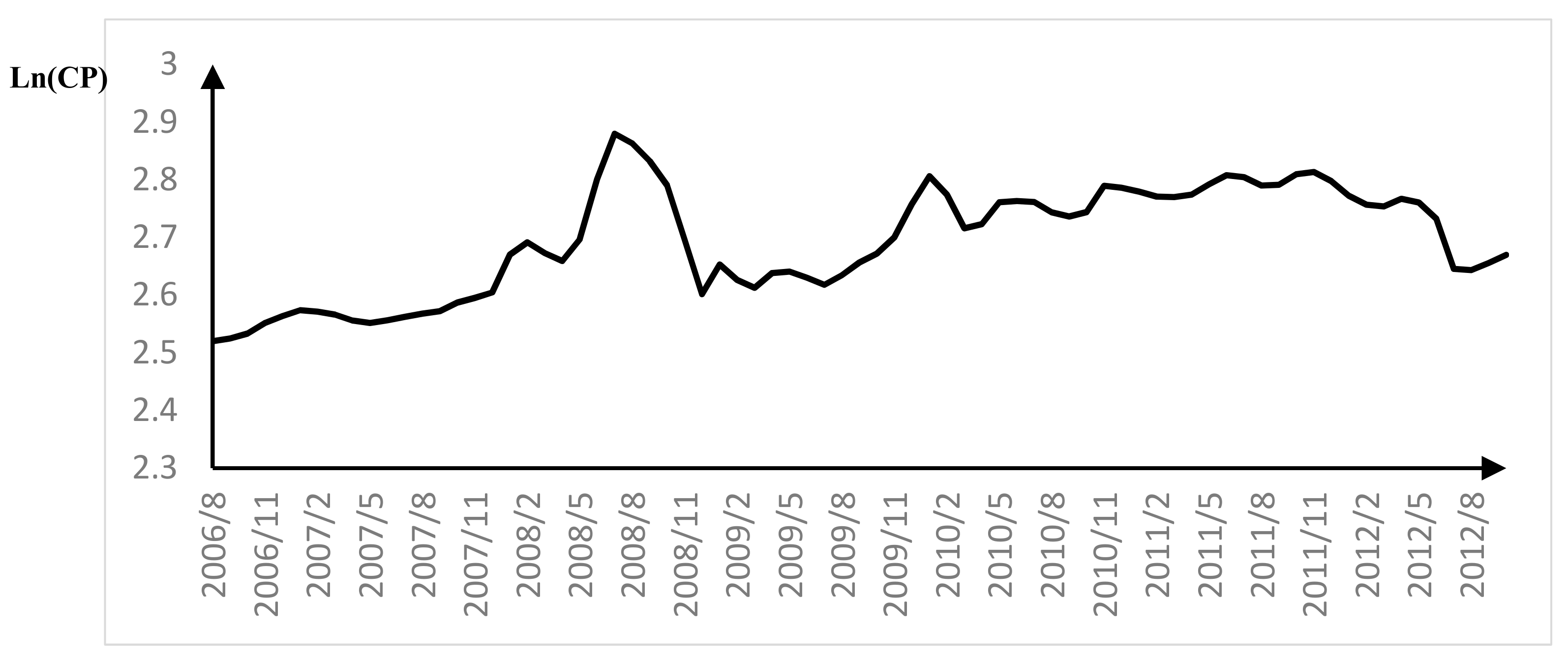
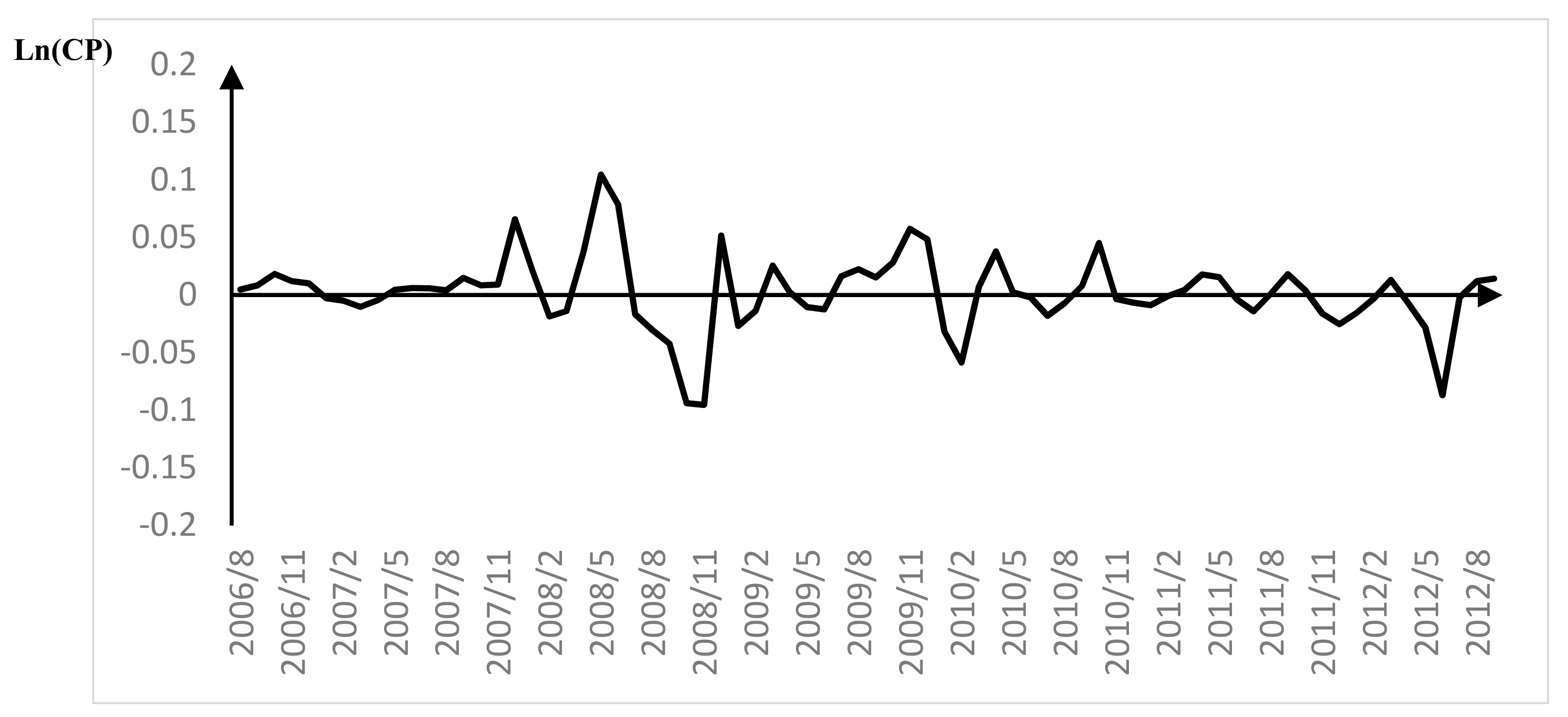
The relationship between coal price (CP) and power stock price fluctuation is statistically significant with a negative value. This means the increase in coal price has a negative impact on power stock price fluctuation; coal price increase caused a decrease in generators’ anticipated profit, and thus reduced the fund flowed into power stock market.

The positive correlation between fund supply on the stock market (FS) and power stock price volatility could be easily understood. Increase in the money supply will lead to additions of money liquidity and nominal wealth; thus, stock prices are more volatile.

The short-run dynamic changes of the relationship between power stock price and other variables (results of ECM) are shown in

Table 9. ECM results.

Variables	Coefficient	SD	T-Statistics	p-Value
∆PG	−0.278 ***	0.108	−2.588	[0.01]
∆CP	−0.174 ***	0.085	−2.236	[0.00]
∆FS	0.383 **	0.110	4.500	[0.03]
D1	−0.157 **	0.073	−2.162	[0.03]
D2	−0.134 ***	0.042	−3.203	[0.00]
D3	−0.172 ***	0.044	−3.905	[0.00]
D4	−0.224 ***	0.049	−4.592	[0.00]
ECM (−1)	−0.154 ***	0.056	−2.741	[0.00]
R-Squared = 0.399 R-Bar-Squared = 0.325			F-Stat. F(7,66) = 6.169 [0.00]

*** and ** denote significance at the 1% and 5% levels, respectively.

. The short-term impact of power market reform on power stock price volatility is similar to that in the long run, which strengthens the result that China’s power market reform reduced the stock price volatility of the listed power companies and the risk of investing in the power stock market. This implies that China’s power market reform favors the expansion of power companies’ ability to attract capital and promote power industrial development.

The only important difference between Table 8 and Table 9 is that the impact of the first policy (D1) on power stock price volatility becomes statistically significant in Table 8. Table 8 also indicates that the impacts of the control variables (PG, CP and FS) are consistent with the results in the long term. The most important difference between short term and long term is that the negative coefficient of dummy variable 1 is statistically significant in a short-run period. This indicates that the policy of Measures of Price and Facility Operation of Desulfurization for Coal-fired Power Units issued by NDRC reduced the fluctuation of power stock price in a short run. This policy aims to encourage coal-fired power firms to invest and operate the facilities of desulfurization. Since this policy is signaled by compulsory administrative characteristics, it affects power stock price only in a short run.

In Table 9, the coefficient of the error correction term is statistically significant at −0.154. This suggests that, when power stock price volatility is above or below its equilibrium level, it adjusts by almost 15.4% within the first year. The results support the notion that with the promulgation of a few power industrial policies, China’s power stock price volatility tended to shrink because these regulations increased investors’ confidence in the orderly development of China’s power market.

The ARDL co-integration approach has certain econometric advantages. It avoids the endogeneity problems and allows researchers to estimate the long-run and short-run parameters of the model simultaneously. However, it is important to stress that the application of the ARDL co-integration technique presumes the existence of a unique long-run relationship among the variables at hand [43,45], a fact quite restrictive for multivariate systems. Towards this direction and as a robustness test for the equilibrium relationship, we also applied the Johansen’s approach via the trace and the maximum eigenvalue tests. The results of the Johansen’s co-integration test on power stock price fluctuations and other variables are reported in

Table 10. Results of the Johansen’s cointegration test.

No. of CE(s)	Trace Test	95% Critical Value	p-Value **	Max-Eigen Value Test	95% Critical Value	p-Value **
None *	84.717	47.856	0.000	45.135	27.584	0.000
At most 1 *	39.582	29.797	0.003	28.355	21.132	0.004
At most 2	11.227	15.495	0.198	10.975	14.265	0.156
At most 3	0.252	3.841	0.616	0.252	3.841	0.616

* Model: Intercept and no trend in cointegration equation and VAR; ** MacKinnon–Haug–Michelis (1999) p-values.

and

Table 11. Results of the Johansen’s cointegration test.

No. of CE(s)	Trace Test	95% Critical Value	p-Value **	Max-Eigen Value Test	95% Critical Value	p-Value **
None *	259.231	159.530	0.000	73.159	52.363	0.000
At most 1 *	186.071	125.615	0.000	50.257	46.231	0.018
At most 2 *	135.814	95.754	0.000	44.674	40.078	0.014
At most 3 *	91.140	69.819	0.000	31.765	33.877	0.088
At most 4 *	59.375	47.856	0.003	28.115	27.584	0.043
At most 5	31.260	29.797	0.034	19.961	21.132	0.072
At most 6	11.300	15.495	0.194	10.987	14.265	0.155
At most 7	0.312	3.841	0.576	0.312	3.841	0.576

* Model: Intercept and no trend in cointegration equation and VAR; ** MacKinnon–Haug–Michelis (1999) p-values.

. The trace test and the maximum eigenvalue test results indicate that there exist two cointegration equations between the explanatory variable and the explained variable, as well as six cointegration equations between the control variables and the explained variable, which is consistent with results in Table 8 and Table 9.

5. Conclusions and Discussion

5.1. Conclusions

Our research controls for possible exogenous shocks in three ways. Firstly, we estimate the effect of various policies along the timeline separately. Using all policy dummy variables in the GARCH model allows us to estimate the coefficient of each policy and observe the scale of policy effect. Secondly, by using the GARCH model, the model incorporates the influence of all past and recent informational shocks on volatility. When we use the policy dummy variables as explanatory variables of volatility, we separate the policy impacts from other effects in the past. Thirdly, we incorporate macroeconomic indicators such as CP, PG, and FS as explanatory variables into the process of estimation. The statistical significance of these economic variables further shows that the Chinese stock price is easily affected by macroeconomic shocks. Considering that macroeconomic factors are not the focus of this study, we do not demonstrate the relevant results for clarity. However, these tests can be regarded as alternative robustness tests.

As one of the important energy-intensive and emission-intensive sectors, China’s power industry has increasingly attracted the attention of researchers and policymakers regarding how to promote more environmentally friendly development. One effective measure to improve energy efficiency is implementing power market reform (Zhao and Ma [50]; Du, et al. [51]; Ma and He [52]). However, the possible negative impact of policies on stock price volatility is a concern for the issue of relative policies.

The main objective of this study was to empirically examine the dynamics of interaction between China’s power market reform and relevant stock price volatility. This paper uses the ICSS algorithm to detect structural breakpoints in power stock price volatility and analyzes volatility characteristics of sub-samples based on the GARCH (1, 1) model. To identify the above result and quantitatively study the impact of power market reform on power stock price volatility, we conduct an ARDL co-integration analysis using relative monthly data from 30 August 2006 to 15 November 2012.

Our results indicate a few broad empirical patterns. We find that, from 30 August 2006 to 15 November 2012, four structural breaks of China’s power stock price volatility occurred, and three of them are related to the promulgation of power market reform policies. In addition, we find that the degree of power stock price fluctuations in each sub-sample decreases with time, indicating that China’s power market reform reduces power stock price fluctuations. These results demonstrate that power industrial policies have a statistically significant negative impact on power stock price volatility, meaning that China’s power industrial policy promote the development of the power stock market by reducing market risks. We give explanations for policies with extreme volatility one by one in Section 5 along with the market conditions at that time. Moreover, Drawing the Roadmap for Deepened Reform for Power Development in the Twelfth Five-Year Plan Period had the most important impact on power stock price volatility in the long-run period with the coefficient of −1.451, and in the short-run period with the coefficient of −0.224. These results indicate that, compared to specific power regulation in Table 3, overall strategic plan for industrial development is more important in terms of degree and scope of influence, thus has a greater impact on the power stock market.

5.2. Recommendation

Industrial policies in the power market aim to not only motivate the investment in renewable energy but also affect company’s value. Therefore, when formulating policies related to investment behavior, the government should focus on the links between different markets. Given our empirical analysis, we provide insights on further design for and implications of industrial policy on the electricity market. At least three implications of this study merit discussion.

Firstly, greater attention should be paid to policies promoting power market reforms in China. Based on our study, few power industrial policies issued between 2006 and 2012 have a significant effect on stock volatility, which implies market reform experience a decade of stagnation. Market-oriented reforms have proven to be beneficial to the stability of China’s power stock market and favorable for power industry development. We hope the new round of power sector reform could make a change.

Secondly, policies promoting the use of renewable energy by subsidizing retailing price and fixed investment is far from satisfactory. Our study indicates the recent policies related to renewable energy do not have a very significant impact on the power stock market. Our findings are consistent with the other scholar’s judgment. Rioux et al. (2017) [53] showed that the increase in the share of renewable energy did not have a significant effect on total generation with coal. A substantial increase in renewables use in China’s energy system would require additional policy interventions.

Thirdly, according to our empirical analysis, the short-term impact of power market reform on power stock price volatility is similar to that in long run, which implies investors have paid considerable attention to the continuing implementation of the policy rather than publish. Therefore, the government should pay attention to clarifying the execution of the policy and providing further detailed information.

5.3. Limitations and Future Research

The paper has a few limitations that present opportunities for future research. First, our analysis is based on data from 30 August 2006 to 15 November 2012, in China. Future studies are required to determine whether the analysis can be expanded to a longer period or wider scope. Meanwhile, in addition to regulation reforms, the difference between detailed policy operation also contribute to the structure breaks of China’s stock price volatility; however, these factors have not been considered in this study.

We offer two speculations about generalizability. On the one hand, SOEs represent particularly strong policy executors that are known to be more aggressive to participate in policy experiments than other companies. The fact that the power market reform triggers different responses from SOEs and private enterprises present important fodder for future research. On the other hand, the power industry is unique in the sense that it is evolving toward deregulation of retailing price and the freedom to invest in renewable energy, which will enhance the profitability of enterprises and achieve dynamic competition in the power industry, in turn, may reduce the interactions between the industrial policy and stock price volatility. However, policies such as limiting the manufacturing development, upgrading the generation equipment, guidance for appropriate investment in thermal power plants continue to have impacts on stock price volatility. In sum, we believe that generalizability is an issue in this study as it is in any single industry study. Replication across industries is necessary before we can attempt to extend the implications of our study to a broader range of industry contexts.

In conclusion, this paper highlights the interaction between industrial policy and stock price volatility. Despite its limitations, it directs our attention to an understudied question in policy-making—how interaction varies within and across the market. We have taken great care to document and explain our methodology to enable replication across industries. We hope this effort spurs more empirical studies of competitive interaction among firms within industries.