Fully Dynamic Input-Output/System Dynamics Modeling for Ecological-Economic System Analysis

Abstract

The complexity of ecological-economic systems significantly reduces our ability to investigate their behavior and propose policies aimed at various environmental and/or economic objectives. Following recent suggestions for integrating nonlinear dynamic modeling with input-output (IO) modeling, we develop a fully dynamic ecological-economic model by integrating IO with system dynamics (SD) for better capturing critical attributes of ecological-economic systems. We also develop and evaluate various scenarios using policy impact and policy sensitivity analyses. The model and analysis are applied to the degradation of fish nursery habitats by industrial harbors in the Seine estuary (Haute-Normandie region, France). The modeling technique, dynamization, and scenarios allow us to show trade-offs between economic and ecological outcomes and evaluate the impacts of restoration scenarios and water quality improvement on the fish population.

1. Introduction

Ecological-economic systems are “undeniably” [1] or even “devilishly” [2] complex. Their complexity and nonlinear dynamic behaviors are due to interactions and feedback between components, processes, and systems [1,3]; non-marginal regimes with multiple equilibria [1]; non-convexity [4,5]; ecological and ecological-economic thresholds [6]; strategic interactions [7]; adaptive processes [6,7]; individual and spatial heterogeneity [7]; and varying time scales and lags [2,7].

This complexity significantly reduces our ability to understand the way ecological-economic systems behave and provide useful policy insights [3,8]. Furthermore, because ecological-economic systems are often viewed as non-separable [1], splitting them in two would be “a poor choice of boundary” [2] and could lead to severe misperceptions, policy failures, and undesirable or counterproductive outcomes [2,7].

Tackling such complexities is only possible via modeling and computer simulations. The ecological-economic model used in this paper captures the complexity of both ecological and economic systems. Practically speaking, dynamic modeling is used to capture the nonlinear feedback dynamics [9]. Recently, integration of such nonlinear dynamic modeling (e.g., SD) with an IO analysis [10,11,12] has been suggested. While dynamic modeling captures the nonlinear dynamics of ecological-economic systems, IO enables the study of sectoral impacts [13,14]. However, there have been few attempts to integrate these two modeling approaches [15,16,17].

Obviously, depending on the type of analysis undertaken, other modeling techniques can be used. For example, if the focus is on individual heterogeneity, an agent-based (AB) model [18] may be preferred to a more aggregate-level dynamic modeling approach such as SD [6,19,20,21]. A hybrid AB-SD model can also be considered [22,23].

Our study develops a fully dynamic ecological-economic model by extending an IO/SD model initially developed by [16] for the ecological-economic system surrounding the Seine estuary. The primary contribution of the previous paper lies in the synchronization of IO and SD, whereas ours is to fully dynamize the model. More specifically, technical coefficients within the IO model will become dynamic along with the relationships between the ecological and economic systems and within the ecological system. Constant technical coefficients have been subject to important criticisms against the use of IO modeling [13]. A fully dynamic ecological-economic model better capturing important nonlinear dynamic behaviors and feedback is in line with a suggestion by [12]. In addition, to capture a qualitative aspect of the ecological system and reflect a critical uncertainty outside the system boundary (i.e., not endogenously determined but externally given in the model), our model adds water quality parameters for the Seine River.

In addition to setting up a model, we also propose scenario developments comprising policy impact and policy sensitivity analyses as methods to examine the model in a more systematic way rather than provide an ad hoc analysis as in [16]. It is another primary contribution of our study.

The remainder of the paper is organized as follows. Section 2 develops the model (IO and SD), details its dynamization, and considers various policy scenarios. Section 3 outlines the results, assesses the impacts of various policies, and undertakes sensitivity analyses. The last section concludes and proposes topics for further study.

2. Materials and Methods

2.1. Study Area

We apply the IO/SD model to the case of degradation of fish nursery habitats by industrial harbors in the Seine estuary (Haute-Normandie region, France). It is well documented that fish nurseries are at risk when harbors develop [24,25]. From 2002–2004, the harbor of Le Havre (Grand Port Maritime du Havre) added 10 km of dykes to extend new infrastructures on the sea to adapt to current worldwide development of huge capacity container ships. The Grand Port Maritime du Havre is the largest harbor in France in terms of container ship traffic, which would have probably been difficult to achieve without the 2002–2004 extension project; and it is France’s second largest harbor for crude oil imports. Upstream in the Seine estuary, the harbor of Rouen is also very important (Europe’s first for cereal exports and France’s second for refined petroleum product transportation). Those two harbors therefore provide a large amount of direct employment and hence, have a critical economic impact in France [26]. Several studies have analyzed ecological impacts of harbors and other human activities on nursery areas in the Seine estuary [16,27,28].

2.2. Model Development

As this is an extension of an earlier model [16], readers interested in the technical details can refer to the previous paper, which also includes the full model description of the SD component in Powersim language in the supplementary information (S4). The model in digital format is also available from the authors upon request. Here we restrict our explanation to the main features of the model and concentrate on its dynamic extension. Following the convention of the SD approach [29], we conduct various model tests as part of the model development (i.e., boundary adequacy, structure assessment, dimensional consistency, extreme condition, integration error, and sensitivity analysis).

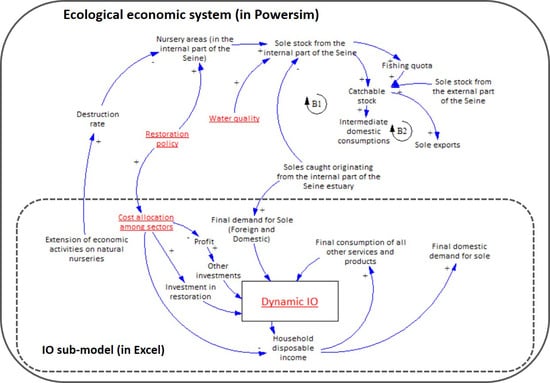
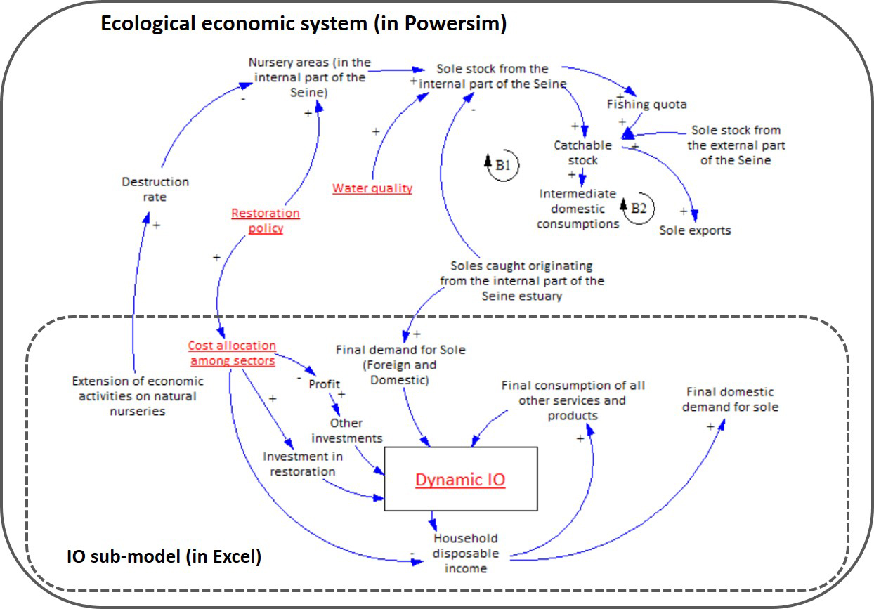
2.2.1. Model Overview

Figure 1 is a simplified representation of how the model captures the ecological-economic system of the study site. It displays the key variables only to highlight the main relationships within the ecological-economic model.

The economic system is embedded in the ecological system as a sub-system. The ecological system is modeled with Powersim (Powersim Studio 10, http://www.powersim.com/), an SD software, and the economic sub-system (IO) is modeled with Microsoft Excel. We integrate the economic sub-system into the ecological system by utilizing Powersim’s function to connect to various datasets, including Excel. The integration is not only capable of transferring data but also allows both Powersim and Excel to run computations internally at each time step of the simulation. Although most economic variables are modeled in Excel (inside the dashed box), some are modeled in SD (Powersim) for technical efficiency.

“Restoration rate” and “Soles caught originating from the internal part of the Seine estuary” are the key variables that connect the ecological system and economic sub-system. Although a higher “Restoration rate” quantitatively improves “Nursery areas (in the internal part of the Seine)”, it incurs a “Cost of environmental measures”. “Soles caught originating from the internal part of the Seine estuary” involves various feedback loops that are a source of nonlinear dynamics of the model. B1 and B2 stand for negative or balancing feedback loops [29]. For instance, a larger “Sole stock from the internal part of the Seine” increases “Catchable stock”, which results in larger “Intermediate domestic consumptions” that drives more “Soles caught originating from the internal part of the Seine estuary”. This increase, however, dampens “Sole stock from the internal part of the Seine”, and so on. “Soles caught originating from the internal part of the Seine estuary” involves other feedback loops such as that of “Dynamic IO”. It is, however, not clear whether the feedback is positive or negative because the impacts of “Final demand for Sole (Foreign and Domestic)” on IO are mixed.

We added “Water quality” as part of the system because of its significance, which is later discussed. It is, however, exogenously given without a feedback relationship in the model because the dynamics and effort of water quality improvement are outside the boundary of the ecological-economic system in the study site (a large part of the contamination in the Seine estuary comes from the city of Paris located at 350 km upstream).

2.2.2. Input-Output (IO) Modeling: The Economic Sub-System

2.2.2.1. Base IO Table

Cordier et al. [16] used the commodity-by-industry IO table for the study area (Haute-Normandie region) comprising 12 commodities and 12 industries for 2007, whereas this paper uses the industry-by-industry IO table for the same area comprising 37 sectors for 2012. Since the regional table does not exist, we construct it for the area studied using the 2010 French national table [30], update data to 2012, and regionalize the table with techniques developed by Jackson [31], Lahr [32], and McDonald [33].

There are several reasons for using industry-by-industry IO tables and 37 sectors. First, detailed sectors allow more precise (sectoral) policy analyses. Second, regionalization of the industry-by-industry IO table is more robust and less time consuming than that of the commodity-by-industry IO table. Finally, the calculation of technical coefficients in regionalized industry-by-industry IO tables can help avoid inconsistencies (i.e., negative values of coefficients) that may occur with commodity-by-industry IO tables.

The IO table (

Table 1. Industry-by-industry IO table [14].

	Buying Sector $\left(\mathit{j}=1,\dots ,\mathit{n};\mathit{n}=37\right)$	Final Demand $\left(\mathit{k}=1,\dots ,\mathit{f};\mathit{f}=8\right)$	Total Output
Selling Sector $\left(i=1,\dots ,n;n=37\right)$	$X$	$F$	$x$
	$x_{ij}$	$f_{ik}$	$x_i$
Imports	$mi\prime$	$mf\prime$	$m$
	$m{i}_j$	$m{f}_k$
Value Added $\left(l=1,\dots ,p;p=3\right)$	$V$ ${\nu }_{lj}$		$v$ ${\mathrm{v}}_l$
Total Outlays	$x\prime$ $x_j$

) comprises three matrices—$X$, the intermediate sales matrix; $F$, the final demand matrix; and $V$, the value added payments matrix—five vectors—$x$, $x\prime$, $v$, $mi\prime$, $mf\prime$, representing total industry output, its transpose, total value added payments, a row vector of imports consumed by industries, and a row vector of imports consumed as final demand—and one scalar $m$ for total imports. The time notation (t) is suppressed when it is not necessary.

We can derive the following relationship from the industry-by-industry IO table (Table 1), which calculates sectoral output ($x$) based on static technical coefficients:

$$x={\left(I-A\right)}^{-1}f=Lf$$

(1)

$I$ and $i$ are respectively an identity matrix and column vector of 1’s known as a summation vector; $f=Fi$; ${\left(I-A\right)}^{-1}$ is renamed $L$ for conciseness and known as the Leontief inverse or total requirement matrix; and $A$ is the matrix of technical (or IO, or direct input) coefficients made of elements $a_{ij}=x_{ij}/x_j=x_{ij}/x_i$ [14]. Equation (1) calculates the direct and indirect impacts of changes in the final demand ($F$) on the industry outputs ($x$). The calculations of the final demand for each sector follow [16] with three adaptations.

First, the final domestic demand for sole is calculated separately from the demand for the 36 other sectors i to relate sole consumption to environmental conditions and measures. The final domestic demand for sole is calculated in tons in the economic sub-system as follows:

$${\left(f_{i=sole,1}^t\right)}^{tons}={\left(f_{i=sole,1}^{t-1}\right)}^{tons}\left(1+e_{i=sole}\frac{Y^t-Y^{t-1}}{Y^{t-1}}\right)$$

(2)

where ${\left(f_{i=sole,1}^t\right)}^{tons}$ enters the SD model and depends on the income elasticity (The income elasticities are adopted from Gohin [34].) ($e_i$) as well as on changes in household disposable income ($Y^t$) from $t-1$ to $t$, which in turn is a function of the cost of environmental measures (${\psi }_i^t$) paid by industries.

Second, the cost of restoration is allocated among economic sectors as follows. The investment ($k=4$) is defined as

$$f_{i,4}^t=\left({\displaystyle \sum }_{j=1}^n{\mu }_j{x}_j^{t-1}-{\left(\frac{1}{2}{\psi }^{t-1}{\alpha }_j\right)}_{inv}\right){\widehat{cap}}_i+{\psi }_i^t,i=1,\dots ,m$$

(3)

where ${{\displaystyle \sum }}_{j=1}^n{\mu }_j{x}_j^{t-1}-{\left(\frac{1}{2}{\psi }^{t-1}{\alpha }_j\right)}_{inv}$ is the total amount of the gross operating surplus used for investment (other than investments in nursery restoration), ${\mu }_j$ is the fixed coefficient of the share of gross operating surplus of sector j used for investment in the output of sector j at the reference year, ${\left(\frac{1}{2}{\psi }^{t-1}{\alpha }_j\right)}_{inv}$ is the part of the total annual restoration cost paid by sector j through a reduction of the part of its gross operating surplus that would have been used for non-restoration investments otherwise, ${\psi }^t$ is the total annual restoration cost at time $t$, ${\psi }_i^t$ is the restoration cost paid at time t by other sectors to sector $i=18$ (the construction sector) to build infrastructures required for nursery restoration; ${\psi }_i^t=0$ for $i\ne 18$, ${\alpha }_j$ is the share of the total annual restoration cost paid by sector j, and ${\widehat{cap}}_i$ is the fixed capital formation coefficient calculated in the IO table at the reference year as the ratio of investment in sector $i$ on total gross operating surplus used for investment.

The third point worth mentioning here is that the sectoral output $x_j^{t-1}$ is not calculated via Equation (1) as in most IO modeling publications. Next, Section 2.2.2.2 explains how we dynamize $x_j^{t-1}$ using Equation (7). This allows us to increase the dynamic property of the equations.

In the scenario development detailed next, we set two cost allocation rules by changing the combination of ${\alpha }_j$.

2.2.2.2. Dynamization of the IO Table

Changes in output $\Delta x$ caused by changes in final demand $\Delta \mathrm{f}$ are expressed as:

$$\Delta x=L{f}^1-L{f}^0=L\Delta f={\left(I-A\right)}^{-1}\Delta f$$

(4)

If constant technical coefficients could be a reasonable assumption for a short-term period (~5–10 years), it is much less so in the longer term. To overcome this issue, several approaches have been proposed [35]) and we use a classical method adopted in various IO-EC models [13,35,36,37].

The key idea is to capture the difference between expected and actual output. To do that, we need to differentiate sectoral output $x$ from Table 1 in two types: (1) the expected (or predicted) output, a vector of sectoral expected output $z_i$ (vector $z$) that is conditional on the base year IO table and, hence, contains the deterministic structure of this table (i.e., ${\mathrm{x}}_{ij}$ values in Table 1, which do not change over time); and (2) the actual output, a vector of sectoral actual output $x_i$ ($x$) that is the historical or forecasted value and expressed as a function of constant price expected output ($z$). Please note that in dynamic IO-EC models, $x$ is a vector of historical sectoral outputs at the stage the model is being built, that is, when modelers use observed time series data to build up statistical regressions that compute $x$ in the current year (time t) as a function of the difference in the previous year (time t − 1) between observed (also named actual) values of $x$ and values estimated (also named expected) by a static IO model. However, once the building stage is completed, the dynamic IO model can be run for forecasting to simulate future sectoral outputs $x$. This is why $x$ is considered a historical (observed) value at the building stage and a forecasted value for forecasting purposes. The term “forecasted” is voluntarily used here to make it clear that it includes dynamic changes in the structure of the economy, which is not the case when we use the terms “estimated” or “expected.”

Both sectoral outputs $z$ and $x$ are computed at the constant price. Unless otherwise mentioned, all prices in this paper are expressed in 2012 Euros. Following Kim et al. [13] and Israilevich et al. [37,38], $z$ and $x$ are expressed as follows:

$$z=Ax+f$$

(5)

$$x=f\left(z\right)$$

(6)

$A$ is a matrix of constant technical coefficients, which is taken from the base year; $f$ is the final demand vector; and $z$ is identical to $x$ in the base year for which technical coefficients (i.e., $A$) are known but then generally differs from $x$ over time as coefficients change.

The Equation (6) relationship can be rewritten as (see [37,38] for detailed description; $f$ in Equation (6) represents the general symbol for mathematical functions, not to be confused with the final demand vector $f$.):

$$x_t=[{(I-{\widehat{\beta }}_{t}A)}^{-1}{\widehat{\beta }}_t]f_t$$

(7)

where ${\widehat{\beta }}_t$ is a diagonal matrix with the elements ${\widehat{\beta }}_{i,t}$, computed as:

$${\widehat{\beta }}_{i,t}=\exp \left[{\alpha }_0+{\alpha }_z\log \left(\frac{x_{i,t-1}}{z_{i,t-1}}\right)+{\alpha }_g{g}_{i,t}\right]\forall i=1,\dots ,n$$

(8)

This transforms the static IO equation into a dynamically determined relationship. The coefficients for ${\widehat{\beta }}_{i,t}$ (${\alpha }_0,{\alpha }_z\mathrm{and}{\alpha }_g$) are estimated using generalized least squares (GLS) to correct for first-order autocorrelation in the residuals in Equation (8) based on historical values (i.e., time series of observed data for $x_t$, $f_t$, and $A$) and on $z_{i,t-1}$ computed in Equation (5).

$$\log \left(\frac{x_{i,t}}{z_{i,t}}\right)={\alpha }_0+{\alpha }_z\log \left(\frac{x_{i,t-1}}{z_{i,t-1}}\right)+{\alpha }_g{g}_{i,t}+{\epsilon }_{i,t}$$

(9)

$g_{i,t}$ is the set of exogenous explanatory variables selected by the modeler, which vary across $i$ (e.g., sectoral value added, gross domestic product (GDP), or employment) and $z_{i,t-1}$ is a lagged input-output-generated predicted output. Equation (9) explains the difference between the actual output ($x_{i,t}$) and the expected output ($z_{i,t}$) (ratio on the equation’s left side) as a function of the ratio of actual and expected outputs of the previous period ($\frac{x_{i,t-1}}{z_{i,t-1}}$), exogenous variables ($g_{i,t}$), and a stochastic component, ${\epsilon }_{i,t}$. In other words, Equations (6) and (7) capture overall changes in technical coefficients over time.

Figure 2 shows overall changes in technical coefficients (i.e., the share of an intermediate input, $x_{ij}$, consumed by a sector $j$ in its total input consumption, $x_j$) from 2012 to 2032. The changes are calculated by subtracting the value of technical coefficients in the reference year 2012 (also called the base year) from their value in 2032. Values for the reference year 2012 are obtained through the regionalization technique of the national IO table as mentioned previously. Technical coefficients for 2032 are estimated using dynamization.

In line with the findings from a similar study on the Chicago metropolitan region by [38], changes are modest (mean: −0.0001; standard deviation: 0.0121). Dark- and light-colored cells respectively show positive and negative changes from 2012–2032. To highlight the changes, we set cells with very little change (i.e., absolute value of changes smaller than 10⁻¹⁷) in white, along with cells in which no change occurs.

Negative changes are dominant in the top left industries of Figure 2 (cells from columns and rows 1 to 18). This suggests that our dynamization equation of technical coefficients succeeds in capturing the current trend of progressive greater degrees of replacement of French industries by those located in developing and emergent countries in which labor costs are much lower (China, central and Eastern Europe, Brazil, etc.). This is particularly the case on the diagonal showing self-consumption within the same sector. For instance, regarding the cell in row 5 and column 5 describing self-consumption within the “wood, paper, printing” sector, the decline is likely because the paper industry (in column 5) is importing ever more wood and paper pulp (from row 5) from Brazil and other emergent and developing countries, as suggested in time series statistics from FBCA [39], Copacel [40], and INSEE [41].

Positive changes are dominant in the bottom right industries of Figure 2 (cells from columns and rows 22 to 37). This suggests that the dynamic technical coefficients reflect the current trend of the increasing rate of services consumption by other service sectors. For example, most service sectors have increased their share of intermediate inputs supplied by sector 30, “rental and leasing activities, etc.” (which also includes many other services to companies and businesses such as interim employment assistance; travel agencies and reservation services; building services, etc.). This also suggests that the dynamization equation of technical coefficients captures the increasing importance of the functionality economy with respect to the conventional economy. That is, industries today prefer renting their equipment to buying them (e.g., car leasing, photocopy renting, computer leasing, etc.) or subcontracting services to other companies rather than supplying them on their own.

2.2.3. System Dynamics (SD) Modeling: The Ecological System

Figure 3 depicts the SD part of the IO/SD model in a stock and flow diagram. The model has two stocks: “Nursery areas” and “Sole stock from the internal part of the Seine.” The nursery areas include 21 categories with different sole abundance to represent the spatial heterogeneities; the categorization is based on the sediment type—gravel, sand, or silt—and the depth. These areas are assumed to be independent, as we do not know how they interact with each other. Another simplification of the ecological model stands with the fact that we do not develop the physical, chemical, and biological conditions required by soles to reproduce, e.g., the spawn is performed in the bottoms where soles inhabit and therefore depends on environmental conditions such as water temperature and acidity, water quality and food availability [42]. The sole stock uses a cohort structure, ages 1 through 10.

The connection between SD and the economic sub-system is represented by bold arrows. Such an arrow leaving a circle (hence, leaving an auxiliary variable) means that the value of that variable is transferred to the economic sub-system. In addition, by correspondence, a bold arrow entering the circle means the value is transferred from the economic sub-system to the ecological system.

Based on Cordier et al.’s [16] work, we update parameter values and add two new components: varying restoration schedule and water quality.

First, concerning water quality, its improvement reflects the qualitative aspect of the nursery. The degradation of water quality is a major anthropogenic disturbance to soles in the Seine estuary [25]. Using the backward predictive approach, Rochette et al. [25] estimated that the juvenile density in the Seine estuary is approximately 23% lower today compared to 1850, primarily because of water quality degradation. Consequently, we assume that water quality improvement can recover the juvenile abundance by 23% maximum as:

$$AbundanceMultiplie{r}_i=WaterQualityIndex\ast AbundanceMultiplie{r}_i^{max}$$

(10)

where Water Quality Index: [0.50, 1.00].

Here, we simply assume that the juvenile abundance is proportional to water quality by conducting a sensitivity analysis. The current (or business as usual) Water Quality Index is set at 0.77 (=100–23%). Further improvement could be expected, as the water quality of the Seine River has shown significant improvements regarding phosphate and ammonium pollution since 2000, when the European Water Framework Directive came into force [43]. However, those authors also point out that water quality is decreasing regarding nitrate pollution. Therefore, we set the plausible range of Water Quality Index to [0.50, 1.00], following Sterman’s [29] warning not to be overconfident about uncertainty and therefore to include a relatively wide range. Our estimation of water quality seems sufficient for this type of analysis but hydrodynamics of water, flow, velocity, … have not been considered here and may potentially impact the analysis).

Second, concerning restoration schedules, we try to explore the impacts of the timing of restoration. Assuming restoration evolves at a constant rate for 10 years from 2013, to meet a predetermined target at the end date, restoration at time $t$ is obtained from:

$$Restoratio{n}^t=\frac{Targetrestoration-10b}{100}\left(2t-t_{-1}-t_0\right)+b,b\in \left[0,5\right]$$

(11)

where $t_{-1}$, $t_0$, and $b$ are a year before the beginning of the restoration, the year the restoration begins, and a parameter determining the speed of restoration, respectively (see S3 for the derivation process). For example, when $b=0$ (Figure 4a), restoration per year increases as time passes. When $b=5$ (Figure 4c), restoration decreases linearly over time. In all cases, however, the same amount of nursery (i.e., Target restoration) is restored at the end of the 10-year period.

2.3. Scenario Development

As suggested by the Millennium Ecosystem Assessment [44], we develop scenarios to explore the complex ecological-economic system, inform planning and decision-making processes, and help bridge the gap between scientific understanding and policy needs.

Our scenarios combine two approaches: policy impact assessment and policy sensitivity analysis. Policy impact assessments examine the economic, social, and environmental impacts of public policy (e.g., OECD [45] and the European Commission [46] and are frequently used in IO [14]. Policy sensitivity analysis is one of the three sensitivity analyses proposed in SD [29]. It tests if policy implications change when assumptions about the model (e.g., parameters with uncertainty) vary over a plausible range [29].

As illustrated in

Table 2. Scenario development specifications.

	Policy Impact Assessment		Policy Sensitivity Analysis	Outcome Indicators (Dynamics and Cumulative Values)
	Restoration Schedule	Cost Allocation	Water Quality
Business as usual (BAU)	no restoration		0.77	Economic outcome indicators 1. GDP (M€) 2. Disposable income (M€) 3. Gross operating surplus (GOS) (M€) Ecological outcome indicators 4. Soles caught (originating from the internal part of the Seine estuary) (tons) 5. Nursery areas (km2; Total Economic Value (TEV) excluding food and nursery services in M€)
Scenarios	1. Increasing 2. Constant 3. Decreasing	Rule 1. No sharing Rule 2. Sharing	[0.50, 1.00]

, we develop scenarios using two policy options, one uncertainty parameter, and five outcome indicators.

Since the timing of restoration matters, we test the three restoration timings proposed in Figure 4; that is, increasing, decreasing, and constant restoration over time. All three options restore the same surface (23.71513 km²) over the same time frame (10 years), which allows the total surface area of nurseries to recover to its 1979–1980 level, as mentioned previously. In fact, it is possible to test infinite variations of timing by changing $b\in \left[0,5\right]$ in Equation (11), but for the purpose of this paper, we test the three timings “Increase ($b=0$),” “Constant ($b=2.371513$),” and “Decrease ($b=5$)”.

We consider two cost allocation rules across economic sectors and final demand categories. Technical details with alternative cost allocation rules are explained in [47]. Technically, the two rules are reflected in the model using different ${\alpha }_j$ values: the share of the total annual restoration cost paid by sector j in Equation (3); these are displayed in Figure 5. The first cost allocation rule—“No sharing”—follows the “polluter pays” principle developed by the OECD [48,49]. According to this principle, the economic sector—harbors in our case study, which is included within the more general transport sector—directly responsible for environmental degradations pays to fix the situation. The second cost allocation rule—“Sharing”—follows the shared environmental responsibility principle developed by Gallego and Lenzen [50], Lenzen et al. [51], and Lenzen and Murray [52]. According to this principle, a sector using products from a direct or indirect polluter in the supply chain should bear a share of its environmental responsibility. We calculate this share as a function of the number of commodities purchased by the polluter and of its ability to change production processes toward more ecological ones. Applying a shared environmental responsibility principle allows us to propose an alternative in which harbors do not bear the restoration cost alone. The aim is to alleviate the negative impacts on harbors’ GOS and, hence, retain investment capacity and competitiveness. It is quite important given that harbors generate benefits for society, contribute to the public interest, and provide positive externalities relative to climate change mitigation.

We then conduct a policy sensitivity analysis to test if different water quality levels lead to different policy recommendations. We use the Latin hypercube method available in Powersim and did 40 runs with varying Water Quality Indexes (Equation (10)). Because we do not know the probability distribution of water quality, we simply adopt the uniform distribution with the range [0.50, 1.00], as described in Section 2.2.3.

Finally, we select five outcome indicators that represent the system’s performance [9]. The three economic indicators are GDP and disposable income—both aggregate economic values—as well as GOSs that represent sectoral impacts of restoration policies. The remaining two ecological indicators are soles caught, expressed in physical units, and nursery areas, expressed in physical and monetary units. TEV of the nursery area is estimated using the benefit transfer method [53]. We adopt the value of the estuary in the TEEB valuation database [54]. To avoid double counting of soles, the TEV includes flood prevention, material, recreation, spiritual, and cognitive services. The unit value is estimated at 85,749 Euro/km²/year.

The outcomes of the various scenarios have been computed with a zero discount rate, as varying the discount rate from 0 to 5% did not show meaningful insights.

3. Results

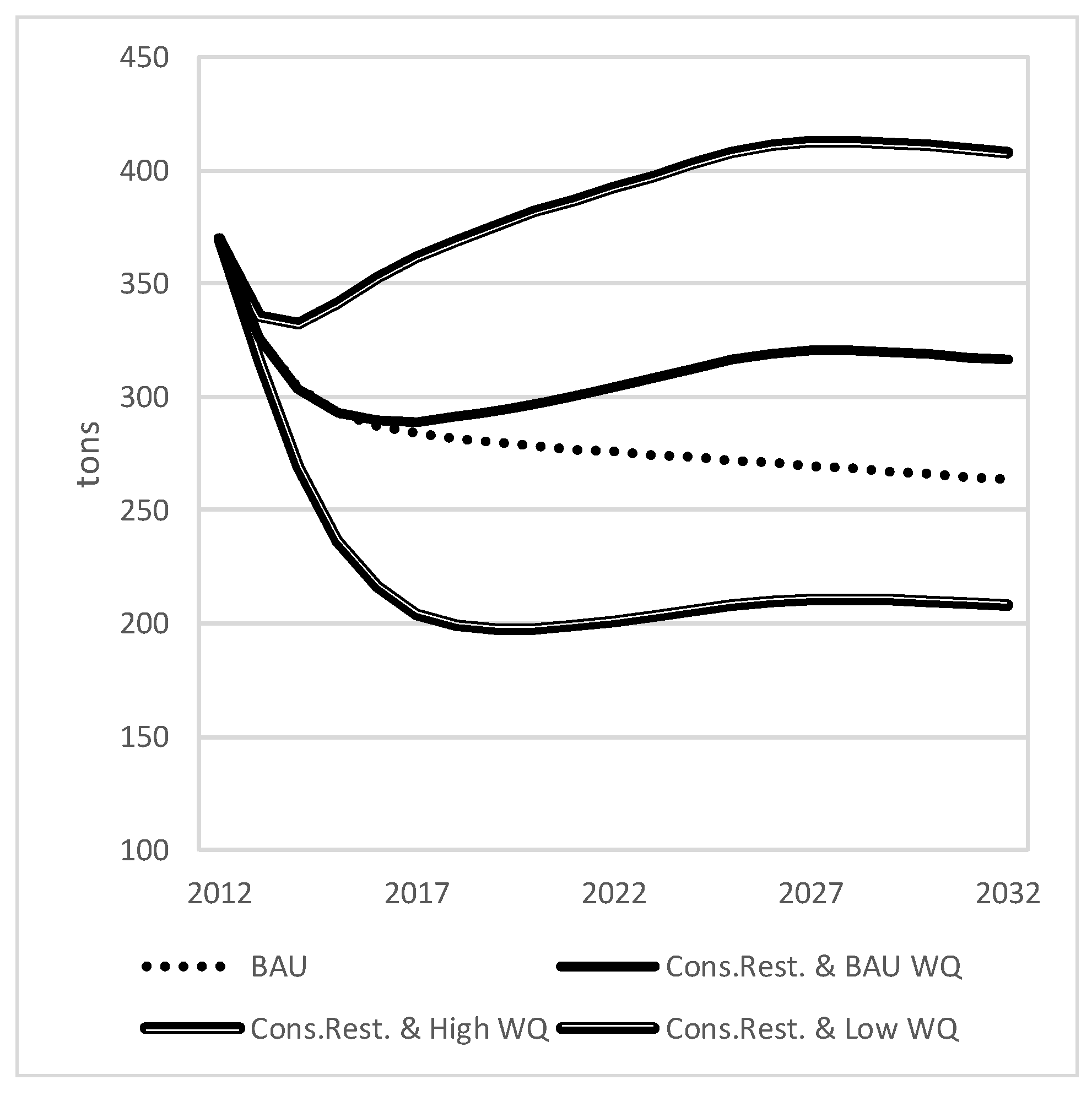
3.1. Policy Impact Assessments

Figure 6a–d show the impacts of restoration schedules with cost allocation rule 1 on the outcome indicators over time except for GOSs, which will be shown later, separately. Results with cost allocation rule 2 are not presented because they are very similar, although not identical to those detailed here. In other words, the choice of the cost allocation rule does not have significant impact on these four outcome indicators. Economic outcome indicators (GDP and disposable income) are lower with restoration than at the BAU level—because of restoration costs—whereas the opposite holds for ecological outcome indicators (total surface of nursery areas and soles caught). Restoration schedule also plays a role, as increasing restoration rate over time (the “Increasing” scenario) is preferred for economic outcomes (Figure 6a,b), whereas faster restoration early in time (the “Decreasing” scenario) is preferred for ecological outcomes (Figure 6c,d).

Figure 7 shows the impacts of restoration schedules on selected GOSs from 37 sectors to highlight the sectoral differences. Figure 7a–c suggest that, irrespective of the cost allocation rule, the total GOS earned by all companies in the region is lower with restoration than without restoration (BAU).

The cost allocation rule matters for the transport sector (Figure 7d–f) because it reduces the GOS, as harbors (which are included in the transport sector category) are bearing 100% and 49.75% of the cost in rules 1 and 2, respectively. Rule 2 (“Sharing”) reduces the impact, as other sectors acting later in the supply chain share the restoration cost. For the other sectors and total GOS, the choice of the cost allocation rule does not make any visible difference so that lines for rules 1 and 2 overlap.

The construction sector benefits from the restoration because it implements it and thereby increases its GOS. However, negative impacts outweigh positive ones (Figure 7g–i). Indeed, during the restoration period, economic growth slows in the region, thereby reducing household consumption and inducing a slowdown for the construction sector through indirect linkages with the other sectors of the regional economy.

Figure 7j–l show a reduction in GOS for the textile sector across all three scenarios, in opposition with the aggregate figures (Figure 7a–c). This reflects the downward technical coefficients of the dynamized IO (Figure 2). This captures the past and current trend in the textile sector. French production has increasingly been substituted by imports from developing and emergent countries in which labor costs are much lower. Between 1994 and 2015, the output of the French textile industry decreased by 60% (own calculation in IO data from INSEE [55]).

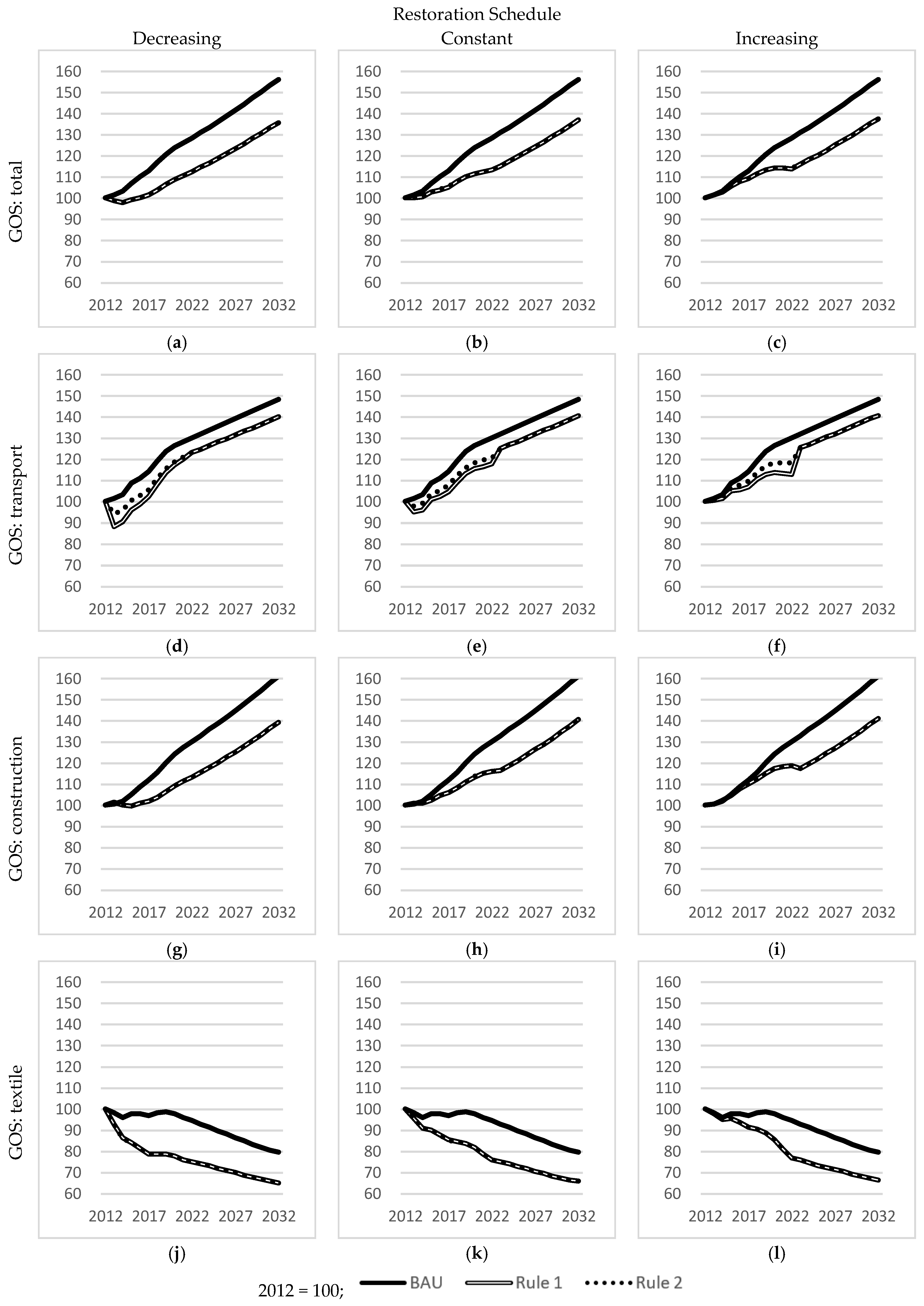
3.2. Policy Sensitivity Analysis

We conducted a policy sensitivity analysis to explore how water quality level (WQ) influences policy recommendations. We only present the impact on soles caught because other outcome indicators were barely affected (see Supplementary Information for summary statistics) and there is no impact on nursery areas because their dynamics are exogenously determined by the restoration scenarios.

There are two important results. First, Figure 8 shows the impacts of water quality on soles caught when restoration is implemented. The results for High WQ and Low WQ correspond respectively to the largest and smallest values of soles caught computed by the sensitivity analysis. Since water quality improvement positively contributes to the abundance of juvenile soles (Equation (10) and Figure 3), it is reasonable to assume that better WQ leads to larger quantities of soles caught (Cons.Rest. and High WQ) than BAU WQ (Cons.Rest. and BAU WQ) throughout the simulation period. In total, the cumulated amount of soles caught is 8084 tons for high water quality, which is 23.9% higher than the BAU level (6527 tons).

While Figure 8 showed the combined impact of restoration and various WQ levels on soles caught, Figure 9 now compares the impact of restoration on soles caught with three scenarios (“Constant”, “Decreasing”, and “Increasing”: Figure 4) and that of water quality improvement without restoration. The purpose is to explore how much water quality improvement contributes to the quantity of soles caught. As Figure 9 shows, if water quality greatly improves, without restoration, soles caught could be higher than with any restoration scenarios (e.g., High WQ). In cumulative values, although better water quality (High WQ) can improve soles caught by 23.3% (7332 tons) compared to BAU levels (5945 tons), the “Decreasing” restoration scenario (Dec.Rest.) improves the catch by 11.6%. There is, of course, a possibility that low water quality (e.g., Low WQ) leads to less catch (27.5% lower).

The best policy recommendation in terms of soles caught would therefore seem to hope for the best WQ level possible. However, as this seems unrealistic or at least difficult to achieve, an interesting policy option candidate (whose end result is close to high WQ level) would be restoration at a decreasing rate; that is, undertake more effort today and less in the future to arrive at the predetermined restoration target.

4. Discussion

4.1. Model Development and Analysis

We developed a fully dynamic IO/SD ecological-economic model by extending [16] with dynamization of the technical coefficients in the IO component so the model captures dynamic relationships within and between the ecological and economic systems.

Our fully dynamic model is an answer to criticisms about constant technical coefficients, showing that changes in technical coefficients differ by sector and that their magnitude [37] and directions of change (positive or negative) seem to be reasonable. The dynamization of IO shows a sharp contrast within various sectors when restoration policies are implemented (Figure 7).

We used econometrics, more precisely GLS, to evolve from a static to dynamic IO (see Equation (8)). Other techniques could have been investigated for capturing changes that are not an extension of the past, including using experts’ opinions on future technological changes [56] and the RAS method [57], for example.

We then analyzed the IO/SD model by developing various scenarios that explore the complex behavior of the ecological-economic system as applied in the Millennium Ecosystem Assessment [44]. By taking advantage of the SD software, we combined policy impact and policy sensitivity analyses to develop various scenarios. Whether assessment indicators are barely or significantly impacted by restoration and water quality improvement, all cases reflect dynamic interactions between and within the ecological-economic model. Hence, both findings seem relevant.

Varying restoration schedules revealed trade-offs between economic impacts and ecological benefits. Also, the sectoral analyses undertaken in this paper showed that the overall negative impacts of the economic slowdown due to restoration costs outweigh the benefits for the regional economy, mostly materialized by advantages for the construction sector.

The policy sensitivity analysis using water quality improvement identified the potential importance of examining exogenous factors outside the system boundary. Water quality is exogenously given (it is beyond the regional authorities’ control) and our analyses show that its improvement could increase soles caught by a greater amount than any restoration policy. Hence, water quality should be a priority for research and public policy aimed at restoring fish nursery habitats. Obviously, improving water quality will result in economic costs for the region. Also, because the Seine River’s water quality depends on neighboring river bodies [43], coordination between regions and countries seems essential and economic costs may be shared. To quantify the economic and ecological consequences of water quality improvement resulting from changes in industrial processes, agricultural practices and urban waste water treatment plants, a full hydrological and biogeochemical model of the Seine-Normandie water basin should be developed for many contaminants (HAPs, Nitrates, Phosphates, organic matter, heavy metals, pesticides, residual medical drugs, plastic chemicals such as Bisphenol-A, etc.). However, this is a real scientific challenge given the huge surface area of the Seine-Normandie (95,000 km²) extending from the Seine estuary, downstream, to Paris city, upstream, and including almost 200,000 industries and 18 million inhabitants. However, developing such a model is beyond current scientific capacities and should be developed in future research [58].

4.2. Future Research Topics

Despite the potential importance of IO/SD models [10,11,12], the development of such models has been rare. Our study paves the way for a new generation of ecological-economic models based on IO/SD, leaving room for future research on modeling and environmental policy analysis.

First, research on sustainability indicators and ecological-economic modeling should be undertaken together [10,59]. Our model captured the correlations and trade-offs between sustainability indicators, but research on sustainability indicators [60] often does not reflect the relationships between them, ignoring their interdependencies. In turn, indicator selection can guide ecological-economic modeling [61], as a model should be built for a specific purpose [29], such as capturing the dynamics and relationships between sustainability indicators. Our model was not systematically guided by indicator selection.

Second, improving the degree of system closure in economic components by adding an econometric analysis could further improve modeling. Indeed, keeping final demands exogenous, such as in most IO models, may undervalue socio-economic changes [36], but regional IO-econometric models could improve inter-industry impact studies [13,36,37,38]. In our model, two final demand categories are endogenous: household consumption (computed as a function of incomes) and investments (computed as a function of profit). However, both are partly based on an exogenous parameter: household consumption includes exogenous income elasticities ($e_i$) and investments are based on a fixed capital formation coefficient (${\widehat{cap}}_i$) calculated in the IO table at the reference year. Future research should replace exogenous parameters with statistical regressions computed from time series data related to the studied area.

Finally, other sources of complexity can be added. For example, our model did not reflect resilience. We might want to add a threshold value of fish population below which the fish stock becomes extinct in a way to help improve sustainable management of the Eastern Channel as suggested in a recent ICES report [62].

References

1. Limburg, K.E.; O’Neill, R.V.; Costanza, R.; Farber, S. Complex systems and valuation. Ecol. Econ. 2002, 41, 409–420. [Google Scholar] [CrossRef]
2. Costanza, R.; Wainger, L.; Folke, C.; Mäler, K.G. Modeling complex ecological economic systems. Bioscience 1993, 43, 545–555. [Google Scholar] [CrossRef]
3. Costanza, R.; Ruth, M. Using dynamic modeling to scope environmental problems and build consensus. Environ. Manag. 1998, 22, 183–195. [Google Scholar] [CrossRef]
4. Arrow, K.; Dasgupta, P.; Mäler, K.G. Evaluating projects and assessing sustainable development in imperfect economies. Environ. Resour. Econ. 2003, 26, 647–685. [Google Scholar] [CrossRef]
5. Dasgupta, P.; Mäler, K.G. The economics of non-convex ecosystems: Introduction. Environ. Resour. Econ. 2003, 26, 499–525. [Google Scholar] [CrossRef]
6. Uehara, T. Ecological threshold and ecological economic threshold: Implications from an ecological economic model with adaptation. Ecol. Econ. 2013, 93, 374–384. [Google Scholar] [CrossRef]
7. Levin, S.; Xepapadeas, T.; Crépin, A.-S.; Norberg, J.; de Zeeuw, A.; Folke, C.; Hughes, T.; Arrow, K.; Barrett, S.; Daily, G.; et al. Social-ecological systems as complex adaptive systems: Modeling and policy implications. Environ. Dev. Econ. 2013, 18, 111–132. [Google Scholar] [CrossRef]
8. Folke, C.; Carpenter, S.; Elmqvist, T.; Gunderson, L.; Holling, C.S.; Walker, B. Resilience and sustainable development: Building adaptive capacity in a world of transformations. AMBIO A J. Hum. Environ. 2002, 31, 437–440. [Google Scholar] [CrossRef]
9. Schlüter, M.; Hinkel, J.; Bots, P.; Arlinghaus, R. Application of the SES framework for model-based analysis of the dynamics of social-ecological systems. Ecol. Soc. 2014, 19, 36. [Google Scholar] [CrossRef]
10. Costanza, R.; Daly, L.; Fioramonti, L.; Giovannini, E.; Kubiszewski, I.; Mortensen, L.F.; Pickett, K.E.; Ragnarsdottir, K.V.; De Vogli, R.; Wilkinson, R. Modelling and measuring sustainable wellbeing in connection with the UN Sustainable Development Goals. Ecol. Econ. 2016, 130, 350–355. [Google Scholar] [CrossRef]
11. Hardt, L.; O’Neill, D.W. Ecological macroeconomic models: Assessing current developments. Ecol. Econ. 2017, 134, 198–211. [Google Scholar] [CrossRef]
12. Motesharrei, S.; Rivas, J.; Kalnay, E.; Asrar, G.R.; Busalacchi, A.J.; Cahalan, R.F.; Cane, M.A.; Colwell, R.R.; Feng, K.; Franklin, R.S.; et al. Modeling sustainability: Population, inequality, consumption, and bidirectional coupling of the Earth and Human Systems. Natl. Sci. Rev. 2016, 3, 470–494. [Google Scholar] [CrossRef]
13. Kim, K.; Kratena, K.; Hewings, G.J.D. The extended econometric input-output model with heterogeneous household demand system. Econ. Syst. Res. 2015, 27, 257–285. [Google Scholar] [CrossRef]
14. Miller, R.E.; Blair, P.D. Input-Output Analysis; Cambridge University Press: Cambridge, UK, 2009. [Google Scholar]
15. Berg, M.; Hartley, B.; Richters, O. A stock-flow consistent input-output model with applications to energy price shocks, interest rates, and heat emissions. New J. Phys. 2015, 17. [Google Scholar] [CrossRef]
16. Cordier, M.; Uehara, T.; Weih, J.; Hamaide, B. An input-output economic model integrated within a system dynamics ecological model: Feedback loop methodology applied to fish nursery restoration. Ecol. Econ. 2017, 140, 46–57. [Google Scholar] [CrossRef]
17. Jackson, T.; Drake, B.; Victor, P.; Kratena, K.; Sommer, M. Foundations for an Ecological Macroeconomics: Literature Review and Model Development; WWWforEurope Working Paper, No. 65; WWWforEurope: Vienna, Austria, 2014. [Google Scholar]
18. Gilbert, N. Agent-Based Models; Sage Publications: Thousand Oaks, CA, USA, 2008. [Google Scholar]
19. Boumans, R.; Costanza, R.; Farley, J.; Wilson, M.A.; Portela, R.; Rotmans, J.; Villa, F.; Grasso, M. Modeling the dynamics of the integrated earth system and the value of global ecosystem services using the GUMBO model. Ecol. Econ. 2002, 41, 529–560. [Google Scholar] [CrossRef]
20. Motesharrei, S.; Rivas, J.; Kalnay, E. Human and nature dynamics (HANDY): Modeling inequality and use of resources in the collapse or sustainability of societies. Ecol. Econ. 2014, 101, 90–102. [Google Scholar] [CrossRef]
21. Uehara, T.; Nagase, Y.; Wakeland, W. Integrating economics and system dynamics approaches for modelling an ecological-economic system. Syst. Res. Behav. Sci. 2015, 33, 515–531. [Google Scholar] [CrossRef]
22. Swinerd, C.; McNaught, K.R. Design classes for hybrid simulations involving agent-based and system dynamics models. Simul. Model. Pract. Theory 2012, 25, 118–133. [Google Scholar] [CrossRef] [Green Version]
23. Wallentin, G.; Neuwirth, C. Dynamic hybrid modelling: Switching between AB and SD designs of a predator-prey model. Ecol. Model. 2017, 345, 165–175. [Google Scholar] [CrossRef]
24. Cuvilliez, A.; Deloffre, J.; Lafite, R.; Bessineton, C. Morphological responses of an estuarine intertidal mudflat to constructions since 1978 to 2005: The Seine estuary (France). Geomorphology 2009, 104, 165–174. [Google Scholar] [CrossRef]
25. Rochette, S.; Rivot, E.; Morin, J.; Mackinson, S.; Riou, P.; Le Pape, O. Effect of nursery habitat degradation on flatfish population: Application to Solea solea in the Eastern Channel (Western Europe). J. Sea Res. 2010, 64, 34–44. [Google Scholar] [CrossRef]
26. HAROPA Ports de Paris Seine Normandie. Rapport D’activité 2013; HAROPA Ports de Paris Seine Normandie: Paris, France, 2013. [Google Scholar]
27. Ducrotoy, J.P.; Dauvin, J.C. Estuarine conservation and restoration: The Somme and the Seine case studies (English Channel, France). Mar. Pollut. Bull. 2008, 57, 208–218. [Google Scholar] [CrossRef] [PubMed]
28. Tecchio, S.; Chaalali, A.; Raoux, A.; Tous Rius, A.; Lequesne, J.; Girardin, V.; Lassalle, G.; Cachera, M.; Riou, P.; Lobry, J.; et al. Evaluating ecosystem-level anthropogenic impacts in a stressed transitional environment: The case of the Seine estuary. Ecol. Indic. 2015, 61, 833–845. [Google Scholar] [CrossRef]
29. Sterman, J.D. Business Dynamics: Systems Thinking and Modeling for a Complex World; Irwin/McGraw-Hill Boston: Boston, MA, USA, 2000. [Google Scholar]
30. European Commission. ESA Supply, Use and Input-Output Tables. 2014. Available online: http://ec.europa.eu/eurostat/web/esa-supply-use-input-tables (accessed on 27 May 2018).
31. Jackson, R.W. Regionalizing national commodity-by-industry accounts. Econ. Syst. Res. 1998, 10, 223–238. [Google Scholar] [CrossRef]
32. Lahr, M.L. Reconciling domestication techniques, the notion of Re-exports and some comments on regional accounting. Econ. Syst. Res. 2001, 13, 165–179. [Google Scholar] [CrossRef]
33. McDonald, G. Integrating Economics and Ecology: A Systems Approach to Sustainability in the Auckland Region. PhD Thesis, Massey University, Palmerston North, New Zealand, 2005. [Google Scholar]
34. Gohin, A. The specification of price and income elasticities in computable general equilibrium models: An application of latent separability. Econ. Model. 2005, 22, 905–925. [Google Scholar] [CrossRef]
35. Klein, L.R.; Welfe, A.; Welfe, W. Principles of Macroeconometric Modeling; North-Holland Publishing Co.: Amsterdam, The Netherlands, 1999. [Google Scholar]
36. Conway, R.S. The Washington projection and simulation model: A regional interindustry econometric model. Int. Reg. Sci. Rev. 1990, 13, 141–165. [Google Scholar] [CrossRef]
37. Israilevich, P.R.; Hewings, G.J.D.; Schindler, G.R.; Mahidhara, R. The choice of an input-output table embedded in regional econometric input-output models. Pap. Reg. Sci. 1996, 75, 103–119. [Google Scholar] [CrossRef]
38. Israilevich, P.R.; Hewings, G.J.D.; Sonis, M.; Schindler, G.R. Forecasting structural change with a regional econometric input-output model. J. Reg. Sci. 1997, 37, 565–590. [Google Scholar] [CrossRef]
39. FCBA. Balance Commerciale de la Filière Forêt-Bois en 2016. 2017. Available online: http://www.fcba.fr/actualite/balance-commerciale-de-la-filiere-foret-bois-en-2016 (accessed on 20 February 2018).
40. Copacel. Les Statistiques de L’industrie Papetière Française; Rapport Développement Durable; Copacel: Paris, France, 2012. [Google Scholar]
41. INSEE. Tableau des Entrées-Sorties, Niveau 38 (En Millions D’euros). 2017. Available online: https://www.insee.fr/fr/statistiques/2832720?sommaire=2832834&q=tableaux+entr%C3%A9e-sortie#titre-bloc-114 (accessed on 20 February 2018).
42. Pankhurst, N.W.; Munday, P.L. Effects of climate change on fish reproduction and early life history stages. Mar. Freshw. Res. 2011, 62, 1015–1026. [Google Scholar] [CrossRef]
43. Romero, E.; Le Gendre, R.; Garnier, J.; Billen, G.; Fisson, C.; Silvestre, M.; Riou, P. Long-term water quality in the lower Seine: Lessons learned over 4 decades of monitoring. Environ. Sci. Policy 2016, 58, 141–154. [Google Scholar] [CrossRef]
44. Alcamo, J.; Vuuren, D.; Ringler, C.; Alder, J.; Bennett, E.M.; Lodge, D.; Masui, T.; Morita, T.; Rosegrant, M.; Sala, O. Methodology for developing the MA scenarios. Ecosyst. Hum. Well-Being Scenar. 2005, 2, 145–172. [Google Scholar]
45. OECD. Guidance on Sustainability Impact Assessment; OECD Publishing: Paris, France, 2010. [Google Scholar]
46. European Commission. Impact Assessments. n.d. Available online: https://ec.europa.eu/info/law/law-making-process/planning-and-proposing-law/impact-assessments_en (accessed on 18 February 2018).
47. Cordier, M.; Poitelon, T.; Hecq, W. Developing a Shared Environmental Responsibility Principle for Distributing Cost of Restoring Marine Habitats Destroyed by Industrial Harbors (No. 18/008); CEB Working Paper; ULB—Universite Libre de Bruxelles: Bruxelles, Belgium, 2018. [Google Scholar]
48. OECD. Recommendation of the Council on Guiding Principles Concerning International Economic Aspects of Environmental Policies; OECD: Paris, France, 1972. [Google Scholar]
49. OECD. Recommendation of the Council on the Implementation of the Polluter-Pays Principle; OECD: Paris, France, 1974. [Google Scholar]
50. Gallego, B.; Lenzen, M. A consistent input-output formulation of shared producer and consumer responsibility. Econ. Syst. Res. 2005, 17, 365–391. [Google Scholar] [CrossRef]
51. Lenzen, M.; Murray, J.; Sack, F.; Wiedmann, T. Shared producer and consumer responsibility—Theory and practice. Ecol. Econ. 2007, 61, 27–42. [Google Scholar] [CrossRef]
52. Lenzen, M.; Murray, J. Conceptualising environmental responsibility. Ecol. Econ. 2010, 70, 261–270. [Google Scholar] [CrossRef]
53. Rosenberger, R.S.; Loomis, J.B. Benefit transfer. In A Primer on Nonmarket Valuation; Champ, P.A., Boyle, K.J., Brown, T.C., Eds.; Springer: Dordrecht, The Netherlands, 2017; pp. 445–482. [Google Scholar]
54. Van der Ploeg, S.; De Groot, R.S. The TEEB Valuation Database—A Searchable Database of 1310 Estimates of Monetary Values of Ecosystem Services; Foundation for Sustainable Development: Wageningen, The Netherlands, 2010. [Google Scholar]
55. INSEE. Tableaux Entrées Sorties Niveau 38. n.d. Available online: https://www.insee.fr/fr/statistiques/2383687?sommaire=2383694 (accessed on 20 February 2018).
56. Duchin, F.; Lange, G.-M. The Future of the Environment: Ecological Economics and Technological Change; Oxford University Press on Demand: Oxford, UK, 1994. [Google Scholar]
57. Rao, M.; Tommasino, M.C. Updating Technical Coefficients of an Input-Output Matrix with RAS-The trIOBAL Sofware. A VBA/GAMS Application to Italian Economy for Years 1995 and 2000; ENEA: Rome, Italy, 2014. [Google Scholar]
58. Briand, C.; Gateuille, D.; Gasperi, J.; Moreau-Guigon, E.; Alliot, F.; Chevreuil, M.; Blanchard, M.; Teil, M.-J.; Brignon, J.-M.; Labadie, P.; et al. Bilans et Flux de Polluants Organiques Dans le Bassin de la Seine; PIREN-Seine—Phase VII—Repport; PIREN-Seine: Paris, France, 2016. [Google Scholar]
59. Uehara, T.; Mineo, K. Regional sustainability assessment framework for integrated coastal zone management: Satoumi, ecosystem services approach, and inclusive wealth. Ecol. Indic. 2017, 73, 716–725. [Google Scholar] [CrossRef]
60. Singh, R.K.; Murty, H.R.; Gupta, S.K.; Dikshit, A.K. An overview of sustainability assessment methodologies. Ecol. Indic. 2012, 9, 281–299. [Google Scholar] [CrossRef]
61. Schlüter, M.; Baeza, A.; Dressler, G.; Frank, K.; Groeneveld, J.; Jager, W.; Janssen, M.A.; McAllister, R.R.J.; Müller, B.; Orach, K.; et al. A framework for mapping and comparing behavioural theories in models of social-ecological systems. Ecol. Econ. 2017, 131, 21–35. [Google Scholar] [CrossRef]
62. ICES. Report of the Working Group on Assessment of Demersal Stocks in the North Sea and Skagerrak, 26 April–5 May 2017, ICES HQ, ICES CM; ICES: Copenhagen, Denmark, 2017. [Google Scholar]
Figure 1. Interconnections between the economic sub-system and ecological system. The figure is adapted from [16] with primary model extensions underlined in red. Note: “+” and “−” indicate variable changes in the “same” and “opposite” direction, respectively.
Sustainability 10 01765 g001
Figure 2. Changes in technical coefficients for the 37 sectors (positive changes are in dark color, negative ones in lighter color, and white cells mean no change). See S1 for regression models used for creating the figure. See S2 for the full descriptions of sector names.
Sustainability 10 01765 g002
Figure 3. The IO/SD model of the ecological system and its economic sub-system (Stocks and flows are represented by boxes and double arrows respectively. Circles and diamonds denote auxiliary variables and constants).
Sustainability 10 01765 g003
Figure 4. Three representative restoration schedules. (a) Increasing; (b) Constant; (c) Decreasing.
Sustainability 10 01765 g004
Figure 5. Cost allocation rule under the “sharing” mechanism.
Sustainability 10 01765 g005
Figure 6. Impacts of restoration schedules with cost allocation rule 1. See Table S1 for the cumulative values of the impacts of restoration over the simulation period displayed in Figure 6.
Sustainability 10 01765 g006
Figure 7. Impact of restoration schedule and cost allocation rule on selected GOSs. See Table S2 for the cumulative values of the impacts displayed in Figure 7.
Sustainability 10 01765 g007
Figure 8. Soles caught. Cons.Rest. stands for restoration at constant rate. WQ stands for water quality. Cons.Rest. and High WQ and Cons.Rest. and Low WQ are computed by the sensitivity analysis with varying WQ index. Cost allocation rule 1 is applied. See Tables S3–S5 for more detailed results of the sensitivity analysis.
Sustainability 10 01765 g008
Figure 9. Soles caught to compare the contributions of restoration vs. water quality. High WQ and Low WQ are computed by the sensitivity analysis with varying WQ index. See Tables S6–S8 for more detailed results of the sensitivity analysis.
Sustainability 10 01765 g009