Analysis of the Land Use and Cover Changes in the Metropolitan Area of Tepic-Xalisco (1973–2015) through Landsat Images

 , ,
, ,
Abstract
:1. Introduction
2. Materials and Methods
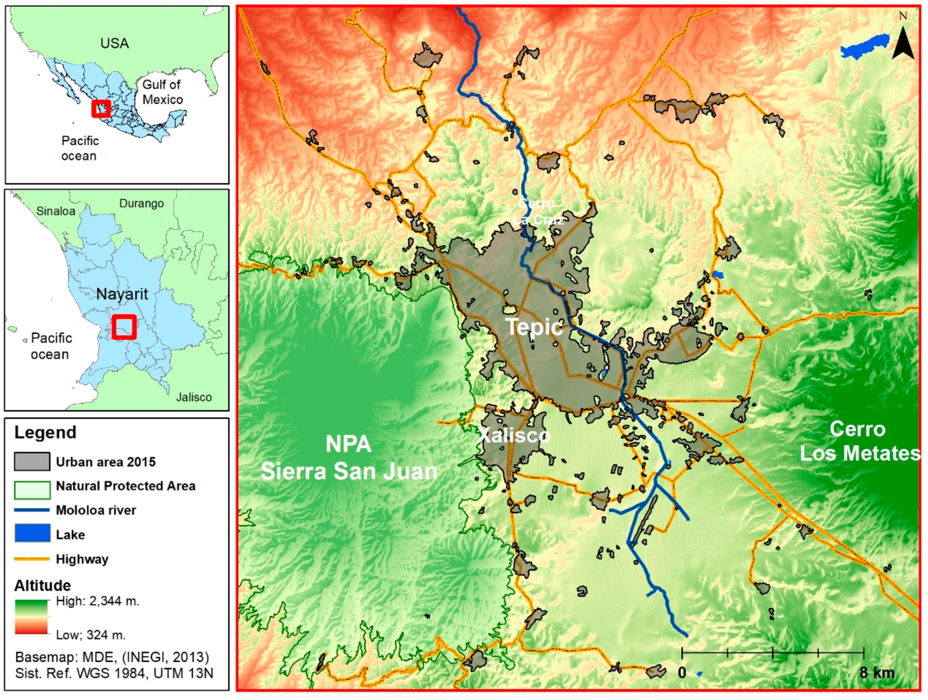
2.1. Study Area
2.2. Data
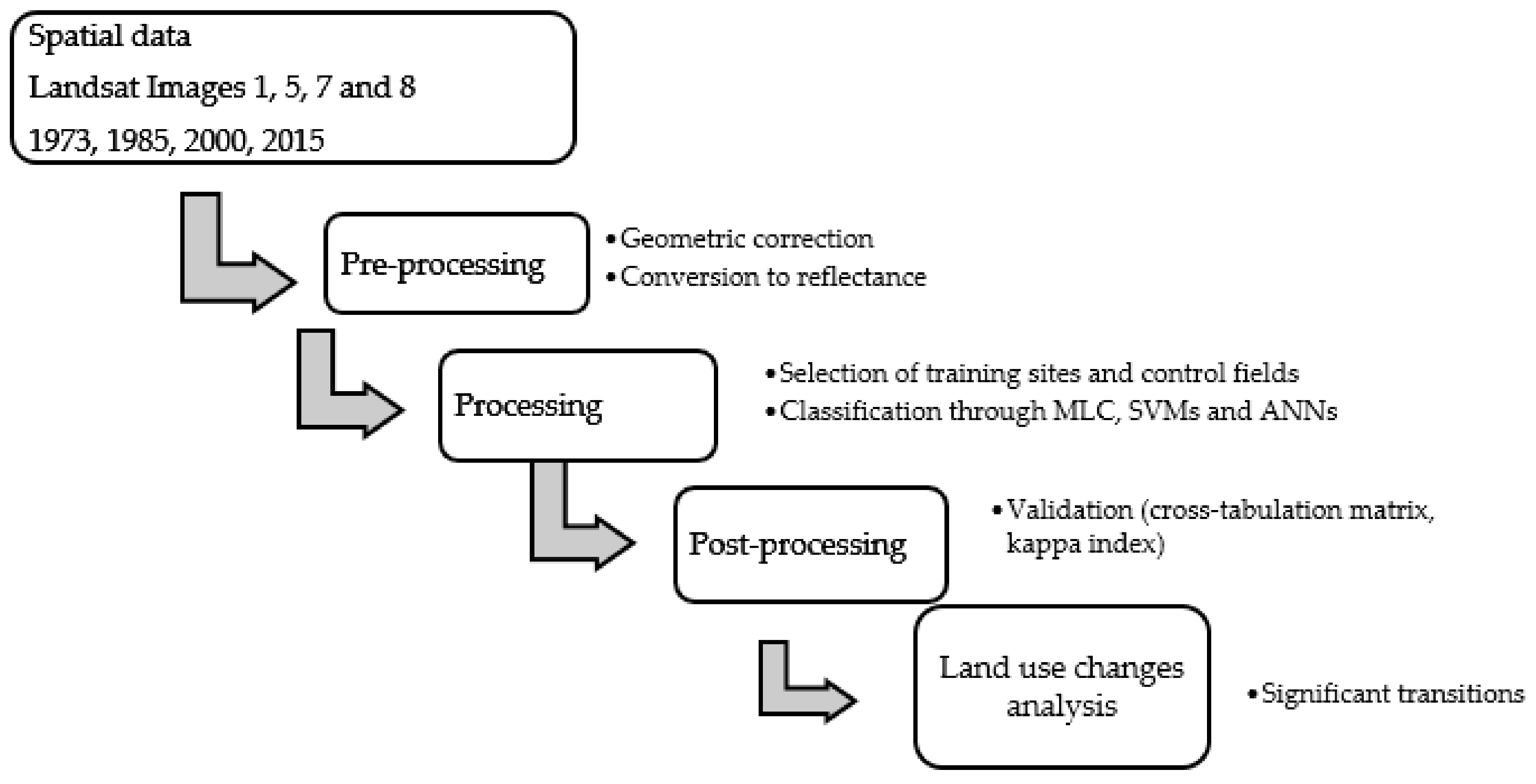
2.3. Methodology
3. Satellite Images Classification
3.1. Pre-Processing
3.2. Processing
3.3. Post-Processing
3.4. Analysis of Land Use and Cover Changes
4. Results and Discussion
4.1. Satellite Images Classification
4.2. Classification Validation
4.3. Analysis of Land Use Changes
5. Conclusions
Author Contributions
Acknowledgments
Conflicts of Interest
References
- Aguayo, M.; Pauchard, A.; Azócar, G.; Parra, O. Cambio del uso del suelo en el centro sur de Chile a fines del siglo XX. Entendiendo la dinámica espacial y temporal del paisaje. Rev. Chil. Hist. Nat. 2009, 82, 361–374. [Google Scholar] [CrossRef]
- Mas, J.F.; Velázquez, A.; Reyes, D.G.J.; Mayorga, S.R.; Alcántara, C.; Bocco, G.; Castro, R.; Fernandez, T.; Perez, V.A. Assessing land use/cover changes: A nationwide multidate spatial database for Mexico. Int. J. Appl. Earth Obs. Geoinf. 2004, 5, 249–261. [Google Scholar] [CrossRef]
- Mendoza, E.; Dirzo, R. Deforestation in Lacandonia (southeast Mexico): Evidence for the declaration of the northernmost tropical hot-spot. Biodivers. Conserv. 1999, 8, 1621–1641. [Google Scholar] [CrossRef]
- Lambin, E.F.; Turner, B.L.; Helmut, J.; Geist, S.B.; Agbola, S.B.; Arild, A.; Bruce, J.W.; Coomes, O.T.; Dirzo, R.; Fischer, G.; et al. The causes of land-use and land-cover change: Moving beyond the myths. Glob. Environ. Chang. 2001, 11, 261–269. [Google Scholar] [CrossRef]
- Turner, B.L.; Lambin, E.F.; Reenberg, A. The emergence of land change science for global environmental change and sustainability. Proc. Natl. Acad. Sci. USA 2007, 104, 20666–20671. [Google Scholar] [CrossRef] [PubMed] [Green Version]
- Lambin, E.F.; Geist, H.J. (Eds.) Land-Use and Land-Cover Change: Local Processes and Global Impacts; Springer: Berlin, Germany, 2008. [Google Scholar]
- FAO. Evaluación de los Recursos Forestales Mundiales: Informe Nacional México; FAO: Roma, Italy, 2010; Available online: http://www.fao.org/docrep/013/al567S/al567S.pdf (accessed on 31 May 2018).
- Bocco, G.; Mendoza, M.; Masera, O.R. La Dinámica del Cambio del Uso del Suelo en Michoacán: Una Propuesta Metodológica para el Estudio de los Procesos de Deforestación. Investig. Geogr. 2001, 44, 18–36. Available online: http://www.redalyc.org/articulo.oa?id=56904403 (accessed on 31 May 2018). [CrossRef]
- Velázquez, A.; Durán, E.; Ramírez, I.; Mas, J.F.; Bocco, G.; Ramírez, G.; Palacio, J.L. Land use-cover change processes in highly biodiverse areas: The case of Oaxaca, México. Glob. Environ. Chang. 2003, 13, 175–184. [Google Scholar] [CrossRef]
- Velázquez, A.; Mas, J.F.; Díaz, G.J.R.; Mayorga, S.R.; Alcántara, P.C.; Castro, R.; Fernández, T.; Bocco, G.; Ezcurra, E.; Palacio, J.L. Patrones y tasas de cambio de uso del suelo en México. Gaceta Ecol. 2002, 62, 21–37. [Google Scholar]
- Millennium Ecosystem Assessment. Ecosystems. 2003. Available online: https://www.millenniumassessment.org/en/index.html (accessed on 31 May 2018).
- SEMARNAT. Informe de la Situación del Medio Ambiente en México; SEMARNAT: México City, México, 2012. Available online: http://apps1.semarnat.gob.mx/dgeia/informe_12/pdf/Informe_2012.pdf (accessed on 31 May 2018).
- Challenger, A.; Soberón, J. Los Ecosistemas Terrestres, en Capital Natural de México, vol. I: Conocimiento Actual de la Biodiversidad; CONABIO: México City, México, 2008; pp. 87–108. Available online: http://www.biodiversidad.gob.mx/pais/pdf/CapNatMex/Vol%20I/I03_Losecosistemast.pdf (accessed on 31 May 2018).
- Galicia, L.; García, R.A.; Gómez-Mendoza, L.; Ramírez, M.I. Cambio de uso del suelo y degradación ambiental. Ciencia 2007, 584, 50–59. [Google Scholar]
- Mas, J.F.; Velázquez, A.; Couturier, S. La evaluación de los cambios de cobertura/uso del suelo en la República Mexicana. Investigación Ambiental Ciencia y Política Pública 2009, 1, 23–39. [Google Scholar]
- Chuvieco, E. Teledetección Ambiental: La Observación de la Tierra Desde el Espacio (Editorial Ariel). 2008. Available online: https://drive.google.com/file/d/0B0KUmy_fthbuX09sUE9RejJJX1U/view (accessed on 31 May 2018).
- Civco, D.L.; Hurd, J.D.; Wilson, E.H.; Song, M.; Zhang, Z. A Comparison of Land Use and Land Cover Change Detection Methods. In Proceedings of the ASPRS-ACSM Annual Conference, Washington, DC, USA, 22–26 April 2002; Available online: https://www.researchgate.net/profile/Daniel_Civco/publication/228543190_A_comparison_of_land_use_and_land_cover_change_detection_methods/links/5570b54608aedcd33b292ec1.pdf (accessed on 31 May 2018).
- Monjardín, A.S.A.; Pacheco, A.C.E.; Plata, R.W.; Corrales, B.G. La deforestación y sus factores causales en el estado de Sinaloa, México. Madera y Bosques 2017, 231, 7–22. [Google Scholar] [CrossRef]
- Pontius, R.G.; Shusas, E.; McEachern, M. Detecting important categorical land changes while accounting for persistence. Agric. Ecosyst. Environ. 2004, 101, 251–268. [Google Scholar] [CrossRef]
- Chavez, P.S. Image-based atmospheric corrections. Revisited and improved. Photo-Gramm. Eng. Remote Sens. 1996, 62, 1025–1036. [Google Scholar]
- Bolstad, P.; Lillesand, T.M. Rapid maximum likelihood classification. Photogramm. Eng. Remote Sens. 1991, 571, 67–74. [Google Scholar]
- Hassan, Z.; Shabbir, R.; Ahmad, S.S.; Malik, A.H.; Aziz, N.; Butt, A.; Erum, S. Dynamics of land use and land cover change (LULCC) using geospatial techniques: A case study of Islamabad Pakistan. SpringerPlus 2016, 5, 1–11. [Google Scholar] [CrossRef] [PubMed]
- Tahir, M.; Iman, E.; Hussain, T. Evaluation of land use/land cover changes in Mekelle City. Ethiopia using Remote Sensing and GIS. Comput. Ecol. Softw. 2013, 3, 9–16. [Google Scholar]
- García Mora, T.J.; Mas, J.F. Comparación de metodologías para el mapeo de la cobertura y uso del suelo en el sureste de México. Investig. Geogr. 2008, 67, 7–19. [Google Scholar] [CrossRef]
- López, V.V.H.; Plata, R.W. Análisis de los cambios de cobertura de suelo derivados de la expansión urbana de la Zona Metropolitana de la Ciudad de México, 1990–2000. Investig. Geogr. 2009, 68, 85–101. [Google Scholar] [CrossRef]
- Vapnik, V.N. The Nature of Statistical Learning Theory; Springer: New York, NY, USA, 1995. [Google Scholar]
- Mountrakis, G.; Im, J.; Ogole, C. Support vector machines in remote sensing: A review. ISPRS J. Photogramm. Remote Sens. 2011, 66, 247–259. [Google Scholar] [CrossRef]
- Lu, D.; Weng, Q.; Moran, E.; Li, G.; Hetrick, S. Remote Sensing Image Classification; CRC Press; Taylor and Francis: Boca Raton, FL, USA, 2011; pp. 219–240. [Google Scholar]
- Xie, L.; Li, G.; Xiao, M.; Peng, L.; Chen, Q. Hyperspectral image classification using discrete space model and support vector machines. IEEE Geosci. Remote Sens. Lett. 2017, 14, 374–378. [Google Scholar] [CrossRef]
- Richards, J.A. Remote Sensing Digital Image Analysis; Springer: Berlin, Germany, 1999; p. 240. [Google Scholar]
- Atkinson, P.M.; Tatnall, A.R.L. Introduction Neural Networks in Remote Sensing. Int. J. Remote Sens. 1997, 184, 699–709. [Google Scholar] [CrossRef]
- Kavzoglu, T.; Mather, P.M. The use of backpropagating artificial neural networks in land cover classification. Int. J. Remote Sens. 2003, 24, 4907–4938. [Google Scholar] [CrossRef]
- Verbeke, L.P.C.; Vabcoillie, F.M.B.; Dewulf, R.R. Reusing back-propagating artificial neural network for land cover classification in tropical savannahs. Int. J. Remote Sens. 2004, 25, 2747–2771. [Google Scholar] [CrossRef]
- Antillón, V.M.Y.; Corral, G.G.M.; Alatorre, C.L.C. Análisis de los Cambios de Cobertura y uso de Suelo en los Márgenes de la Laguna de Bustillos, Chihuahua: Efectos de la Expansión Agrícola. Memorias de Resúmenes en Extenso SELPER-XXI-México-UACJ-2015. 2015. Available online: http://selper.org.mx/images/Memorias2015/assets/m005.pdf (accessed on 31 May 2018).
- Pal, M.; Mather, P.M. Support vector machines for classification in remote sensing. Int. J. Remote Sens. 2005, 26, 1007–1011. [Google Scholar] [CrossRef]
- Otukei, J.R.; Blaschke, T. Land cover change assessment using decision trees, support vector machines and maximum likehood classification algorithms. Int. J. Appl. Earth Obs. Geoinf. 2010, 12, S27–S31. [Google Scholar] [CrossRef]
- Mondal, A.; Kundu, S.; Chandniha, S.K.; Shukla, R.; Mishra, P.K. Comparison of support vector machine and maximum likelihood classification technique using satellite imagery. Int. J. Remote Sens. GIS 2012, 1, 116–123. [Google Scholar]
- Wu, W.; Li, A.D.; He, X.H.; Ma, R.; Liu, H.B.; Lv, J.K. A comparison of support vector machines, artificial neural network and classification tree for identifying soil texture classes in southwest China. Comput. Electron. Agric. 2018, 144, 86–93. [Google Scholar] [CrossRef]
- Camacho, S.J.M.; Pérez, J.; Isabel, J.; Pineda, J.N.B.; Cadena, V.E.G.; Bravo, P.L.C.; Sánchez, L.M. Cambios de cobertura/uso del suelo en una porción de la Zona de Transición Mexicana de Montaña. Madera y Bosques 2015, 21, 93–112. [Google Scholar]
- Evangelista, O.V.; López, B.J.; Caballero, N.J.; Martínez, A.M.Á. Patrones espaciales de cambio de cobertura y uso del suelo en el área cafetalera de la sierra norte de Puebla. Investig. Geogr. 2010, 72, 23–38. [Google Scholar] [CrossRef]
- Ramírez, R.I. Cambios en las Cubiertas del Suelo en la Sierra de Angangueo, Michoacán y Estado de México, 1971-1994-2000. Investig. Geogr. 2001, 45, 39–55. Available online: http://www.redalyc.org/pdf/569/56904504.pdf (accessed on 31 May 2018). [CrossRef]
- Guerrero, G.; Masera, O.; Mas, J.F. Land use/land cover change dynamics in the Mexican highlands: Current situation and long-term scenarios. In Modelling Environmental Dynamics; Springer: Berling, Germany, 2008; pp. 57–76. [Google Scholar]
- Pineda, J.N.B.; Bosque, S.J.; Gómez, D.M.; Plata, R.W. Análisis de cambio del uso del suelo en el Estado de México mediante sistemas de información geográfica y técnicas de regresión multivariantes: Una aproximación a los procesos de deforestación. Investig. Geogr. 2009, 69, 33–52. [Google Scholar]
- Cano, S.L.; Rodríguez, L.R.; Valdez, L.J.R.; Acevedo, S.O.A.; Beltrán, H.R.I. Detección del crecimiento urbano en el estado de Hidalgo mediante imágenes Landsat. Investig. Geogr. 2017, 92, 1–10. [Google Scholar] [CrossRef]
- Nájera, G.O.; Bojórquez, S.J.I.; Cifuentes, L.J.L.; Marceleño, F.S. Cambio de cobertura y uso del suelo en la cuenca del río Mololoa, Nayarit. Revista Bio Ciencias 2010, 1, 19–29. [Google Scholar] [CrossRef]


| Description | Image | Description | Image |
|---|---|---|---|
| Landsat 1 (1973) Multispectral Scanner System (MSS) Sensor LM10320451973043GDS03 Scene Spatial resolution 60 m Acquisition date 12 February 1973 Composition V-A-R |  | Landsat 5 (1985) Thematic Mapper (TM) Sensor LT50300451985139AAA03 Scene Spatial resolution 60 m Acquisition date 5 May 1985 Composition NIR-SWIR-R |  |
| Landsat 7 (2000) Enhanced Thematic Mapper (ETM) Sensor LE70300452000045EDC00 Scene Spatial resolution 30 m Acquisition date 14 February 2000 Composition NIR-SWIR-R |  | Landsat 8 (2015) Operational Land Imager (OLI) Sensor LO80300452015062LGN01 Scene Spatial resolution 30 m Acquisition date 3 April 2015 Composition NIR-SWIR-R |  |
| Class No. | Class | Description |
|---|---|---|
| 1 | Urban | Includes urban and industrial areas. |
| 2 | Agricultural | Periodic and temporary irrigation agriculture. |
| 3 | Water bodies | Water bodies, lakes and rivers. |
| 4 | Secondary vegetation | Includes arbustive (scrub and grassland) and arboreal vegetation of low or scarce density. |
| 5 | Forest | High density arboreal vegetation. |
| Year Evaluated | SVMs | MLC | ANNs | |||
|---|---|---|---|---|---|---|
| General Accuracy | Kappa Index | General Accuracy | Kappa Index | General Accuracy | Kappa Index | |
| 1973 | 98.7% | 0.98 | 97.7% | 0.96 | 97.7% | 0.96 |
| 1985 | 89.0% | 0.85 | 92.5% | 0.90 | 96.5% | 0.95 |
| 2000 | 89.3% | 0.85 | 82.1% | 0.76 | 92.7% | 0.90 |
| 2015 | 90.4% | 0.87 | 86.1% | 0.81 | 86.1% | 0.81 |
| Classified Image | Class | SVMs | MLC | ANNs | |||
|---|---|---|---|---|---|---|---|
| Producer’s Accuracy (%) | User’s Accuracy (%) | Producer’s Accuracy (%) | User’s Accuracy (%) | Producer’s Accuracy (%) | User’s Accuracy (%) | ||
| Landsat 1 MSS (1973) | Urban | 100 | 100 | 100 | 100 | 100 | 100 |
| Agricultural | 97 | 100 | 96 | 99 | 95 | 100 | |
| Water body | 100 | 100 | 100 | 100 | 100 | 100 | |
| Secondary vegetation | 100 | 95 | 100 | 93 | 100 | 98 | |
| Forest | 99 | 100 | 96 | 100 | 98 | 94 | |
| Landsat 5 TM (1985) | Urban | 100 | 100 | 100 | 100 | 83 | 199 |
| Agricultural | 100 | 100 | 100 | 100 | 100 | 98 | |
| Water body | 100 | 100 | 100 | 100 | 100 | 90 | |
| Secondary vegetation | 68 | 100 | 82 | 100 | 99 | 94 | |
| Forest | 100 | 74 | 100 | 83 | 93 | 100 | |
| Landsat 7 ETM (2000) | Urban | 100 | 100 | 100 | 56 | 100 | 39 |
| Agricultural | 100 | 100 | 93 | 100 | 89 | 98 | |
| Water body | 100 | 100 | 100 | 100 | 100 | 100 | |
| Secondary vegetation | 56 | 100 | 63 | 100 | 86 | 100 | |
| Forest | 100 | 67 | 100 | 71 | 100 | 89 | |
| Landsat 8 OLI (2015) | Urban | 100 | 100 | 100 | 100 | 94 | 89 |
| Agricultural | 100 | 80 | 100 | 94 | 95 | 84 | |
| Water body | 100 | 100 | 100 | 100 | 100 | 95 | |
| Secondary vegetation | 72 | 100 | 44 | 100 | 71 | 69 | |
| Forest | 100 | 96 | 100 | 76 | 83 | 93 | |
| Mean | 95 | 96 | 94 | 94 | 94 | 96 | |
| Classification Method | Class | Description | 1973 | 1985 | 2000 | 2015 | Annual Rate (km2) | ||||
|---|---|---|---|---|---|---|---|---|---|---|---|
| Area (km2) | Area (%) | Area (km2) | Area (%) | Area (km2) | Area (%) | Area (km2) | Area (%) | ||||
| SVMs | 1 | Urban | 6.8 | 1 | 19.2 | 2 | 40.0 | 4 | 68.8 | 8 | 1.48 |
| 2 | Agricultural | 151.1 | 17 | 215.1 | 24 | 342.8 | 38 | 211.3 | 23 | 1.43 | |
| 3 | Water body | 1.1 | 0 | 1.4 | 0 | 1.5 | 0 | 1.4 | 0 | 0.01 | |
| 4 | Secondary vegetation | 322.7 | 36 | 383.7 | 43 | 243.7 | 27 | 442.8 | 49 | 2.86 | |
| 5 | Forest | 418.3 | 46 | 280.6 | 31 | 272.1 | 30 | 175.7 | 20 | 5.78 * | |
| MLC | 1 | Urban | 6.8 | 1 | 19.2 | 2 | 39.9 | 4 | 68.6 | 8 | 1.47 |
| 2 | Agricultural | 179.5 | 20 | 258.1 | 29 | 234.7 | 26 | 218.5 | 24 | 0.93 | |
| 3 | Water body | 1.2 | 0 | 1.7 | 0 | 1.4 | 0 | 1.5 | 0 | 0.01 | |
| 4 | Secondary vegetation | 396.0 | 44 | 319.6 | 36 | 372.7 | 41 | 401.7 | 45 | 0.13 | |
| 5 | Forest | 316.4 | 35 | 301.3 | 33 | 251.3 | 28 | 209.7 | 23 | 2.54 * | |
| ANNs | 1 | Urban | 6.8 | 1 | 19.2 | 2 | 39.9 | 4 | 68.8 | 8 | 1.48 |
| 2 | Agricultural | 140.1 | 16 | 221.3 | 25 | 314.2 | 35 | 331.1 | 37 | 4.55 | |
| 3 | Water body | 1.1 | 0 | 2.6 | 0 | 2.1 | 0 | 1.8 | 0 | 0.02 | |
| 4 | Secondary vegetation | 281.2 | 31 | 413.4 | 46 | 283.6 | 32 | 284.4 | 32 | 0.08 | |
| 5 | Forest | 470.8 | 52 | 243.6 | 27 | 260.2 | 29 | 213.9 | 24 | 6.12 * | |
| Period | Class | Area (km2) | |||||||
|---|---|---|---|---|---|---|---|---|---|
| Total (t1) | Total (t2) | Steady (E) | Gains (G) | Losses (L) | Interchanges (I) | Net Change (NT) | Total Change (CT) | ||
| 1973–1985 | Urban | 6.8 | 19.2 | 6.8 | 12.4 | 0.0 | 0.0 | 12.4 | 12.4 |
| Agricultural | 151.1 | 215.1 | 86.6 | 128.5 | 64.5 | 129.0 | 64.0 | 193.0 | |
| Water body | 1.1 | 1.4 | 1.0 | 0.4 | 0.0 | 0.1 | 0.3 | 0.4 | |
| Secondary vegetation | 322.7 | 383.7 | 229.0 | 154.7 | 93.7 | 187.4 | 61.0 | 248.4 | |
| Forest | 418.3 | 280.6 | 263.0 | 17.6 | 155.3 | 35.2 | 137.7 | 172.9 | |
| 1985–2000 | Urban | 19.2 | 40.0 | 19.2 | 20.8 | 0.0 | 0.0 | 20.8 | 20.8 |
| Agriculture | 215.1 | 342.8 | 171.3 | 171.5 | 43.8 | 87.6 | 127.7 | 215.3 | |
| Water body | 1.4 | 1.5 | 1.3 | 0.2 | 0.1 | 0.2 | 0.1 | 0.3 | |
| Secondary vegetation | 383.7 | 243.7 | 185.2 | 58.5 | 198.5 | 116.9 | 140.1 | 257.0 | |
| Forest | 280.6 | 272.1 | 227.1 | 45.0 | 53.6 | 90.1 | 8.5 | 98.6 | |
| 2000–2015 | Urban | 40.0 | 68.8 | 40.0 | 28.9 | 0.0 | 0.0 | 28.9 | 28.9 |
| Agricultural | 342.8 | 211.3 | 182.3 | 29.0 | 160.5 | 58.1 | 131.5 | 189.5 | |
| Water body | 1.5 | 1.4 | 1.3 | 0.1 | 0.3 | 0.2 | 0.2 | 0.4 | |
| Secondary vegetation | 243.7 | 442.8 | 203.7 | 239.1 | 40.0 | 79.9 | 199.1 | 279.1 | |
| Forest | 272.1 | 175.7 | 161.8 | 13.9 | 110.3 | 27.8 | 96.4 | 124.2 | |
| 1973–2015 | Urban | 6.8 | 68.8 | 6.8 | 62.0 | 0.0 | 0.0 | 62.0 | 62.0 |
| Agriculture | 151.1 | 211.3 | 64.4 | 146.9 | 86.7 | 173.4 | 60.3 | 233.6 | |
| Water body | 1.1 | 1.4 | 1.0 | 0.3 | 0.0 | 0.0 | 0.3 | 0.3 | |
| Secondary vegetation | 322.7 | 442.8 | 194.2 | 248.6 | 128.5 | 257.0 | 120.1 | 377.1 | |
| Forest | 418.3 | 175.7 | 166.4 | 9.3 | 251.9 | 18.5 | 242.7 | 261.1 | |
| From | Area (km2) | To | |||
|---|---|---|---|---|---|
| 1973–1985 | 1985–2000 | 2000–2015 | 1973–2015 | ||
| Agricultural | 8.9 * | 7.6 * | 24.7 * | 33.1 * | Urban |
| 0.0 | 0.1 | 0.1 | 0.0 | Water body | |
| 51.3 * | 29.6 | 133.2 | 53.3 | Secondary vegetation | |
| 4.2 | 6.5 | 2.5 | 0.2 | Forest | |
| Water body | 0.0 | 0.0 | 0.0 | 0.0 | Urban |
| 0.0 | 0.0 | 0.1 | 0.0 | Agricultural | |
| 0.0 | 0.0 | 0.2 | 0.0 | Secondary vegetation | |
| 0.0 | 0.0 | 0.0 | 0.0 | Forest | |
| Secondary vegetation | 2.7 | 12.8 | 3.9 | 21.4 | Urban |
| 77.3 | 147.2 | 24.6 | 97.8 | Agricultural | |
| 0.4 | 0.1 | 0.0 | 0.2 | Water body | |
| 13.3 | 38.5 | 11.4 | 9.0 | Forest | |
| Forest | 0.7 | 0.4 | 0.2 | 7.5 | Urban |
| 51.2 | 24.3 | 4.4 | 49.1 | Agricultural | |
| 0.0 | 0.1 | 0.0 | 0.1 | Water body | |
| 103.4 | 28.8 | 11.4 | 195.3 | Secondary vegetation | |
© 2018 by the authors. Licensee MDPI, Basel, Switzerland. This article is an open access article distributed under the terms and conditions of the Creative Commons Attribution (CC BY) license (http://creativecommons.org/licenses/by/4.0/).
Share and Cite
Jiménez, A.A.; Vilchez, F.F.; González, O.N.; Flores, S.M.L.M. Analysis of the Land Use and Cover Changes in the Metropolitan Area of Tepic-Xalisco (1973–2015) through Landsat Images. Sustainability 2018, 10, 1860. https://doi.org/10.3390/su10061860
Jiménez AA, Vilchez FF, González ON, Flores SMLM. Analysis of the Land Use and Cover Changes in the Metropolitan Area of Tepic-Xalisco (1973–2015) through Landsat Images. Sustainability. 2018; 10(6):1860. https://doi.org/10.3390/su10061860
Chicago/Turabian StyleJiménez, Armando Avalos, Fernando Flores Vilchez, Oyolsi Nájera González, and Susana M. L. Marceleño Flores. 2018. "Analysis of the Land Use and Cover Changes in the Metropolitan Area of Tepic-Xalisco (1973–2015) through Landsat Images" Sustainability 10, no. 6: 1860. https://doi.org/10.3390/su10061860