Incorporating Power Transmission Bottlenecks into Aggregated Energy System Models


1
German Aerospace Center, Institute of Engineering Thermodynamics, 70569 Stuttgart, Germany
2
Hanselmann & Compagnie GmbH, 70469 Stuttgart, Germany
3
Department of Informatics, Karlsruhe Institute of Technology; 76131 Karlsruhe, Germany
*
Author to whom correspondence should be addressed.
Sustainability 2018, 10(6), 1916; https://doi.org/10.3390/su10061916
Submission received: 8 May 2018
/
Revised: 4 June 2018
/
Accepted: 4 June 2018
/
Published: 7 June 2018
(This article belongs to the Special Issue Smart Power Grid for Sustainable Energy Transition)
Abstract
:Energy scenario analyses are able to provide insights into the future and possible strategies for coping with challenges such as the integration of renewable energy sources. The models used for analyzing and developing future energy systems must be simplified, e.g., due to computational constraints. Therefore, grid-related effects and regional differences are often ignored. We tackle this issue by presenting a new methodology for aggregating spatially highly resolved transmission grid information for energy system models. In particular, such approaches are required in studies that evaluate the demand for spatially balancing power generation and consumption in future energy systems. Electricity transmission between regions is crucial, especially for scenarios that rely on high shares of renewable energy sources. The presented methodology estimates transmission line congestions by evaluating the nodal price differences and then applies a spectral clustering on these particular link attributes. The objective of the proposed approach is to derive aggregated model instances that preserve information regarding electricity transmission bottlenecks. The resulting models are evaluated against observables such as the annual amount of redispatched power generation. For a selection of defined performance indicators, we find a significantly higher accuracy compared to the commonly used, spatially aggregated models applied in the field of energy scenario analysis.
1. Introduction
1.1. Motivation
Optimizing energy system models (ESMs) are frequently applied tools that are used for the analysis and development of energy scenarios [1]. In the context of strategic and political decision making, these scenarios are often used for gaining orientations concerning future developments or to show pathways towards the achievement of targets, such as the reduction of greenhouse gases [2]. One of the advantages of choosing optimization models for analyzing energy scenarios is that these targets can be easily integrated into a mathematical description of a whole system while examining a broad spectrum of technological solutions for meeting such constraints (Bottom-Up modeling) [3]. Hereby, ESMs typically aim for a cost-optimal energy system configuration, where a mix of electricity generators must cover the electrical load at any given time. System sizes range from local to international scales [4]. However, driven by greenhouse gas reduction targets, long-term energy scenarios also have to consider large shares of power generation from renewable energy resources [5,6]. Given the variability of electricity provision from wind turbines or photovoltaics, challenges arise for modeling energy scenarios. A broader set of technologies such as electricity grids, batteries or demand response needs to be included as well as approaches towards cross-sectoral analyses [7].
Recent energy scenario studies address the need for both flexible power generation and consumption by integrating technological flexibility measures into ESMs [8]. The complexity of the underlying multi-area optimization problem is not only affected by the enlargement of considered technologies but especially increases due to the stronger coupling of both time steps and modeled regions. The examination of necessary investments into flexibility options thus becomes a co-optimization problem for the extension of generation, transmission and energy storage capacities [9,10].
Recently, spatial resolutions in ESMs have been increased substantially with better data availability [7]. On the European level, most energy scenarios are characterized by ESMs where each country is represented by either a single or only a few modeled regions [11,12]. Therefore, spatial data are aggregated, or in other words, the total power generation and consumption of a defined region are concentrated at one point while neglecting intra-regional power flows. Such ESMs consist of a network of aggregated regions (often referred to as “copper plates”), observe only inter-regional power flows, and, hence, necessary investments into transport capacities. For energy scenarios that rely on high shares of variable renewable energy sources (vRESs) this translates into neglecting possible transmission grid congestion, caused by the fact that electricity demand centers and resource hotspots are typically remote from one another.
Besides the increasing renewables penetration, further challenges such as market integration or deregulation [13] require appropriate methodologies that can account for limited power exchange capabilities of transmission grids. To tackle these challenges (rather than simply increasing the spatial resolution of an ESM), network clustering and reduction approaches appear to be a suitable way of capturing effects on local levels without a significant increase in the typical computing times of an ESM.
Such approaches, which spatially aggregate data of an ESM, are effective since they reduce the number of linking constraints from the underlying optimization problem. By linking constraint we mean a specific type of constraint that couples variables that belong to individual blocks and prevent a faster solution of the mathematical optimization problem. In particular, spatial aggregation leads to a reduction of power flow constraints which link regions with each other. If all power flow constraints are removed from an ESM, it could be solved by solving smaller optimization problems for each region (in parallel). Mathematical decomposition techniques, such as that applied in [14], make use of this effect, however at the expense of an iterative solution process.
1.2. Objective
This paper aims to develop a methodology that derives spatially aggregated ESM instances from a highly resolved model (referred to as the reference model). In this regard, such instances provide similar results (e.g., power flows and power plant operation) when compared to the solution of the reference model. Spatial details should be reduced to a level that is computationally manageable.
Therefore, two necessary methodological steps are distinguished. First, aggregated regions have to be defined. This directly refers to the selection of transmission links that should be included in the optimization. Second, the process of aggregating spatial data itself needs to be conducted. However, the focus of this paper relies on the former for which the following requirements can be defined:
- The approach must enable the identification of transmission links that show frequent congestions in operation.
- Real-world electricity transmission grids are networks that cover large geographical scales and consist of several thousands of nodes. To manage the appropriate amount of data, an automatized process is preferable.
- A reproducible method is required that is adjustable to changes in generation and consumption patterns. This becomes important to identify intra-regional bottlenecks over a long-term time horizon by myopically adjusting the spatial aggregation.
- It can be assumed that with an increasing number of modeled regions, the accuracy of an ESM can be improved and that there is probably an optimal spatial resolution regarding the trade-off between computing time and model accuracy. However, for our study, the spatial resolution should remain on a level that is comparable to the state of the art [15,16,17], which allows the comparison to typical ESM resolutions.
- To still be able to derive results for regions of interest, e.g., administrative regions, the definition of static overlay-borders should be possible (even if the spatial aggregation is myopically adjusted).
- Aggregation methods that are able to simplify the whole network representation of the model instead of focusing on specific areas are preferred.
1.3. Literature Review: Spatial Aggregation
For the creation of multi-area ESMs by the spatial aggregation of topological data of a power transmission network (in the following, referred to as original network), the two necessary methodological steps are often referred to as ‘network partitioning’ and ‘creation of network equivalents’.
1.3.1. Network Partitioning
With algorithms such as k-means and its variations or hierarchical clustering, methods for automatically deriving clusters of spatially highly resolved data are already available in a broad spectrum [18]. Moreover, attributes that define the desired outcome of such algorithms are necessary. An obvious approach for such definitions is thus the assessment of the actual grid (e.g., through analyzing its topology). Since energy scenarios are typically used for policy advice, model regions in ESMs are required to refer to areas of interest. This leads to the investigation of administrative regions [19] or markets [20].
Also, other criteria can play a role in the selection of aggregated regions. In particular, for studies commissioned [21] or conducted [22] by transmission system operators, the distinction of geographical hotspots of power demand and generation centers is also used. For instance, the clustering approach proposed for the project e-Highway2050 [21] assesses several parameters, such as population, vRES potentials, and already installed hydro and thermal capacities as well as the locations of agricultural areas and natural grasslands. In this way, the need for a spatial power exchange is considered by minimizing the self-consumption of a cluster. Nonetheless, frequently congested transmission lines are not directly detected if no power flow study is conducted.
Therefore, information about the actual state of the grid is still necessary, especially topological characteristics such as geographical or electrical distances [23]. However, when using these simple attributes, relevant information about the placement of generation and demand or the usage of transmission lines is ignored. For this reason, the process of network partitioning is often extended with operational data, gathered from running an ESM. In [24], the use of both operational and topological data is proposed to combine information about the distances and to incorporate critical links in the reduced network. One further example for such partitioning approaches is presented by Singh [25]. While the topological information is limited to the geographical proximity, the operational attribute for building clusters is based on nodal prices which are calculated with an optimal power flow model. In particular, the sensitivity of nodal prices to changes of system loading is evaluated to identify classes of similar nodes in the network.
Operational data are also contained in so-called power transfer distribution factor matrices (PTDFs) that can be created from modeling the power flows within a network. For instance, they are used in [26] for network partitioning where, first, critical transmission lines are identified and subsequently, based on the PTDF, regions are clustered by their influence on the power flow of all links. Similar approaches that evaluate topological and operational data are suggested in the context of network vulnerability analysis [27]. Here, an indicator called transmission betweenness is also determined using regional power injections and the transfer capabilities of transmission lines.
1.3.2. Network Equivalents
Once aggregated regions are defined, the creation of network equivalents can be conducted in several ways. In the simplest case, each cluster is treated as a copper plate where no additional measures are applied for adjusting the outputs of an aggregated ESM to their counterparts obtained from a spatially highly resolved ESM. In other words, due to the aggregation, the resulting power flows and dispatch of power plants may differ significantly.
In the context of power flow analysis, methods for deriving representative electrical distances have been used for a long time [28,29]. A typical example for these methods is Kron’s reduction which can be used to remove passive buses (buses without power injection) from the nodal admittance matrix of a network. For instance, applying it to a star circuit results in the star-triangle transformation [30]. While a pure Kron’s reduction is already applicable when having the topological description of a network by its admittance matrix, the creation of Ward- and Extended-Ward equivalents additionally takes into account information from a solved power flow problem. This is also used for the determination of the Radial Equivalent Independent (REI), which adds representative loads and generators to the aggregated regions. Therefore a Gaussian elimination is applied to the external buses. The power injections of these buses are preserved by aggregating them to artificial generators which are connected to a representative, radial network which is referred to as REI [23]. Nevertheless, the objective of these network representatives is to divide the original network into an internal and external part, whereas the former remains in full resolution. This, however, is not the first priority if energy scenarios are modeled through equivalent network representations. Therefore, PDTF-based approaches, such as presented in [26,31], appear to be more suitable.
2. Materials and Methods
2.1. Overview
The methodology for creating an ESM that incorporates power transmission bottlenecks is composed as follows.
- Setup of a reference model: This ESM is parameterized and used for conducting an optimal power flow. Its spatial resolution corresponds to the topology of the power transmission grid and thus represents the original network used for the subsequent spatial aggregation.
- Network partitioning: This step contains the analysis of the operational data, using the differences in nodal marginal costs for the total power supply (in the following, referred to as nodal price differences) as indicators for the connectivity of regions in the original network as proposed in [24]. In other words, the weaker the connectivity of two regions (indicated by the magnitude of nodal price differences) is, the more likely it is that these regions belong to different clusters. The novelty of the presented approach is the application of this particular attribute to a spectral clustering algorithm which can be executed automatically. In contrast to approaches that use spectral clustering for ESMs [32], the topological information of the original network given by its incidence matrix is extended by the operational data. Furthermore, compared to existing studies that use this data in form of nodal prices [25], the purpose of evaluating their differences is rather the determination of relevant congestions in the transmission network than the identification of price zones.
- Network equivalent: After getting the results from the clustering algorithm, the spatial data of the reference model are aggregated. Therefore, we use the simple approach of creating aggregated areas (in the following, referred to as clusters or zones), which means that power generation capacities and power consumption profiles are summed over all regions within a cluster as well as grid transfer capacities of links that connect regions belonging to different clusters. In a further step, network equivalencing introduced by [26] is applied for assessing the accuracy of the aggregated ESM instances.
The spatial distribution of power generation and consumption could change significantly in the future, for example as a result of an expansion planning approach for which the proposed methodology is suited for. For this reason, the network reduction methodology described above should ideally be applied in a repetitive manner to identify robust investment decisions over a certain time horizon by expansion planning with an ESM (Figure 1).
On the one hand (Figure 1 left), similar to stochastic optimization, assumptions for the spatial distribution of power generators and consumers (see section Data Pre-Processing) could be changed in the setup of the reference model to proof that the resulting system performs well over a spectrum of different possible futures. On the other hand (Figure 1 right), also expansion planning over a period of scenario years could be iteratively modelled by updating the scenario data. In this way, new capacities required for a certain scenario year could be considered for deriving the aggregated ESM instance for expansion planning of a subsequent year.
However, as this paper emphasizes a new methodology for spatial aggregation of ESMs, in the following, the application of the full approach including the investment optimization is only conducted once (Case study).
2.2. Model Setup
To identify critical transmission links, a spatially highly resolved model (the reference model) is set up based on the grid topology of the German transmission grid. For its creation, a data scrape of the ENTSO-E power map is used [33]. As a case study for developing the algorithm, we initially picked Germany for two reasons: (i) data availability for renewable power generation at high spatial resolution; and (ii) high wind and solar PV penetration, which represents one of the main drivers for transmission grid congestions in the future. For the implementation, the ESM REMix [6] is parameterized using the empirical data for the year 2012. Typical applications of REMix range from theoretical studies concerning future energy supply with different shares of vRES [34] and country specific scenario studies [35,36] to the assessment of system reliability [37] and flexibility requirements [38] of the European energy system in the future. REMix can thus be configured for multiple study purposes. Table 1 shows the model fact sheet of how it is set up for the creation of the reference model where the input data are indicated by references.
To allow an extension of the geographical focus, mainly sources that provide data with a European scope were selected. However, the final input parameters for REMix are partially modified as explained in the subsequent chapter. For example, profiles for power feed-in from vRES are processed for NUTS3 level using potential analyses [39] on meteorological data for the year 2012. As these time series represent potentials, one output of REMix is the amount of usable (or vice versa the amount of curtailed) power generation from vRES.
Table 1 also provides information about the format of input and output data, indicating whether the data differ on the temporal (TM), technological (TC) or spatial (SP) scale. In addition, two different datasets regarding the analyzed year are distinguished. On the one hand, the power plant and transmission grid data reflect the German power system for the year 2012 (validation dataset). However, the objective of the proposed methodology is its application to energy scenarios. Therefore, on the other hand, REMix is parameterized for the year 2030 based on scenario C of the German grid development plan [40] (scenario dataset) that provides technology specific installed power generation capacities as well as a projection for the annual power demand in the year 2030. With regard to grid transfer capacities (GTCs), no grid expansion that goes beyond the values derived from the ENTSO-E power map data scrape is considered.
Despite the fact that REMix is actually used as a power system model, the term ‘energy system model’ (ESM) is still used in the following since the subsequently presented methodology is also applicable to cross-sectoral optimization models.
2.3. Data Pre-Processing
The raw input data (e.g., from the literature) is often not provided in a format that is directly applicable to the input requirements of a particular ESM (Table 1). Therefore, by data pre-processing we mean the process of preparing empirical data for its use as input data in REMix. As mentioned above, we distinguish two data sets—the validation data set which represents the German power system of the year 2012 and the scenario data set that uses a power plant portfolio of a scenario of the year 2030—for which this preparation process is described in the following.
2.3.1. Disaggregation of Cross-Border Flows
The time series for cross-border power flows (imports and exports to Germany) are given on the country level, where countries are typically connected via several transmission systems. For the reference model, instead of spatially distributing the imported and exported power to each link of the original network, all cross-border links are connected to a single node for each neighbor country. To ensure that the correct total power flows occur, each cross-border node consists of an artificial bus, which generates and consumes power according to the given import and export time series. Data gaps in the accessed physical cross-border flows are filled, either by using the commercial power flows instead or by linear interpolation.
2.3.2. Assignment of Power Generation and Consumption to Network Nodes
Another challenge for setting up an ESM that relies on the nodes and links of the high voltage transmission grid is the assignment of data that are collected for areas (e.g., population of administrative areas) to appropriate nodes. This applies, for example, to decentralized power generators, such as photovoltaic and onshore wind farms, as well as to the annual power demand of a region. For the current purpose, this translates into the mapping of data from areas on the NUTS3 level [46] to nodes indicated as substations in the ENTSO-E power map data scrape. As a previous step, the downscaling of data from coarser resolutions than NUTS3 is also necessary. For the mapping, a common approach is performing a nearest neighbor analysis from the centroid coordinates of the areas to the coordinates of substations if no topological information about the underlying distribution grid is available (see Appendix B for a more detailed description).
2.3.3. Disaggregation of National Scenario Data
Since scenario data are usually available in a spatially aggregated format, e.g., on the country level, a distribution of installed power plant capacities is necessary. To do so, the following steps are performed:
- Central power plants with less total installed capacity compared to the validation dataset: Based on the commissioning year, the sites of the oldest power plants are decommissioned as long as the total installed capacity reaches the same order of magnitude as in the given scenario data.
- Central and biomass power plants with more installed capacity compared to the validation dataset: The installed capacity of existing power plants is equally scaled until the total installed capacity of the scenario data is reached.
- Photovoltaic and onshore wind farms: One-half of the installed capacity of the scenario data is distributed equally to the spatial distribution of the validation dataset. The other half is distributed equally to a technologically specific distribution of capacity factors that are derived from a potential analysis [39].
- Offshore wind farms and pumped storage: Sites of planned power plants [47] are added to the validation dataset.
2.4. Clustering
The process of defining clusters of regions in the network of the reference model is depicted in Figure 2. First, an annual run of the spatially highly resolved reference model is performed. To ensure that the model can be solved, we use a temporally nested heuristic. This approach initially solves the problem in a 6-hr temporal resolution. The obtained results, particularly the values for fuel consumption, shares of allowed annual carbon dioxide emissions, and storage levels, are then used as an input for the following hourly resolved model run.
From the resulting time series of the nodal price differences of the reference model, certain points in time are selected with the aim of identifying snapshots where a significant share of transmission links within the network are under stress. For this purpose, we define three criteria that can give an indication for such critical situations and apply them to the input or output data of the reference model:
- : hour of the year for which the maximum of the sum of the generated power from wind onshore and the load can be observed; this point in time can be identified by purely analyzing the input time series of the reference model.
- : hour of the year for which the maximum of the nodal price differences can be observed.
- : hour of the year for which the maximum of the relative grid transfer capacity usage can be observed.
Each of these selection criteria could result in an individual snapshot for each transmission line or region. However, it is very likely that the appropriate hour of the year differs over the several transmission lines and regions. Therefore, we first aggregate the time series of the reference model in space by using a statistical measure and then apply a particular criterion from above. For example, in the case of , this means that first the 0.95-quantile of the relative power flow over all transmission lines is calculated. Afterwards the maximum value of this spatially aggregated time series is determined to identify the hour of the year that represents the snapshot . For more details concerning the determination of critical hours see Appendix D.
Although the selection of temporal snapshots is a common approach for analyzing huge electrical networks, it is not ensured that all lines for which a critical state can be observed are captured in this way. However, one major aim of the evaluation is to assess the impact of the proposed clustering approach compared to state-of-the-art modeling, rather than the identification of all critical links. While the latter would be similar to the definition of a worst-case network, we meet this challenge by conducting a stability analysis for a number of different snapshots (see section Clustering of Regions).
The spectral clustering algorithm is set up according to [48]. A detailed description of the conducted data processing is provided in [49]. Based on conducting a number of experiments with the clustering parameters, we use the unnormalized variant by default and thus construct the Laplacian matrix:
where is the set of nodes, is the incidence matrix of the original network, and is a diagonal matrix of affinity attribute. The latter can be derived from the vector of nodal price differences (which represents a slice of the appropriate time series determined by applying one of the snapshot selection criteria):
where is the set of links in the original network and is the vector of nodal prices. As high values in indicate a strong affinity or connectivity, the absolute reciprocal of the nodal price differences is used as an indicator for the similarity of regions in the reference model. Applying a k-means algorithm to a matrix, which consists of the eigenvectors that correspond to the k-smallest eigenvalues of , a mapping matrix can be derived. This matrix represents the final output of the network partitioning process as each region or node of the original network is now assigned to a cluster. These clusters define the regions in the partitioned network of a spatially aggregated ESM instance. In the following, we therefore use the terms “cluster” and “aggregated region” synonymously.
2.5. Derivation of Spatially Aggregated Energy System Models
The process of aggregating the data of the reference model, also referred to as creation of network equivalents, uses for summing up nodal model parameters, such as installed generation capacities:
where is the set of nodes in the aggregated network and stands for the set of power generation and consumption technologies. Data that characterize the links of the original network, such as GTCs, are aggregated in a similar way:
where stands for the set of links in the aggregated network, and the mapping matrix can be derived by evaluating the incidence matrix of the original network and . Finally, instead of only summing up, the inputs such as load profiles or vRES power generation time series are averaged by the number of aggregated regions per cluster. As a result, the aggregated zones are created from the reference model’s regions. These ‘copper plates’ are connected by inter-zonal links that are derived from combining links of the original network that cross the borders of a zone, while all intra-zonal links are neglected. Concerning the derivation of the nodal admittance matrix of the reduced network, parallel links are aggregated by summing up the appropriate susceptances. In contrast, for the losses estimation, the parallel links are aggregated by averaging to account for the intra-zonal losses.
As this paper emphasizes a new network partitioning approach rather than sophisticated methods for creating network equivalents, further efforts to improve the aggregation procedure are not applied. However, the used network data consist of both passive and active nodes. While the latter are characterized by a certain power generation or consumption, passive nodes are only necessary to branch the network. Since only active nodes contain the relevant information for further analyses, the application of Kron’s reduction [30] represents a considerable step towards the simplification of the original network.
3. Results and Discussion
This section is subdivided into several analyses, starting with the validation of the reference model, followed by the comparison of different aggregated ESM instances and a case study where the proposed clustering methodology is applied. For each of this analyses different quality measures or indicators are evaluated. In the following, the results of these different analysis steps are presented in a repetitive manner. Each section consists of the introduction of the evaluation indicator, followed by the description of post-processed output data and a discussion of the appropriate implications.
3.1. Validation of the Reference Model
In the best case, the validation of the reference model provides a test against spatially resolved times series of power flows or the nodal dispatch. Since, up to our knowledge, such a data set for back-testing is not freely available, the validation of the reference model combines tests against different types of historical data. In this context, the entirety of these tests should provide the information to assess the validity of the reference model.
As a first step towards the validation of the model, a simple plausibility check is conducted: To ensure the feasibility of the generated optimization model, slack variables are defined. These slack variables can be interpreted as artificial power generators that generate electricity only if there are no other remaining options to cover the electricity demand in a specific region. This means that the activity of artificial power generators can be interpreted as loss-of-load situations. Since such an event was never recorded in 2012 for Germany, the first plausibility check is conducted by ensuring that no loss-of-load situations occur in the reference model. We therefore use the assumptions for the uniform estimation of GTCs as calibration parameters (see Appendix C). The security margin and the conductor type are iteratively adjusted to avoid the occurrence of the loss-of-load for the validation dataset.
In a second step, the reference model is validated by back-testing against a historic dataset of 2012 which is temporally resolved. To get an idea of the quality of generated temporally resolved data, the observed spot market time series of electricity prices [43] are compared with the marginal costs of the total power supply of the reference model. This is due to the fact that, if a perfect market is assumed, electricity prices should be equal to the marginal costs obtained from an optimization model [50]. We are aware that the consideration of power flows in the spatially highly resolved model implies the inclusion of redispatch measures. The corresponding costs are not contained in the time series of historic electricity prices since the real power market acts like a copper plate model. However, we are of the opinion that a validation against temporally resolved observables is valuable. In this context, time series of market prices are almost the only data which is freely available for this purpose.
The validation is based on hourly data that is used to calculate the Pearson product-moment coefficient (PCC). For a better overview of the analyzed time period of 8760 h, Figure 3 shows the daily rolling average of both the recorded (black curve) and the modeled (red and green dotted curve) data.
As the reference model actually produces nodal prices (and electricity prices of the spot market are based on one single market zone for Germany), we apply two measures to test against the historical data. First, we determine the median overall nodes of the original network. Second, we spatially aggregate the reference model to a one-node (copper plate) model and use the appropriate marginal costs for validation. Both of these measures have their advantages and disadvantages. The former provides a comparison with the outcome of the spatially resolved reference model, but produces nodal information instead of prices for a single market zone. Although this is not the case for the aggregated copper plate model, this model is not able not provide the data required for spatially resolved analyses, such as the intended identification of congestions in the transmission grid.
Figure 3 shows how the reference model is able to reproduce the times series of the electricity prices of 2012, resulting in a PCC around 0.64. In this context, the almost uniform shape of the modeled curves (red and green dotted) shows that both the median of the spatially resolved model as well as its fully aggregated counterpart perform in a very similar manner. However, peaks and valleys of the observed data are usually underestimated, which is a typical phenomenon of such modeling exercises [51]. This leads to the conclusion that the distribution of modeled prices is flatter than in reality. Possible reasons for this deviation are:
- The strategic behavior of market actors, which is not captured by modeling the fundamental interdependencies of the electricity market.
- Assuming static costs for fuels and emission allowances as well as the classification of power plants by fuel type also results in equalizing specific production costs of large power generation units and, thus, a smaller diversity of marginal costs.
- The chosen economic dispatch model overestimates the flexibility capabilities of certain power plants, e.g., must-run capacities, such as combined heat and power plants.
The last validation step is conducted using observables that provide an insight into the operation of the power system. The advantage of this test is that it is directly related to transmission bottlenecks. However, it can be only evaluated on an annual and spatially aggregated basis.
The amount of redispatched power generation (in the following, referred to as redispatch) is used as an indicator to check whether the reference model shows similar occurrences of congestion events in the grid as reported by the German Federal Network Agency [52]. By performing a run of the reference model with and without constraints introduced for transmission grid modeling (see Appendix A), the redispatch can be derived. Ignoring these constraints is equivalent to a spatial aggregation of the reference model to its single node (copper plate) representation. Hence, we determine the difference of the spatially summed annual power generation of each technology of the reference model output and its spatially fully aggregated counterparts. More details concerning the calculation of the annual redispatch are provided in Appendix E.
According to the results of the comparison of the recorded and modeled redispatch in Table 2, a similar order of magnitude can be reached. A cross-check with slightly different parameters during the calibration of GTCs also showed that the reference model reacts quite sensitively to changes in the security margin (see Appendix C); e.g., reducing it to 0.7 results in a redispatch of 12.62 TWh, while for increasing it to 0.9, a redispatch of 0.11 TWh can be observed. Another trade-off must be made, since an underestimation of GTCs can lead to gaps in the supply of certain nodes. As a consequence, costs for the loss-of-load appear, which significantly affect the nodal prices of the appropriate region. Since such prices are undesirable as input for the subsequent clustering, an exact calibration of the security margin based on the redispatch is therefore not conducted. In this context, it must be noted that the generally applied security margin represents only an approximation of the n-1 criterion which is often considered in power flow models. A possible way to improve the observed behavior of the actual model would therefore be the application of a security-constrained optimal power flow approach [53].
The above-mentioned sensitivity also applies to other annual indicators, such as the total grid losses and the shares of power generation from renewable sources vs. fossil and nuclear power plants. With the exception of the latter, these indicators strongly rely on the assumptions concerning the input parameters, such as the generally applied, specific grid losses factor. In addition, deviations can be explained since the actually used installed generation capacities are derived from a data source that offers large geographical coverage rather than the most accurate information available. Even more insights are provided, when looking at specific transmission lines that are congested (fully utilized) in the reference model. When comparing them to the reported line-specific congestion events, it can be shown that only a part of these events is reproduced by the reference model, but congestions at other sites only appear in the model.
A reason for this behavior is the already-mentioned estimation of grid transfer capacities. The ignorance of the underlying distribution grid may also lead to a deviating assignment of generation capacities to substations and thus to a different spatial pre-balancing of power generation and demand compared to reality.
Furthermore, we observe both more redispatch and a higher share of power generation from vRES in the model (Table 2). This behavior can be explained by the following model characteristics and assumptions: As mentioned above, the applied economic dispatch model generally overestimates the flexibility of large steam power plants. In addition, must-run capacities, such as Combined Heat and Power plants, are not considered separately. This as well as the fact that pumped hydro storage units can operate under perfect foresight conditions, fosters the integration of power feed-in from vRES. Finally, for determining this power feed-in for wind turbines a performance curve of one particular wind energy converter technology is applied to historical weather data. Since the standard use case of the resulting time series is its application to scenario studies, the corresponding performance curve is not representative for all wind turbines operated in Germany in the year 2012.
However, information such as the future distribution of installed capacities or the future performance of certain technologies is not easily derivable for scenario studies. We therefore conclude that the used modeling approach is still suitable for the purpose of the proposed clustering methodology.
3.2. Clustering of Regions
Although the presented clustering approach allows any integer value k for the number of clusters or aggregated regions to be set, we chose a constant value of k = 20. This allows for comparison with the commonly used regional model in [22] that consists of 20 regions (see also section Comparison of Aggregated Models). However, since the number of clusters correlates with the trade-off between model accuracy and performance, conducting further research on finding an optimal value for k becomes relevant. Some work in the literature already emphasizes this topic on the algorithmic side [55] as well as on the application side [44,56]; however, this goes beyond the focus of the current study.
To get a better idea of the distribution and size of clustered regions, maps of Germany that correspond to the different clustered models are provided in Appendix F.
Another important remark regarding the following results concerns the evaluated dataset. As already mentioned, the objective of the presented clustering methodology is the identification of critical transmission links for energy scenarios. However, it is obvious that for the year 2012, critical links within the German high voltage transmission grid are rare. In the following, we therefore use the scenario dataset (scenario C of the German grid development plan [40]) that is intended to contain a higher number of critical links. This is due to the assumption that the need for electricity transmission and thus the magnitudes of power flows increase with the share of power generation from vRES. As this share is higher for the scenario data set, it can be assumed that more transmission lines reach their limits than in the case of the validation data set.
3.2.1. Preservation of Critical Transmission Links
Based on the three snapshots, three spatially aggregated ESM instances are derived from the reference model. In the following, general characteristics of these clustered models are evaluated.
The preservation of critical transmission links is determined using the relative load (utilization) of transmission lines as indicator from the results of the analyzed ESMs. The idea behind this analysis is the following: The higher the utilization of the entirety of all transmission lines in a model is, the higher is the share of critical links. This means, if we remove, from a given set of links, those ones which show a low utilization (as intended with the proposed methodology), the average load of the remaining transmission lines (the critical ones) should be higher than in the initial network.
Figure 4 shows the appropriate duration curves of the relative utilization of transmission links within the period of 8760 h. The presented curves are derived by dividing the total power flow over each transmission line by its capacity and subsequently calculating the 0.95-quantile over all transmission lines in the network. Compared to the reference model where full utilization does not appear at all for the 0.95-quantile, the duration curves of all aggregated model instances remain for a significantly larger amount of time steps at a level close to 100% GTC usage (Clustered : 1220 h, Clustered : 446 h, Clustered : 687 h).
This means that the intended preservation of critical links is provided by the proposed network partitioning. In other words, since the total number of links is reduced due to aggregation, but lines that show frequently high utilization of GTC remain in the aggregated model instances, the determination of the 0.95-quantile over all links results in a duration curve that is closer to the transversal at 1.0. At first glance, this can be interpreted as an overestimation of critical links for the aggregated network; however, it can be assumed that this effect is compensated to a certain degree as intra-zonal limits on power transmission of the original network are neglected in the aggregated models.
3.2.2. Stability of Aggregated Regions over Selected Critical States
The network partitioning strongly depends on the operational state, which is used as a snapshot for the selection of nodal price differences. In the best case, a snapshot exists where the majority of critical lines are under stress. However, this is not usually the case. Moreover, even if such a snapshot is detected, due to the predefinition of the number of clusters, not necessarily all stressed links are captured in a single snapshot.
To get an idea of the different clustering results for several critical states, Figure 5 depicts the neighborhood of regions in the reference model. It should be understood as follows: Both the x-axes and the y-axes represent the set of all regions or nodes in the reference model. When depicting the results of the clustering approach, each dot in the plot indicates that the corresponding region on the x-axes belongs to the same cluster as the region on the y-axes (in the following we call those regions neighbors of the regions on the x-axes). For reasons of simplicity (otherwise the plots would be fully inked) Figure 5 shows only all neighbors for 10 randomly selected regions on the x-axes (in the following referred to as analyzed regions). To better distinguish the 10 analyzed regions, the corresponding dots are filled in the same color. For this reason, each subplot in Figure 5 consists of 10 differently colored lines of dots.
Each of the three subplots in Figure 5 refers to the specified snapshot selection criteria introduced above. However, rather than evaluating single snapshots, we order all hours of the year according to the criteria and evaluate the first 20 operational states for each of them. For example, the right subplot is created from taking the 20 h with highest magnitude of the summation of wind power generation and the load, whereas the selected operational states are those for which the highest price differences occur in the output of the reference model. By varying the size of the colored dots in Figure 5 we provide the information about the frequency of how often regions belong to the same cluster while performing the clustering for the first 20 h that fulfill a particular snapshot selection criterion. In the best case this means that, for each of the 20 h, a region on the x-axes has the same neighbors. Hence, plotting the best case would result in lines of colored dots of equal size.
In this sense, Figure 5 shows the robustness for running the clustering approach for 60 snapshots where a robust clustering is indicated by the following characteristics: For each of the 10 evaluated regions, a relatively small number of equally sized dots appear. In contrast to this, the more colored dots of different sizes, the less robust is the outcome of the clustering. Therefore, it can be stated that the subplot that belongs to shows a more robust clustering than in the case of and .
To quantify this finding with a more general analysis, Figure 6 depicts the data evaluated for Figure 5 in the form of histograms. They show how often an analyzed region is grouped to a cluster with the same neighbors when performing the clustering 20 times for each snapshot selection criterion. In contrast to Figure 5, which is presented for illustrative purposes, Figure 6 is based on an evaluation of neighborhood for of all regions of the reference model (instead of 10). The best case would therefore result in a single bar at x = 20 and frequency of occurrence at y = 1 (we only need to analyze x = 20 since the other bars, e.g., for x = 19, show the probability of having exactly 19 times the same neighbors when evaluating 20 snapshots).
According to Figure 6, it can be stated that for the criterion , the clustering is the most stable. We derive this from the frequency of occurrence at x = 20 which corresponds to number of evaluated snapshots per subplot in the histograms of Figure 6. In the case of , it is 63% compared to 40% for and 14% for . In summary, this means that snapshots based on lead to clusters that are more similar to each other than is the case for the network partitions derived from and . In other words, using only a single snapshot based on leads to a more reliable clustering of the reference model than in the case of and .
Although it can be concluded that for the subsequent steps of spatially aggregating the reference model, ideally multiple snapshots should be considered, we use single snapshot data for our analyses for reasons of simplicity. Thus, for the interpretation of the following findings it must be considered that aggregated ESM instances, especially based on and , cannot claim to be representative for all states of the ESM where the transmission network is under stress.
3.3. Comparison of Aggregated Models
We evaluated a number of indicators to assess the quality of the three spatially aggregated ESM instances. This is conducted for the results of both the reference model and a set of aggregated benchmark ESMs. It is done to compare the resulting indicators in the context of (i) the best possible performance of the reference model, and (ii) the quality of the results of alternative ESMs (i.e., deviation of the indicators from the reference model).
Concerning the aggregation methodology, the general difference in creating benchmark ESMs lies in the network partitioning process. As already mentioned, the Copper plate ESM represents a single-node model. Since this model shows the lowest spatial resolution, it can be expected that the results of this model show the largest deviations compared to the reference model. The second benchmark ESM “Classical” is the commonly used regional model, which was proposed by the German transmission system operators [22]. As the electricity transmission infrastructure is evolving over time, ESMs that rely on “Classical” need to be frequently updated. However, the network partitioning of this model is based on expert judgment (considering centers of power consumption and power generation form vRES). The applied methodology is therefore not easily reproducible if only publicly available data is used. For this reason, one of the main objectives of the following analyses is to show the implications of statically using this pre-defined spatial aggregation. Lastly, “Simple aggregation” refers to a network partitioning based on the agglomerative clustering approach contained in scikit-learn [18] that obtains topological information in the form of the original network’s adjacency matrix as connectivity.
By extending the above-described aggregation process with the determination of PTDF matrices of the aggregated network according to [26], the power flows of the original network can be emulated by the aggregated model instances. However, the appropriate equivalencing process is based on the nodal power injections (balance of nodal power consumption and generation) that occur in the original network. To be consistent with the selection of nodal price differences, the same points in time (, , ) are used to select snapshots of nodal power injections. In the following, we refer to these three model instances as extended clustered models.
3.3.1. Redispatch
As for the validation of the reference model, we use the annually redispatched power generation to check whether transmission bottlenecks of the reference model are preserved. From Figure 7, we conclude that the findings from the comparison of capacity values also apply to the assessment of redispatch. The ESM instances derived from clustering nodal price differences show small deviations from the reference model’s results. By increasing the number of aggregated regions, it is also likely that this performance can be further improved. More importantly, with values ranging from 0.7% to 4% for Clustered , Clustered and Clustered , the deviation of annually redispatched power generation is closer to the reference than for any of the benchmark ESMs.
Given that Clustered also shows a good performance, and referring to the results from the stability analysis, we deduce that for the application of the presented approach, a fully solved instance of the original problem is not necessarily needed. Since can be identified using only the input time series of the spatially highly resolved model, the reference model needs to be solved only for a pre-defined time slice. In contrast, in the case of and , each hour of the year must be evaluated with a high spatial resolution.
For the extended clustered model instances, the same spatial aggregations are used, but the distribution of power flows is determined by a reduced PTDF matrix. Therefore, additional information in the form of the nodal power balance from the reference model is considered. With regard to Figure 7, the redispatch of the corresponding model instances deviates significantly (40–88% compared to the reference model). This behavior can be explained by the static distribution of power flows based on power generation and consumption data from the snapshot that is supposed to represent an extreme situation for the grid. The derived PTDF matrices are therefore not representative enough to suitably determine the power flow distribution in the original network for the whole operation period. For more details regarding this redispatch analysis see Appendix G.
3.3.2. Capacity Factors
For a typically assessed indicator, we measure the similarity of power plant operation by comparison of technology-specific capacity factors. Therefore, Figure 8 shows the deviation of capacity factors compared to the reference model for different types of power plants. The compared model instances are grouped by colors, where the benchmark ESMs are depicted in reds and the aggregated models are shown in blues and greens.
In this context, a good performance of an aggregated ESM is indicated by a deviation of the technology-specific capacity factor, which is close to 0%. Furthermore, for each technology, the dark red bar (Copper Plate) gives an indication of the effect of neglecting the power exchange limitations. As expected, wind offshore power plants benefit from neglecting transmission constraints in aggregated ESMs as they are able to distribute generated electricity for nearly zero marginal costs over larger areas. In contrast, coal-fired power plants, open cycle gas turbines and wind onshore turbines are less operated in all of the aggregated model instances. In the case of run-of-river power plants and photovoltaics, almost all ESM instances show the same capacity factors as the reference model. For the investigated case of Germany, this means that for an appropriate simulation of the operational behavior of these power plant types, a high spatial resolution is not essential. This is due to the fact that the corresponding capacity factors can be well approximated with spatially fully aggregated ESM instances, such as the copper plate model.
With the exception of combined cycle gas turbines (CCGTs), the blue bars show almost the smallest deviation or they range in a similar order of magnitude, as is the case for the red bars. From an overall perspective, Clustered shows the best performance with a mean deviation of 13.8%, followed by Cluster & PTDF (14.5%), while in the case of the copper plate model, this value is 17%.
Comparing the blue and the green bars confirms the conclusion that it is not advantageous to use the extended clustered models based on power injections of critical situations. This becomes particularly clear when comparing the resulting capacity factor deviations for wind offshore where the extended clustered models show an error between 53% and 75%.
However, with up to 42% deviation, the operational behavior of the simply clustered models (blue bars) is also remarkable. The underlying, significantly higher utilization of offshore wind in the aggregated models stems from bottlenecks that occur in the reference model for links that connect offshore wind farms with the mainland. These connections are not maintained in the clustered models since the observed nodal prices at both ends of the links are usually nearly the same, resulting from strong power generation surpluses at the appropriate substations. At the same time, a downstream bottleneck prevents that this surplus power generation can be transmitted to nodes with higher nodal prices.
As an example, this situation is depicted in Figure 9, which shows an extract of Northern Germany. There are two congested links that connect wind offshore turbines to the mainland. They are vanished when aggregating all nodes of the light blue cluster and thus contribute to the deviation of the capacity factor for offshore wind turbines (Figure 8). However, the downstream bottleneck between the light blue and marine blue cluster is considered in the clustered models. Since this particular bottleneck prevents the efficient transmission of surplus generation from all of the light blue nodes, an increase in its GTC is more pressing than the elimination of the offshore congestions. On the one hand, we understand this effect as an advantage of the chosen clustering approach as it allows prioritizing of critical, but equally utilized, links. On the other hand, although the presented approach generates spatial aggregations where transmission bottlenecks are supposed to be maintained, it is possible that intra-zonal bottlenecks do still appear.
For the practical application of the presented approach, this means that ideally, an alternating process of clustering the spatially highly resolved model (with eventually already increased GTCs) and analysis with the aggregated model instances is conducted. For a better estimation of grid transfer capacities, the approach presented in [57] also appears to be a suitable solution.
3.4. Case Study
To give an example for the application of the proposed ESM clustering and aggregation method, a simplified grid and storage expansion study is conducted. By simplified we mean that we use linear programming and determine investment costs using the equivalent annual costs and assuming an interest rate of 6% (for more details see Appendix H). Accordingly, the presented case study does not claim to provide a robust scenario analysis. Rather, it gives an indication what could happen to the results of a typical ESM use-case if the standard clustering (Classical) is replaced by a spatially aggregated model that relies on spectral clustering of nodal price differences.
While generation capacities are pre-defined by the scenario dataset, the expansion of lithium-ion batteries as well as of GTCs for both alternate current (AC) and direct current (DC) overhead transmission lines is enabled. In case of the latter, this means that the planned High-Voltage Direct Current (HVDC)-connections from north to south Germany [40] are provided as candidates for new links using a capacity-constrained transport model. They are characterized by techno-economic parameters that differ from those of AC transmission lines. The AC grid is modeled by a DC-power flow approximation, while capacity expansion is only possible if a link already exists. Consequently, the available power provision from vRES needs to be balanced, either temporally by new storage units or spatially by the expansion of grid transfer capacities that represent the indicators to assess the performance of different spatially aggregated ESM instances.
In this context, Figure 10 shows the results of the case study by depicting the total sum of model-endogenously added capacities for four different model instances. The results for lithium-ion batteries range between 10.3 and 10.9 GW (110.9 and 113.3 GWh). Having in mind that short-term storage facilities such as batteries are suited to balance variations from power generation by photovoltaics, this similarity in storage expansion corresponds to the equality of capacity factors for the different spatially aggregated ESMs found above (Figure 8). In addition, this result is comparable to the total sum of installed short-term flexibility options (batteries and demand side management: 12 GW) for temporal power balancing in [40].
In contrast, the values for additional GTC in the AC grid differ more significantly among the several aggregated ESMs. In particular, this applies to the Classical model instance that shows 14.7 GW of GTC expansion, which is less than half compared to the aggregated ESMs derived by the presented clustering approach.
When taking into account the lengths of expanded transmission lines, the observed difference for AC grid expansion becomes even larger (Classical 96 GWkm, Clustered : 554 GWkm, Clustered : 447 GW and Clustered 364 GWkm). Although the amount of added capacity is significantly greater for the clustered models, the resulting total system costs are 1.5–2% lower than in the case of Classical. This is due to the fact that the additional power transmission capacities allow a more intensive utilization of cost-efficient power plants. From this, we conclude that applying the Classical spatial aggregation of Germany from [22] leads to an underestimation of grid expansion needs if a system cost minimizing ESM is used.
Among the clustered instances, the highest value of GTC expansion can be observed for Clustered . The corresponding snapshot for deriving this aggregated ESM is based on the utilization of transmission lines in the reference model. As this represents a strong indicator for grid congestions, this result is expected. The drawback of using such a clustered model instance is the necessity of solving the reference model for the full time period to identify the required snapshot. However, this is not the case for Clustered where the snapshot identification relies only on the input data. From a practical point of view, a clustering based on is the most favorable since the capacity expansion for the appropriate aggregated model lies in a similar order of magnitude, as for the instances derived from the other snapshot selection criteria.
Remarkably, grid expansion for the HVDC transmission line candidates cannot be observed in any of the evaluated models (indicated by the missing bar for GTCDC in Figure 10). A reason therefore is that, in the chosen modeling setup, a GTC expansion is only partially necessary to achieve an increase in power flows to be transmitted from the vRES surplus-dominated north to the south of Germany. As this requires mainly investments into additional GTC on congested but short links (<100 km), the enforcing of AC transmission lines is still the more cost-efficient option compared to building new long-distance HVDC connections. However, the advantages of the HVDC technology, such as the capability of having a controlling influence on power flows, are not considered in the applied formulation of a spatially aggregated ESM. For example, the role of loop flows through Eastern Europe cannot be assessed in this way. In addition, the main purpose of the spatially aggregated model instances is to gain better insights into how the balancing of variable power feed-in and demand can be sufficiently realized in future energy systems. They are thus rather less suited to identify the exact need of expansion projects in the electricity transmission grid.
3.5. Comment on Computing Times
This information should be understood as an orientation for other modelers rather than a claim to be a generally valid finding. All spatially highly resolved models were solved on an Intel(R) Xeon(R) CPU E5-1620 v3 @ 1 × 3.50 GHz, 128 GB RAM computer (validation data set) and an Intel(R) Xeon(R) CPU E5-2640 v3 @ 2 × 2.60 GHz, 192 GB RAM (scenario data set) using CPLEX’s interior point method with eight threads. Depending on the processor load and the used parameterization (validation or scenario dataset), the total computing times, inclusive of the post-processing routines, ranged between 8 and 34 h. These computing times could be decreased to values between 14 and 24 min for all runs executed on the spatially aggregated ESM instances using an Intel(R) Xeon(R) CPU X5650 @ 2 × 2.67 GHz, 72 GB RAM machine and the same solver settings.
To get an idea of the trade-off of computing time and model accuracy, Table 3 shows the relative values of the total system costs and total computing times for the aggregated model instances in relation to the appropriate values of the reference model. While the deviation of the objective value is not greater than 7.4% for all model instances that consist of 20 regions, the computing time can be reduced to a few percent of the value of the reference model.
As with the reduction of other model scales, for example the reduction of the number of technologies by defining technology classes, the model is downsized. This means, fewer constraints and fewer variables occur in the coefficient matrix of the mathematical optimization problem. Reducing the temporal scale of an ESM—that usually performs analyses over 8760 time steps—by defining representative time slices [58] is therefore effective since reduction ratios >100 can be achieved. Previous analyses showed that the corresponding downsizing factor more or less scales with the achievable speed-up [59].
However, in this paper, the reduction ratio applied to the spatial scale is <10. For example, for the reference model we observe a number of 13,960,164 constraints compared to a number of 2,549,001 for the Classical ESM instance (both after the execution of CPLEX’s pre-solve). The main benefit of solving spatially aggregated ESMs instead of their fully resolved versions is caused by another effect—the removal of strongly linking constraints from the original problem. Due to the possibility to transfer power, the power generation and consumption of each individual region could have an effect on all the other analyzed regions of an ESM (the non-zero entries of an appropriate PTDF matrix can give an impression of the interdependencies). In contrast, linking constraints that couple time steps (e.g., applied for modeling storage facilities) usually link pairs of time steps.
Nevertheless, Table 3 cannot claim to provide an exact comparison or derive recommendations regarding an optimal model setting that combines both low computing times and sufficiently accurate model results. This is due to the fact that from a practical point of view the objective value does not represent the best indicator to measure the model accuracy. Rather, specific investigations are needed to identify optimal model settings for different research questions that require the evaluation of certain combinations of model performance indicators. For example, if only the values in Table 3 would be considered, the aggregated ESM Cluster & PTDF tPrice appears to be the best choice if the reference model should be aggregated. However, this is not the case when taking into account the evaluation of redispatch from Figure 7.
In summary, the following can be stated. The trade-off between the accuracy and the performance (measured in computing time needed for solving the model) of a spatially aggregated model depends on several aspects. On the one hand, a justifiable error for the indicators that should be analyzed must be defined. On the other hand, there exists a broad spectrum of parameters that can be adjusted (e.g., the optimal number of clusters) to achieve both acceptable computing times and a manageable memory demand with respect to the available computing infrastructure. In this paper, we proposed a new approach that can be used for such model setup optimizations applicable to ESMs that need to incorporate possible bottlenecks in the power transmission grid of the future.
4. Conclusions
With the presented methodology, the aggregated ESM instances could be derived from a spatially highly resolved ESM of Germany that only needed to be solved for defined time-slices (snapshots). We found that evaluating the input time series of potential wind power feed-in and load represents a suitable approach to identify such snapshots. We further proposed a network partitioning based on spectral clustering of nodal differences of the marginal total system costs and compared two approaches for the creation network equivalents. In this way, we developed a methodology to preserve transmission links that tend to represent bottlenecks in future power systems for spatially aggregated ESMs.
With a correlation factor greater than 0.64, a created spatially highly resolved reference model was able to produce times series for electricity prices similar to those recorded in 2012. The evaluation of different performance indicators showed the strengths of aggregated ESM instances that were derived by the presented methodology. Rather than the preservation of critical links, further advantages were observed since annually redispatched energy (error: 0.7–4%) and capacity factors of power plants (mean error: 13.9–15.4%) deviated less from the reference model’s outputs than from those of the defined benchmark ESM.
The resulting spatially aggregated ESM instances are intended to be used for capacity expansion studies. We therefore conducted a case study for grid and storage expansion for a scenario of the German power system in the year 2030. Here, we observed a significant lower expansion of grid transfer capacities for a commonly used, spatially aggregated model instance compared to ESM instances derived by the proposed methodology. However, for decentralized technologies, such as photovoltaics and lithium-ion batteries, no differences in the analyzed indicators were found among the several aggregated ESM instances.
An obvious next step of the presented study is the extension of its geographical scope to a European level as well as the claim to cover all energy sectors with the spatially aggregated ESM. However, improvements regarding the availability of spatially highly resolved data are necessary. This applies not only to a more sophisticated determination of the locations of large thermal power plants to be commissioned in the future but also to potential hotspots of vRES power generation. While for an ESM of Germany the used approach of spatially distributing national generation capacities is sufficient, a dataset that consistently provides the locations of decentralized power generation is required for the desired geographical scale. In this context, sophisticated methodologies that evaluate remote sensing data may be applicable. Studies that build on the presented approach would also benefit from the consideration of regionalized load profiles.
From a methodological point of view, the simple creation of copper plates to represent aggregated regions ignores that geographical distances between zones become larger with the geographical expansion of a zone. A correction of distances in the aggregated network thus provides the potential for improving the accuracy of the network equivalent. This also applies to the identification of snapshots used for gaining data from the initial spatially highly resolved ESM. Finally, in the actual study, also short-length transmission lines are considered when running the clustering algorithm. However, since expanding the GTC of such lines is relatively cheap, it seems to be beneficial to perform first a spatial clustering of regions based on geographical distances to avoid that these less relevant links are maintained in the aggregated models.
The spatial aggregation of optimizing energy system models (ESMs) becomes attractive if solving such models reaches computational limits. Given the trend of the increasing complexity of energy systems with high shares of variable renewable power generation, the presented approach can be used for energy scenario analyses that claim to capture both the temporal and spatial balancing needs of electricity demand and generation. It extends the set of available modeling instruments for generating new insights into future energy systems and their possible technological compositions and thus helps to develop strategies to cope with the challenges related to a secure, economically feasible, and sustainable energy supply.
Author Contributions
K.-K.C. conceived and designed the overall methodology; he also performed the modeling exercise, analyzed the data and wrote the paper; J.M. developed and implemented the spectral clustering approach; S.B. contributed to the literature review and did parts of the implementation of the spatial aggregation methodology into the energy system model REMix.
Acknowledgments
This work was conducted in part within the Young Scientists Summer Program (YSSP) at the International Institute of Applied Systems Analysis (IIASA) and was financially supported by “Vereinigung zur Förderung des Internationalen Instituts für Angewandte Systemanalyse e.V.” The development of the spatial aggregation and clustering approach was developed as part of the INTEEVER project financed by the German Federal Ministry for Economic Affairs and Energy under grant number FKZ 03ET4020A. We would like to thank Volker Krey for his constructive suggestions while supervising the study within the YSSP. We also would like to thank the participants of IIASA’s YSSP 2017. Furthermore, the authors thank Felix Cebulla and Thomas Pregger from DLR for their support and helpful comments.
Conflicts of Interest
The authors declare no conflict of interest.
Abbreviations
| CCGT | Combined Cycle Gas Turbines |
| ENTSO-E | European Network of Transmission System Operators for Electricity |
| ESMs | Energy system models |
| HVDC | High-Voltage Direct Current |
| NUTS | Nomenclature des unités territoriales statistiques |
| PTDF | Power Transfer Distribution Factors |
| REI | Radial Equivalent Independent |
| SP | Spatially differentiated |
| TC | Technologically differentiated |
| TM | Temporally differentiated |
| vRES | variable renewable energy sources |
| Symbols | |
| Grid transfer capacity of a link in the original network | |
| Grid transfer capacity of a link in the aggregated network | |
| Incidence matrix | |
| k | Number of clusters |
| Unnormalized Laplacian matrix of the original network | |
| Set of links in the original network (transmission lines in an ESM) | |
| Set of links in the aggregated network | |
| Element of the links set in the original network | |
| Element of the links set in the aggregated network | |
| Set of nodes in the original network (modeled regions of an ESM) | |
| Subset of containing only active nodes (nodes with power generation or consumption) | |
| Subset of containing the three closest substations to the geographical center of a NUTS3 region | |
| Set of nodes in the aggregated network | |
| Set of NUTS3 regions considered in the reference model | |
| Element of the nodes set in the original network | |
| Element of the subset | |
| Element of the subset | |
| Element of the set of NUTS3 regions considered in the reference model | |
| Element of the nodes set in the aggregated network | |
| Installed power generation capacity in the original network | |
| Installed power generation capacity in the aggregated network | |
| T | Set of hourly time steps |
| t | Element of the set of hourly time steps |
| Selected time step within the set of time steps where a high utilization of transmission lines can be detected in the reference model | |
| Selected time step within the set of time steps where a high magnitude of power demand and power feed-in from wind turbines can be observed in the input data | |
| Selected time step within the set of time steps where high nodal price differences can be observed in the solution of the reference model | |
| Nodal price difference | |
| Number of nearest neighbors to be used | |
| Mapping matrix between links of the original and the aggregated network | |
| Mapping matrix between nodes of the original and the aggregated network | |
| Nodal marginal system costs for total power supply (nodal prices) | |
| Diagonal matrix of nodal price differences | |
| Set of technologies | |
| Subset of containing decentral power generation technologies | |
| Element of the set of technologies | |
| Element of the subset | |
Appendix A. Essential Equations of REMix for Performing a DC Optimal Power Flow
For a more complete description of the applied ESM (REMix) the objective function and a selection of essential constraints are listed in the following.
Appendix A.1. Objective Function
The objective function to be minimized is represented by the total annual system costs:
- : Element of the set of all considered technologies.
- Element of the set of years (either set to y = 2012 for the validation data set or y = 2030 for the scenario data set).
The annual system costs contain costs for the system operation and optionally costs for capacity expansion. One the one hand side, the annual operation costs are determined by summation of the variable for every time step. On the other hand side, the annual capital/investment costs are not time step dependent and thus are not considered in the summation over the time steps. In addition, link related and node related costs are distinguished. Since it is possible to investigate just a fraction of a year, the annual costs are scaled by the factor .
- Element of the subset of link dependent technologies
- Element of the subset of node dependent technologies
- : Element of the set of links
- Scaling factor for sub-annual analyses
For applications that only optimize the dispatch of a given energy system—in this study this applies to all sub-sections of Results and Discussion except Case Study)—no investment costs are considered (). The operational costs can be decomposed into a fixed (time independent) and a variable fraction. Besides specific costs per electrical energy generated, the latter contains costs for fuels, emission allowances and estimated costs in case of loss of load events.
Appendix A.2. Essential Constraints
One typical constraint of the mathematical model behind REMix is the power balance constraint. To ensure that the power availability (e.g., given by feed-in time series of power generation from vRES) and the power demand are always balanced, slack variables are considered in the model. The amount of the appropriate penalty costs is set to a very high level to ensure that this artificial power generation is always the last option to satisfy the power demand:
- Element of the subset of power generation technologies
- Element of the subset of storage technologies
- Element of the subset of power transmission technologies
For power generators, storage facilities and power transmission infrastructures capacity limits are considered. In case of the latter the following constraint is applied:
Power flow in a certain time step t and year y over transmission line l of the transmission technology .
The relation between the node specific power imports and exports and the link specific power flows is defined by the DC power flow equations which are used to model flows in the AC transmission grid:
- Element of the subset of transmission technologies realized as AC grids
- : Nodal susceptance matrix of the considered AC transmission network
- Voltage angle at node n in time step t and year y
where the power flows are determined by:
- Transposed incidence matrix of the considered AC transmission network
- Diagonal matrix of the link susceptances of the considered AC transmission network
and the losses are linearly approximated:
- Losses factor
- : Length of the link l
The model also distinguishes between the AC transmission grid and point-to-point HVDC transmission lines for which the power flows are modeled by a simple capacity constrained transport (pipeline). For more details regarding further constraints considered in REMix please see [6].
Appendix B. Assignment of Power Generation and Consumption
For performing the nearest neighbor analysis, the GIS software tool QGIS is applied. As the final result of this pre-processing step, a matrix is set up that maps power generation or consumption from areas (NUTS3) to point coordinates (substations):
where is a subset of the original network’s set of nodes. In , passive nodes are removed accordingly. In Equation (A8), , a subset of , only contains decentralized power generation technologies.
We doubt that the assignment of decentralized power generation from a whole region to one single substation meets reality. Therefore, for each NUTS3 region, we also performed a κ = 3 nearest neighbor analysis to identify the three closest substations of a designated area. The appropriate generation capacity or power demand is then distributed by the weighted share of the reciprocal distance between the area’s centroid and the substations. The mapping matrix therefore consists of zero and non-zero entries, where for the latter, the sum over all rows is equal to one:
In Equation (A9), , a subset of contains the three nearest substations for each NUTS3 area. The required distances are calculated by applying the cosine formula to the point coordinates of the area centroids and substations:
where is the set of NUTS3 regions and and either indicate the explicit coordinates of a substation or of a geographical centroid of a NUTS3 region.
For the assignment of nodal demand profiles, the national load profile of Germany is normalized and subsequently scaled by the annual demand. The latter, in turn, is scaled by population data from the national to the NUTS3 level and assigned to substations using the approach mentioned above. In contrast to decentralized electricity generation technologies, large central power plants are directly mapped to their κ = 1 nearest neighbor substation.
Table A1 summarizes the applied assignment approach for each of the considered technologies in the reference model configuration.

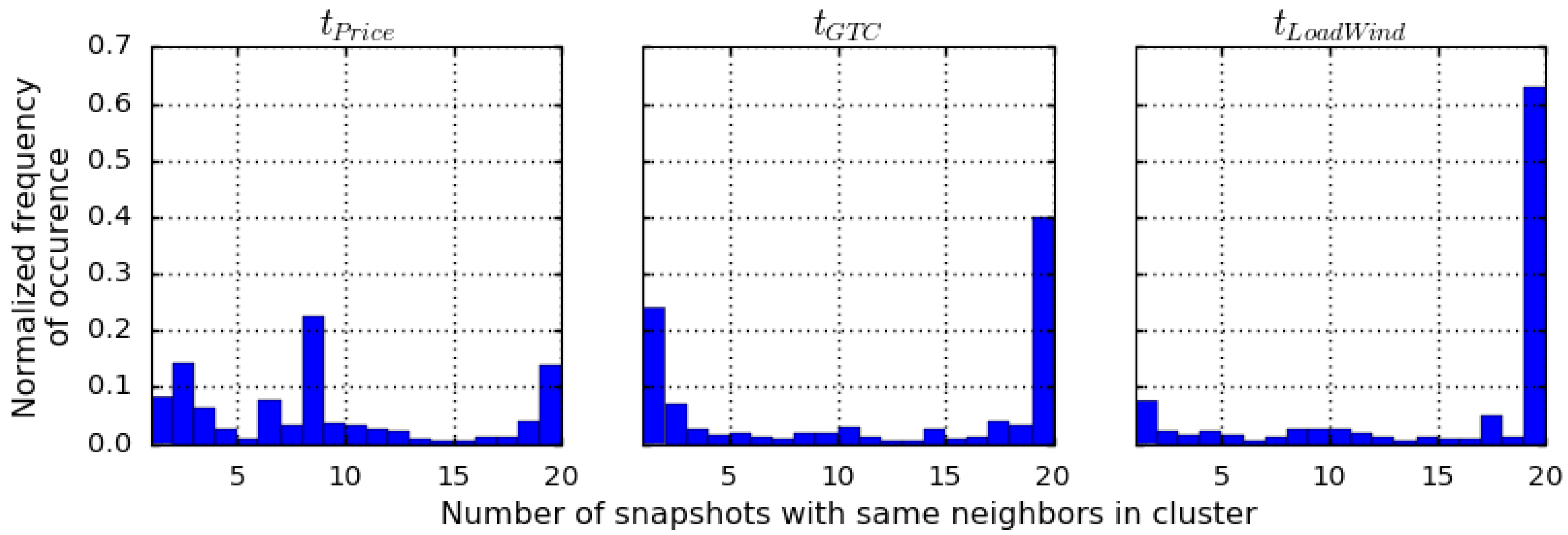
Table A1.
Applied mapping approach for the assignment of power generation and consumption to substations of the used transmission grid dataset.
Table A1.
Applied mapping approach for the assignment of power generation and consumption to substations of the used transmission grid dataset.
| Input Parameter | Approach |
|---|---|
Installed capacity of central power plants:
| Nearest neighbor |
Installed capacity of decentral power plants:
| 3-nearest neighbor |
| Annual electricity demand | 3-nearest neighbor |
Appendix C. Estimation of the Transmission Capacities from Thermal Limits
The applied transmission grid dataset contains information about the voltage level as well as the number of circuits . For an estimation of grid transfer capacities , the thermal limits of overhead transmission lines need to be known. These limits can be derived from the type of conductors installed per bundle [60]. In order to consider somehow the (n-1)-criterion as well as the fact that the calculated transmission limit for complex power in Equation (A4) needs to be higher than the required upper bound for active power flow in the model, a security margin is taken into account:
- : nominated voltage of a transmission system
- thermal limit for 243-A1/39-St1A conductors
- number of conductors per line
- number of circuits per trace
- (n-1) security margin
For the selection of an appropriate conductor type applied to all HVAC transmission lines of the grid dataset, a calibration is conducted in advance.
Appendix D. Determination of Snapshots
For spatially aggregating the results of the reference model to identify certain hours of the year as snapshots, a statistical measure is applied over the set of links or the set of nodes in the original network. For this purpose, quantiles are used instead of maximum or minimum values to avoid an overestimation of regionally limited extreme situations. The following formulas show how the points in time, that represent the snapshots which are used for executing the above presented clustering approach, are determined.
- 0.95-quantile
- Spatially aggregated time series of power generation by wind turbines and power consumption
- Time series of power generation of wind turbines in each region n
- Time series of power consumption in each region n
Spatially aggregated time series of power generation by wind turbines and power consumption
- 0.05-quantile
- Spatially aggregated time series of relative power flows
- Time series of relative power flows over each transmission line l
Appendix E. Calculation of Annual Redispatch for the Reference Model
For calculating the amount of annually redispatched power generation in a nodal pricing model, the following processing of the model results is conducted. We subtract the technology specific annual power generation of the copper plate model from the spatially summed power generation for each technology of the reference model. The result is a power balance that shows which technologies generate more or less electricity due to the consideration of power flow constraints. The annual redispatch is than observed by subtracting the power transmission losses (which do not occur in the copper plate model) either from the sum of positive values or the sum of negative values in this balance, e.g.,:
Annually redispatched energy
Appendix F. Clustering Maps
Figure A1 shows maps of Germany where substations (regions of the reference model) are same colored if they belong to the same cluster. The thick lines between the colored dots represent transmission lines that are maintained after performing the network reduction.
Figure A1.
Maps of the German electricity transmission grid model after applying the presented clustering approach based on the validation data set and different snapshot selection criteria (top) , (middle) (bottom) .
Figure A1.
Maps of the German electricity transmission grid model after applying the presented clustering approach based on the validation data set and different snapshot selection criteria (top) , (middle) (bottom) .


Appendix G. Concurrency of Redispatch Measures
To give an example of when the redispatch for different aggregated model instances (Figure 7) takes place, Figure A2 shows the curtailment of one specific technology for a selected period of time. Given that the curtailment of wind offshore power generation is caused by transmission grid congestions, it can be presumed that the points in time, when the curtailment takes place, correspond to the hours of the year when redispatch measures would occur.
Figure A2.
Curtailed power generation of wind offshore turbines for different aggregated ESM instances.
Figure A2.
Curtailed power generation of wind offshore turbines for different aggregated ESM instances.

From Figure A2 we deduce the following:
- As it could be expected, in case of the copper plate model no curtailment can be observed since no power transmission limits are considered in this aggregated ESM instance.
- The reference model (black curve) shows the highest magnitudes while the aggregated ESM instances (colored curves) underestimate these effects. However, the ESM instances determined with the spectral clustering of nodal price differences (blue curves) are closer to the reference than it is the case for the aggregated benchmark models (red curves). This corresponds to the findings deduced from Figure 7.
- The frequency of the occurrence of non-zero values in Figure A2 gives an indication for the points in time when redispatch takes place. If the colored curves show this behavior, the black curve indicates non-zero values as well. On other words, the aggregated models are able to detect curtailment or redispatch events like the reference model. This is more often the case for the blue curves than for the red ones (e.g., in hour 8132). We therefore conclude once again, that Clustered , Clustered , and Clustered perform better than the benchmark cases. However, it must be noted that they are not able to capture all relevant curtailment events of the reference model (e.g., between hours 8408 and 8456).
Appendix H. Expansion Planning in the Case Study
For performing the expansion planning study, additional constraints are taken into account which determine the investment costs for a particular technology. For example, in the case of the expansion of GTCs in the AC transmission grid, they are calculated as follows:
- Specific investment costs for AC grid expansion
- Annuity factor
In this context, Table A2 shows the used cost parameters for all technologies for which expansion planning is enabled in the case study.
Table A2.
Cost parameters for expansion planning of lithium-ion storage and grid transfer capacities.
Table A2.
Cost parameters for expansion planning of lithium-ion storage and grid transfer capacities.
| Technology | Specific Investment Costs | Life Time (Years) |
|---|---|---|
| Lithium-ion batteries | 225 €/kWh | 22 |
| GTCAC | 346 €/(km∙MW) | 40 |
| GTCDC | 544 €/(km∙MW) | 40 |
| Converter station DC | 102,000 €/MW | 20 |
References
- Paltsev, S. Energy scenarios: The value and limits of scenario analysis. Wiley Interdiscip. Rev. Energy Environ. 2017, 6. [Google Scholar] [CrossRef]
- Grunwald, A. Energy futures: Diversity and the need for assessment. Futures 2011, 43, 820–830. [Google Scholar] [CrossRef]
- Herbst, A.; Toro, F.; Reitze, F.; Jochem, E. Introduction to energy systems modelling. Swiss J. Econ. Stat. 2012, 148, 111–135. [Google Scholar] [CrossRef]
- Connolly, D.; Lund, H.; Mathiesen, B.V.; Leahy, M. A review of computer tools for analysing the integration of renewable energy into various energy systems. Appl. Energy 2010, 87, 1059–1082. [Google Scholar] [CrossRef]
- Schlachtberger, D.P.; Brown, T.; Schramm, S.; Greiner, M. The benefits of cooperation in a highly renewable European electricity network. Energy 2017, 134, 469–481. [Google Scholar] [CrossRef] [Green Version]
- Gils, H.C.; Scholz, Y.; Pregger, T.; de Tena, D.L.; Heide, D. Integrated modelling of variable renewable energy-based power supply in Europe. Energy 2017, 123, 173–188. [Google Scholar] [CrossRef]
- Pfenninger, S.; Hawkes, A.; Keirstead, J. Energy systems modeling for twenty-first century energy challenges. Renew. Sustain. Energy Rev. 2014, 33, 74–86. [Google Scholar] [CrossRef]
- Kondziella, H.; Bruckner, T. Flexibility requirements of renewable energy based electricity systems—A review of research results and methodologies. Renew. Sustain. Energy Rev. 2016, 53, 10–22. [Google Scholar] [CrossRef]
- Krishnan, V.; Ho, J.; Hobbs, B.F.; Liu, A.L.; McCalley, J.D.; Shahidehpour, M.; Zheng, Q.P. Co-optimization of electricity transmission and generation resources for planning and policy analysis: Review of concepts and modeling approaches. Energy Syst. 2015. [Google Scholar] [CrossRef]
- Haas, J.; Cebulla, F.; Cao, K.; Nowak, W.; Palma-Behnke, R.; Rahmann, C.; Mancarella, P. Challenges and trends of energy storage expansion planning for flexibility provision in low-carbon power systems—A review. Renew. Sustain. Energy Rev. 2017, 80, 603–619. [Google Scholar] [CrossRef]
- Schmid, E.; Knopf, B. Quantifying the long-term economic benefits of European electricity system integration. Energy Policy 2015, 87, 260–269. [Google Scholar] [CrossRef] [Green Version]
- Spiecker, S.; Weber, C. The future of the European electricity system and the impact of fluctuating renewable energy—A scenario analysis. Energy Policy 2014, 65, 185–197. [Google Scholar] [CrossRef]
- Lumbreras, S.; Ramos, A. The new challenges to transmission expansion planning. Survey of recent practice and literature review. Electr. Power Syst. Res. 2016, 134, 19–29. [Google Scholar] [CrossRef]
- Wang, S.J.; Shahidehpour, S.M.; Kirschen, D.S.; Mokhtari, S.; Irisarri, G.D. Short-term generation scheduling with transmission and environmental constraints using an augmented Lagrangian relaxation. IEEE Trans. Power Syst. 1995, 10, 1294–1301. [Google Scholar] [CrossRef] [Green Version]
- Zerrahn, A.; Schill, W.-P. Long-run power storage requirements for high shares of renewables: Review and a new model. Renew. Sustain. Energy Rev. 2017, 79, 1518–1534. [Google Scholar] [CrossRef]
- Göransson, L.; Johnsson, F. Cost-optimized allocation of wind power investments: A Nordic-German perspective. Wind Energy 2012, 16, 587–604. [Google Scholar] [CrossRef]
- Bucksteeg, M.; Trepper, K.; Weber, C. Impacts of renewables generation and demand patterns on net transfer capacity: Implications for effectiveness of market splitting in Germany. IET Gener. Transm. Distrib. 2015, 9, 1510–1518. [Google Scholar] [CrossRef]
- Pedregosa, F.; Varoquaux, G.; Gramfort, A.; Michel, V.; Thirion, B.; Grisel, O.; Blondel, M.; Prettenhofer, P.; Weiss, R.; Dubourg, V.; et al. Scikit-learn: Machine Learning in Python. J. Mach. Learn. Res. 2011, 12, 2825–2830. [Google Scholar]
- Moeller, C.; Meiss, J.; Mueller, B.; Hlusiak, M.; Breyer, C.; Kastner, M.; Twele, J. Transforming the electricity generation of the Berlin–Brandenburg region, Germany. Renew. Energy 2014, 72, 39–50. [Google Scholar] [CrossRef]
- Kurzidem, M.J. Analysis of Flow-Based Market Coupling in Oligopolistic Power Markets; ETH Zurich: Zürich, Switzerland, 2010. [Google Scholar]
- Anderski, T.; Surmann, Y.; Stemmer, S.; Grisey, N.; Momo, E.; Leger, A.-C.; Betraoui, B.; Roy, P.V. Modular Development Plan of the Pan-European Transmission System 2050—European Cluster Model of the Pan-European Transmission Grid; e-Highway2050: Brussels, Belgium, 2014. [Google Scholar]
- German Transmission System Operators. Übersicht über die Voraussichtliche Entwicklung der Installierten Kraftwerksleistung und der Leistungsflüsse in den Netzgebieten der Deutschen Übertragungsnetzbetreiber (Regionenmodell Stromtransport 2013); EnBW Transportnetze AG: Karlsruhe, Germany; RWE Transportnetz Strom GmbH: Dortmund, Deutschland; Transpower Stromübertragungs GmbH: Bayreuth, Deutschland; Vattenfall Europe Transmission GmbH: Berlin, Germany, 2013. [Google Scholar]
- Shayesteh, E.; Hamon, C.; Amelin, M.; Söder, L. REI method for multi-area modeling of power systems. Int. J. Electr. Power Energy Syst. 2014, 60, 283–292. [Google Scholar] [CrossRef]
- Lumbreras, S.; Banez-Chicharro, F.; Pache, C. Modular Development Plan of the Pan-European Transmission System 2050—Enhanced Methodology to Define Optimal Grid Architectures for 2050; e-Highway2050: Brussels, Belgium, 2015. [Google Scholar]
- Singh, H.K.; Srivastava, S.C. A reduced network representation suitable for fast nodal price calculations in electricity markets. In Proceedings of the IEEE Power Engineering Society General Meeting, San Francisco, CA, USA, 16 June 2005. [Google Scholar]
- Shi, D.; Tylavsky, D.J. A Novel Bus-Aggregation-Based Structure-Preserving Power System Equivalent. IEEE Trans. Power Syst. 2015, 30, 1977–1986. [Google Scholar] [CrossRef]
- Gang, L.; Dongyuan, S.; Jinfu, C.; Xianzhong, D. Automatic identification of transmission sections based on complex network theory. IET Gener. Transm. Distrib. 2014, 8, 1203–1210. [Google Scholar] [CrossRef]
- Papaemmanouil, A.; Andersson, G. On the reduction of large power system models for power market simulations. In Proceedings of the 17th Power Systems Computation Conference (PSCC), Stockholm, Sweden, 22–26 August 2011; pp. 1308–1313. [Google Scholar]
- Akhavein, A.; Firuzabad, M.F.; Billinton, R.; Farokhzad, D. Review of reduction techniques in the determination of composite system adequacy equivalents. Electr. Power Syst. Res. 2010, 80, 1385–1393. [Google Scholar] [CrossRef]
- Dorfler, F.; Bullo, F. Kron Reduction of Graphs with Applications to Electrical Networks. IEEE Trans. Circuits Syst. I Regul. Pap. 2013, 60, 150–163. [Google Scholar] [CrossRef]
- Cheng, X.; Overbye, T.J. PTDF-based power system equivalents. IEEE Trans. Power Syst. 2005, 20, 1868–1876. [Google Scholar] [CrossRef]
- Hamon, C.; Shayesteh, E.; Amelin, M.; Söder, L. Two partitioning methods for multi-area studies in large power systems. Int. Trans. Electr. Energy Syst. 2015, 25, 648–660. [Google Scholar] [CrossRef]
- Wiegmans, B. GridKit Extract of ENTSO-E Interactive Map; Zenodo: Oldenburg, Germany, 2016. [Google Scholar] [CrossRef]
- Scholz, Y.; Gils, H.C.; Pietzcker, R.C. Application of a high-detail energy system model to derive power sector characteristics at high wind and solar shares. Energy Econ. 2017, 64, 568–582. [Google Scholar] [CrossRef]
- Gils, H.C.; Simon, S. Carbon neutral archipelago—100% renewable energy supply for the Canary Islands. Appl. Energy 2017, 188, 342–355. [Google Scholar] [CrossRef]
- Gils, H.; Simon, S.; Soria, R. 100% Renewable Energy Supply for Brazil—The Role of Sector Coupling and Regional Development. Energies 2017, 10, 1859. [Google Scholar] [CrossRef]
- Gils, H.C.; Bothor, S.; Genoese, M.; Cao, K.-K. Future security of power supply in Germany—The role of stochastic power plant outages and intermittent generation. Int. J. Energy Res. 2018. accepted for publication. [Google Scholar] [CrossRef]
- Cebulla, F.; Naegler, T.; Pohl, M. Electrical energy storage in highly renewable European energy systems: Capacity requirements, spatial distribution, and storage dispatch. J. Energy Storage 2017, 14, 211–223. [Google Scholar] [CrossRef]
- Scholz, Y. Renewable Energy Based Electricity Supply at Low Costs: Development of the REMix Model and Application for Europe. Ph.D. Thesis, Universität Stuttgart, Stuttgart, Germany, 2012. [Google Scholar]
- Rippel, K.M.; Preuß, A.; Meinecke, M.; König, R. Netzentwicklungsplan 2030 Zahlen Daten Fakten; German Transmission System Operators: Brussels, Belgium, 2017. [Google Scholar]
- Teruel, A.G. Perspestective of the Energy Transition: Technology Development and Investments under Uncertainty; Technical University of Munich: Munich, Germany, 2015. [Google Scholar]
- Egerer, J.; Gerbaulet, C.; Ihlenburg, R.; Kunz, F.; Reinhard, B.; von Hirschhausen, C.; Weber, A.; Weibezahn, J. Electricity Sector Data for Policy-Relevant Modeling: Data Documentation and Applications to the German and European Electricity Markets; Data Documentation; DIW: Berlin, Germany, 2014. [Google Scholar]
- Open Power System Data Data Package Time Series. (Primary Data from Various Sources, for a Complete List See URL), Version 2017-07-09. Available online: https://data.open-power-system-data.org/time_series/2017-07-09 (accessed on 21 July 2017).
- Hörsch, J.; Brown, T. The role of spatial scale in joint optimisations of generation and transmission for European highly renewable scenarios. In Proceedings of the 2017 14th International Conference on the European Energy Market (EEM), Dresden, Germany, 6–9 June 2017; pp. 1–7. [Google Scholar]
- ENTSO-E Transparency Platform Cross-Border Commercial Schedule and Cross-Border Physical Flow. Available online: https://transparency.entsoe.eu/content/static_content/Static%20content/legacy%20data/legacy%20data2012.html (accessed on 29 June 2017).
- Eurostat European Commission Eurostat. NUTS—Nomenclature of Territorial Units for Statistics; European Commission: Brussels, Belgium, 2017. [Google Scholar]
- Bundesnetzagentur Kraftwerksliste zu der Genehmigung des Szenariorahmens für die Netzentwicklungspläne Strom 2017–2030; Bundesnetzagentur: Bonn, Germany, 2017.
- von Luxburg, U. A tutorial on spectral clustering. Stat. Comput. 2007, 17, 395–416. [Google Scholar] [CrossRef] [Green Version]
- Metzdorf, J. Development and Implementation of a Spatial Clustering Approach Using a Transmission Grid Energy System Model. Ph.D. Thesis, University of Stuttgart, Stuttgart, Germany, 2016. [Google Scholar]
- Pape, C.; Hagemann, S.; Weber, C. Are fundamentals enough? Explaining price variations in the German day-ahead and intraday power market. Energy Econ. 2016, 54, 376–387. [Google Scholar] [CrossRef] [Green Version]
- Grote, F.; Maaz, A.; Drees, T.; Moser, A. Modeling of electricity pricing in European market simulations. In Proceedings of the 2015 12th International Conference on the European Energy Market (EEM), Lisbon, Portugal, 20–22 May 2015; pp. 1–5. [Google Scholar]
- Bundesnetzagentur. Monitoringbericht 2013; Bundesnetzagentur: Bonn, Germany, 2014. [Google Scholar]
- Zhu, J. Optimization of Power System Operation; John Wiley & Sons: Hoboken, NJ, USA, 2015; Volume 47. [Google Scholar]
- ENTSO-E. Memo 2012, Provisional Values as of 30 April 2013; ENTSO-E: Brussels, Belgium, 2013. [Google Scholar]
- Zelnik-Manor, L.; Perona, P. Self-tuning spectral clustering. In Advances in Neural Information Processing Systems; The MIT Press: Cambridge, MA, USA, 2005; pp. 1601–1608. [Google Scholar]
- Breuer, C.; Moser, A. Optimized bidding area delimitations and their impact on electricity markets and congestion management. In Proceedings of the 11th International Conference on the European Energy Market (EEM14), Kraków, Poland, 28–30 May 2014; pp. 1–5. [Google Scholar]
- Mohapatra, S.; Jang, W.; Overbye, T.J. Equivalent Line Limit Calculation for Power System Equivalent Networks. IEEE Trans. Power Syst. 2014, 29, 2338–2346. [Google Scholar] [CrossRef]
- Pfenninger, S. Dealing with multiple decades of hourly wind and PV time series in energy models: A comparison of methods to reduce time resolution and the planning implications of inter-annual variability. Appl. Energy 2017, 197, 1–13. [Google Scholar] [CrossRef]
- Cao, K.-K.; Gleixner, A.; Miltenberger, M. Methoden zur Reduktion der Rechenzeit linearer Optimierungsmodelle in der Energiewirtschaft? Eine Performance-Analyse. In Proceedings of the 14th Symposium Energieinnovation, Graz, Austria, 10–12 February 2016. [Google Scholar]
- Oeding, D.; Oswald, B.R. Elektrische Kraftwerke und Netze; Springer: Berlin, Germany, 2011; ISBN 9783642192456. [Google Scholar]
Figure 1.
Possible applications of the presented method—examples of data processing using spatially aggregated energy system models (ESMs) for capacity expansion studies, (left) stochastic expansion planning, e.g., for a certain scenario year; (right) iterative expansion planning, e.g., over a period of scenario years.

Figure 2.
Clustering process, data in white boxes, processes in grey boxes.

Figure 3.
Results of the reference model validation based on a time series of daily electricity prices.
Figure 3.
Results of the reference model validation based on a time series of daily electricity prices.

Figure 4.
Duration curves of relative grid transfer capacity usage (0.95-quantile over all transmission links).
Figure 4.
Duration curves of relative grid transfer capacity usage (0.95-quantile over all transmission links).

Figure 5.
Neighborhood of 10 randomly selected regions after application of clustering based on different criteria: (left) ; (middle) ; (right) , evaluated for 20 snapshots per criterion.
Figure 5.
Neighborhood of 10 randomly selected regions after application of clustering based on different criteria: (left) ; (middle) ; (right) , evaluated for 20 snapshots per criterion.

Figure 6.
Frequency of occurrence that shows how often two regions are part of the same cluster when applying the clustering 20 times for different criteria, (left) ; (middle) ; (right) .
Figure 6.
Frequency of occurrence that shows how often two regions are part of the same cluster when applying the clustering 20 times for different criteria, (left) ; (middle) ; (right) .

Figure 7.
Redispatched power generation, relative deviation from the reference model for different aggregated ESM instances.
Figure 7.
Redispatched power generation, relative deviation from the reference model for different aggregated ESM instances.

Figure 8.
Capacity factors, relative deviations from the reference model for different aggregated ESM instances.
Figure 8.
Capacity factors, relative deviations from the reference model for different aggregated ESM instances.

Figure 9.
Utilization of transmission lines in the reference model including clustering information (colored dots) for an aggregation based on .
Figure 9.
Utilization of transmission lines in the reference model including clustering information (colored dots) for an aggregation based on .

Figure 10.
Capacity expansion for lithium-ion batteries and grid transfer capacities in different aggregated models.
Figure 10.
Capacity expansion for lithium-ion batteries and grid transfer capacities in different aggregated models.

Table 1.
Model fact sheet of the applied configuration of REMix.
| Model Name | REMix | |||
|---|---|---|---|---|
| Author (Institution) | German Aerospace Center (DLR), Institute of Engineering Thermodynamics | |||
| Model type | Linear programing Minimization of total costs for system operation Economic dispatch Optimal direct current (DC) power flow (Appendix A) | |||
| Sectoral focus | Electricity | |||
| Geographical focus | Germany | |||
| Spatial resolution | >450 nodes (reference model) | |||
| Analyzed year (scenario) | 2012 (2030) | |||
| Temporal resolution | 8760 time steps (hourly) | |||
| Input-parameters: | TM | TC | SP | |
| Conversion efficiencies [41] | √ | |||
| Operational costs [41] | √ | |||
| Fuel prices and emission allowances [42] | √ | |||
| Electricity load profiles [43] | √ | √ | ||
| Capacities of power generation, storage and grid transfer capacities and annual electricity demand [33,40,44] | √ | √ | ||
| Renewable energy resources feed-in profiles | √ | √ | √ | |
| Import and export time series for cross-border power flows [45] | √ | √ | ||
| Evaluated output parameters for clustering | Marginal costs of total power supply | √ | ||
| (Nodal balance of total power generation and consumption) | √ | |||
Table 2.
Results of reference model validation based on annual observables.
| Observed | Modeled | |
|---|---|---|
| Grid Losses [TWh] [52] | 6.2 | 5.1 |
| Redispatched energy [TWh] [52] | 2.6 | 6.65 |
| Congestion events [52] | 7160 | 17,662 |
| Annual power generation share from vRES [54] | 23% | 29% |
Table 3.
Trade-off between model accuracy and performance: objective value and total computing time for aggregated ESM instances relative to the appropriate values of the reference model (scenario data set).
Table 3.
Trade-off between model accuracy and performance: objective value and total computing time for aggregated ESM instances relative to the appropriate values of the reference model (scenario data set).
| Model Instance | Objective Value (Total System Costs) | Total Computing Time |
|---|---|---|
| Cluster & PTDF tPrice | 100.0% | 2.8% |
| Cluster & PTDF tGTC | 99.3% | 4.8% |
| Clustered tLoadWind | 98.4% | 3.9% |
| Clustered tGTC | 98.0% | 4.4% |
| Clustered tPrice | 97.6% | 3.2% |
| Simple Aggregation | 94.8% | 4.8% |
| Classical | 93.2% | 3.8% |
| Cluster & PTDF tLoadWind | 92.6% | 4.3% |
| Copper Plate | 89.8% | 0.7% |
© 2018 by the authors. Licensee MDPI, Basel, Switzerland. This article is an open access article distributed under the terms and conditions of the Creative Commons Attribution (CC BY) license (http://creativecommons.org/licenses/by/4.0/).
Share and Cite
MDPI and ACS Style
Cao, K.-K.; Metzdorf, J.; Birbalta, S. Incorporating Power Transmission Bottlenecks into Aggregated Energy System Models. Sustainability 2018, 10, 1916. https://doi.org/10.3390/su10061916
AMA Style
Cao K-K, Metzdorf J, Birbalta S. Incorporating Power Transmission Bottlenecks into Aggregated Energy System Models. Sustainability. 2018; 10(6):1916. https://doi.org/10.3390/su10061916
Chicago/Turabian StyleCao, Karl-Kiên, Johannes Metzdorf, and Sinan Birbalta. 2018. "Incorporating Power Transmission Bottlenecks into Aggregated Energy System Models" Sustainability 10, no. 6: 1916. https://doi.org/10.3390/su10061916
Note that from the first issue of 2016, this journal uses article numbers instead of page numbers. See further details here.