Spatio-Temporal Features of Urban Heat Island and Its Relationship with Land Use/Cover in Mountainous City: A Case Study in Chongqing

Abstract

The urban heat island (UHI) becomes more and more serious with the acceleration of urbanization. Many researchers have shown interest in studying the UHI by using remote sensing data, but these studies rarely examine the mountainous cities. Studies on UHI in mountainous cities often used empirical parameters to estimate the land surface temperature (LST), and lacked satellite-ground synchronous experiments to test the accuracy. This paper revised the parameters in the mono-window algorithm used to retrieve the LST according to the characteristics of mountainous cities. This study examined the spatial and temporal patterns of the UHI intensity in Chongqing, a typical mountainous city, and its relationship with land cover from 2007 to 2016 based on the Landsat 5 TM and Landsat 8 TIRS data and the improved method. The accuracy of the LST derivation increased by about 1 °C compared to the traditional method. The high LST areas increased and extended from the downtown to suburban area each year, but the rate of change decreased. The UHI is dramatically impacted by the rivers. There is a good relationship between the urban sprawl and the UHI. The LST was reduced by about 1 °C within a 300 m distance from large urban fringe green spaces. The urban landscape parks had a strong effect relieving the UHI at a 100 m distance. The LST was reduced by about 0.5 °C. This study greatly improves the accuracy of LST derivation, and provides reliable parameters for the UHI researched in mountainous cities.

1. Introduction

Urbanization is one important attribute of regional social and economic development. It results in land use/cover changes and increased building density, both horizontally and vertically, in urban areas. These changes associated with urbanization impact on urban climate considerably [1,2]. The consistent and significant increase in surface air temperature in urban areas relative to in surrounding rural areas, a phenomenon termed as urban heat island (UHI) effect, has been exacerbated [3]. At the same time, the eco-environment problems caused by UHI become more and more serious with the acceleration of urbanization [4,5]. In recent decades, UHI effects have been the focus of study of sciences, and large UHI effects have been measured and reported for most regions of the world. The UHI of New York City is performed using a mesoscale network of weather stations by Gedzelman et al. [6]. It averages about 4 °C in summer and autumn and 3 °C in winter and spring. According to Weng, urban land development raised surface radiant temperature by 13.01 K between 1989 and 1997 in Zhujiang Delta of South China. The spatial pattern of radiant temperature increase was correlated with the pattern of urban expansion [7]. Ogashawara et al. found that the distribution of UHIs in São José dos Campos has expanded rapidly from 1986 to 2010. The correlations between the Normalized Difference Vegetation Index (NDVI) and Normalized Difference Water Index (NDWI) and temperature were low (<0.5); a moderate correlation was found between the Normalized Difference Built-up Index (NDBI) and temperature [8]. Many other researchers also have shown interest in estimating the magnitude of UHI, analyzing its spatio-temporal evolution features, understanding its implication with respect to a broad set of environmental factors, and looking for the measures to reduce its detrimental effects [9,10,11,12,13,14,15,16]. These studies on the UHI phenomenon can be divided into two types: ground-based observed air temperature in urban and rural weather stations and remotely-sensed data-based land surface temperature [17]. It is well known that the air temperature defined UHI can be used to analyze the long-term trend, but considerable efforts must be made to correct air temperature biases when comparing UHI effects across different regions. It is difficult to analyze the UHI phenomenon in the regions where there are not enough weather stations. The remote sensing data with the advantages of large area, synchronization, and spatial coverage has become the effective tool for studying UHI phenomenon [18,19,20,21,22]. Rao studied the UHI effects by using thermal remote sensing data for the first time in 1972 [23]. Since then, many scientists turned to the use of remotely-sensed data for UHI effect analysis [8]. The remote sensing data, such as NOAA (National Oceanic and Atmospheric Administration), MODIS (Moderate Resolution Imaging Spectroradiometer), TM (Landsat Thematic Mapper), ETM+ (Enhanced Thematic Mapper Plus), etc., were widely used to examine the UHI effects [12,18,19]. Many algorithms for UHI based on remote sensing were also be developed by the scientists [24]. Among many UHI algorithms based on remote sensing, the mono-window algorithm, because it is easy and feasible, is widely used in the studies of UHI [9,15,22,23,24,25,26]. While these detailed studies provide an excellent basis for understanding UHI, there are also some limitations: (1) These studies rarely examined the mountainous cities; (2) Few studies on UHI in mountainous cities based on remote sensing data often used empirical parameters to estimate the land surface temperature (LST). It is therefore hampered by the lack of proper parameters to retrieve the LST in mountainous cities; (3) Many studies lacked satellite-ground synchronous experiment to test the accuracy.

Chongqing, a typical mountainous city, is located at the valley between Mount Tongluo and Mount Zhongliang. The eco-environmental problems caused by UHI are becoming increasingly acute with the acceleration of urbanization. Ren found that the UHI intensity of Chongqing increased year by year. The UHI effect was stronger in winter and at night [27]. Li et al. indicated that the UHI was contemporaneous with the Urban Wet Island (UWI) in Chongqing. The vertical structure of UHI was shown as the city being covered by warm moist air at 200–300 m above the river level [28]. He et al. discovered that the UHI was influenced by the mountainous terrain features and city layout in Chongqing [29]. Dan et al. thought that the Yangtze River and Jialing River had important effects on the UHI of Chongqing [30]. Some other scholars also did some research on UHI in Chongqing [31,32]. Although Chongqing’s UHI effect has been well studied, most of the literature is based on weather station data, which neglects the spatial extension and distribution of UHI. These studies also lack necessary verification of their precision. Furthermore, it is necessary to better understand how the impact factors, especially urban green spaces, influence the UHI effect in Chongqing.

In this study, we rectify the parameters used in the mono-window algorithm according to the terrain features of Chongqing. We use a combination of Landsat TM and Landsat 8 TIRS data, automatic weather station data, and satellite-ground synchronous experiment data to estimate the LST, test its accuracy, and examine the relationship between the impact factors and the UHI variations in Chongqing. The main objective of this study is to provide a suitable quantitative method to study UHI in mountainous cities.

2. Materials and Methods

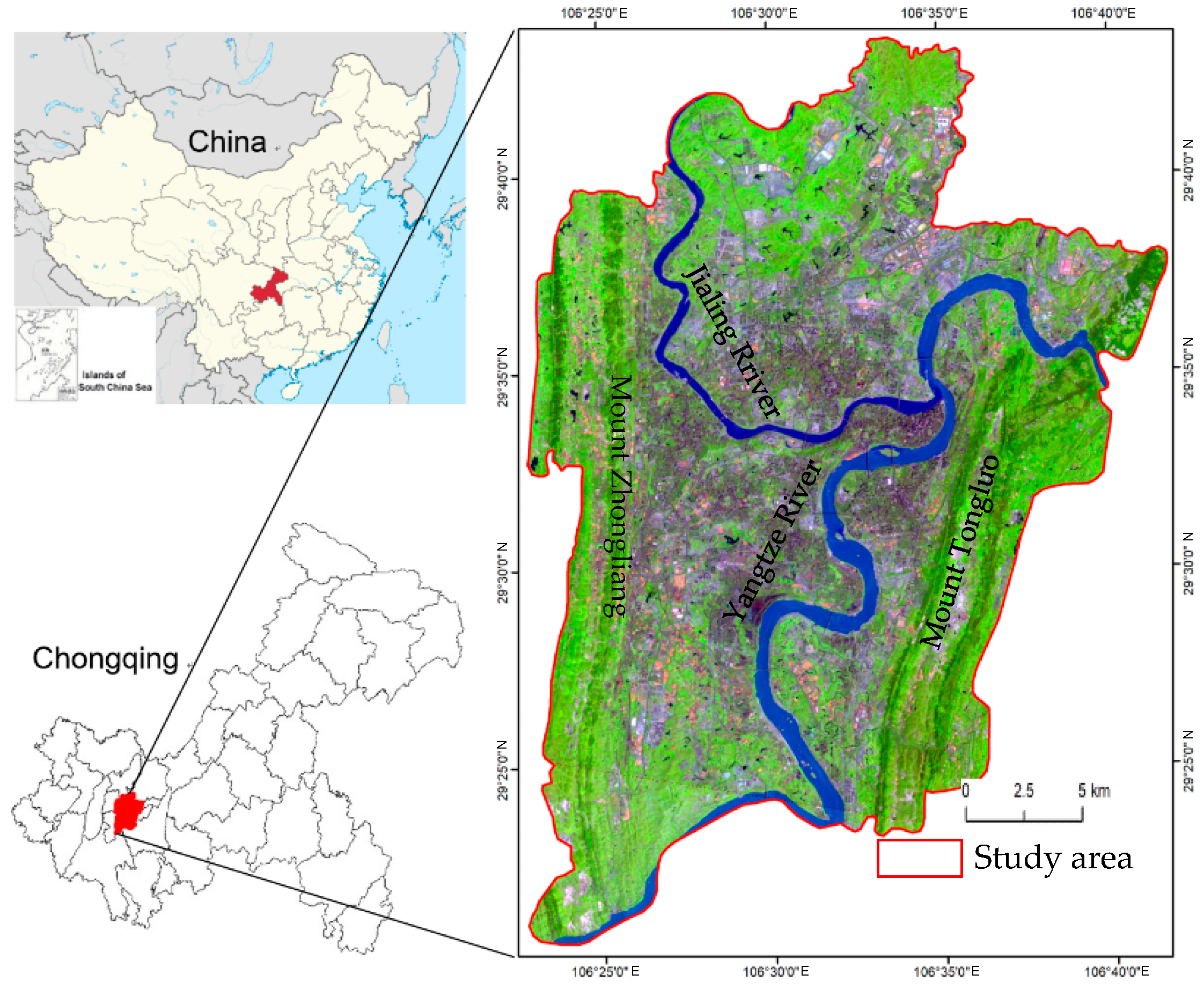
2.1. Study Area

Chongqing municipality, one of the fastest developing cities in China over the past twenty years, is situated in southwest China. Characterized by rugged hills, Chongqing is a typical mountainous city and is also one of the three famous “stoves” of China. The study area is located between 106°23′2.4″E–106°41′45.6″E and 29°20′31.2″N–29°43′26.4″N in the southwest of Chongqing municipality, with a total area of approximately 780 km² (Figure 1). It has a humid subtropical monsoon climate, and receives an average annual precipitation of 1000 mm. The average annual temperature is 18.4 °C. The Yangtze River and Jialing River go through the area roughly from south to north and from west to east respectively, uniting in the city center. Separated by the terrain and the rivers, naturally, the study area forms a multi-center structure. The UHI phenomenon in the study area is obvious because of the air circulation caused by the terrain barrier, and the high population and building density caused by rapid urbanization [33].

2.2. Data and Image Pro-Processing

Satellite remote sensing offers a great opportunity to acquire continuous LST data without direct physical contact with the surface, with sufficient spatial resolution to distinguish between urban and surrounding rural areas [34]. The Landsat 5 TM and Landsat 8 TIRS are the most widely used remote sensing data for UHI studies. Five Landsat 5 TM images (i.e., 20 September 2007; 20 July 2008; 24 September 2009; 11 August 2010 and 30 August 2011) and four Landsat 8 TIRS images (i.e., 19 August 2013; 6 August 2014; 8 July 2015 and 10 July 2016) were used for retrieval of LST in this study. The data acquisition dates had highly clear atmospheric conditions, and the images were acquired from the Institute of Remote Sensing and Digital Earth Chinese Academic of Sciences Data Center, which corrected the radiometric and geometrical distortions of the images before delivery. The images were further rectified to a common Universal Transverse Mercator coordinate system based on 1:10,000 scale topographic maps, and were resampled using the nearest neighbor algorithm with a pixel size of 30 by 30 m for all bands, including the thermal bands (with the resolution of 120 by 120 m and 100 by 100 m for Landsat 5 TM and Landsat 8 TIRS respectively). The resultant RMSE was found to be less than 0.5 pixels. In addition, the meteorological data from 4 standard weather stations, 11 intensive automatic weather stations, and 19 field observing sites, the urban planning data, the land use/cover, and some other auxiliary data were used to assist in the analysis.

The sensor TM band 6 and TIRS band 1 on Landsat 5 and Landsat 8 measures the radiances at the top of the atmosphere, and its brightness temperatures can be derived using Plank’s law [35]. The approach to the retrieval of temperature was described in the User’s Handbook. The following equation was used to convert the digital number (DN) of TIR bands into spectral radiance:

L_λ = DN (L_max − L_min)/255 + L_min,

(1)

where L_λ is spectral radiance; DN represents the digital number of band 6 of TM and band 1 of TIRS; L_max and L_min (given in the header files of the images) are the maximum and minimum spectral radiance of band 6 of TM and band 1 of TIRS respectively.

The next step is to convert the spectral radiance to at-satellite brightness temperature under the assumption of uniform emissivity. The conversion formula is:

T = K₂/ln(1 + K₁/L_λ),

(2)

where T is the effective at-satellite brightness temperature in K of band 6 of TM and band 1 of TIRS; L_λ is spectral radiance; and K₁ and K₂ are pre-launch calibration constants.

2.3. Derivation of LST and Improvement of the Parameters

The methods for the retrieval of LST from satellite TIR (Thermal Infrared) data can be broadly classified into three categories: single-channel methods, multi-channel methods (split-window algorithm, SWA), and multi-angle methods [36,37,38]. In comparison with other methods, the mono-window algorithm is simpler and only three parameters (the average atmospheric operative temperature, land surface emissivity and atmospheric transmittance) are needed; therefore, the mono-window algorithm was used to calculate the LST for the Landsat TM and TIRS images. The mono-window algorithm’s calculation formula is as follows [39]:

T_s = {a(1 – C − D) + [b(1 – C − D) + C + D]T + DT_a}/C,

(3)

where T_s is the emissivity-corrected land surface temperatures, and a and b are regression coefficients. In most studies, the values of the a and b were given roughly as −67.35535, 0.458608, respectively, within the temperature range of 0~70 °C. The images used in this study are all at noon in summer, and the range of temperature variation is small. In this case, the a and b are equal to -67.9542 and 0.45987, respectively (within the temperature range of 20~50 °C); C = τε and D = (1 − τ)[1 + τ(1 − ε)] are the intermediate variables; τ is the atmospheric transmittance; ε is the land surface emissivity; T is the effective at-satellite brightness temperature of band 6 (TM) and band 1 (TIRS); and T_a is the effective mean atmospheric temperature.

τ, ε and T_a are three essential parameters in the mono-window algorithm. Many researchers used these empirical values in their studies. But, in fact, the mono-window algorithm is sensitive to parameters. So it is obvious that the empirical values are not suitable to the retrieval of LST in Chongqing, a typical mountainous city with complex terrain features. In this study, we improved the method to estimate the three essential parameters, and the retrieval accuracy of LST was also improved.

2.3.1. Determination of the Land Surface Emissivity (ε)

The urban area can be divided into water, natural surface, and built-up. If land over is water then ε_w = 0.995. If land cover is natural surface, and NDVI < 0.05, then it is bare land, and ε_s = 0.972. If NDVI > 0.7, it is fully covered by vegetation, and ε_v = 0.986. When NDVI ϵ [0.05, 0.7], the land surface emissivity (ε) was computed as follows [19]:

ε = P_v R_vε_v + (1 − P_v) R_sε_s + d_ε,

(4)

When land cover is built-up, the land surface emissivity (ε) was computed as follows [19]:

ε = P_v R_vε_v + (1 − P_v) R_m ε_m + d_ε,

(5)

where P_v is vegetation coverage; R_v = 0.9332 + 0.0585P_v is vegetation temperature ratio; ε_v = 0.986 is land surface emissivity with very high vegetation coverage; R_m = 0.9886 + 0.1287P_v is the building surface temperature ratio; and ε_m = 0.972 is the building surface emissivity. The effect of d_ε is negligible in many studies. They all assume that the land surface is flat. As mentioned before, the terrain of Chongqing is complex. In this paper, we estimated the value of d_ε according to the vegetation coverage (when P_v ≤ 0.05, d_ε = 0.0038; when P_v > 0.05, d_ε = 0.0038(1 − P_v)).

2.3.2. Determination of Atmospheric Transmittance (τ)

The atmospheric transmittance (τ) can be estimated by the following equation [39]:

τ = 0.97429 − 0.08007ω, ω ϵ [0.4, 1.6]; τ = 1.031412 − 0.11536ω, ω ϵ [1.6, 3.0],

(6)

where ω is atmospheric water vapor content in g·cm⁻². In many studies, ω was often estimated by experience. In our study, we calculate it as follows [40]:

ω = a₀ + a₁e,

(7)

where a₀ and a₁ are empirical constants. The central latitude and average altitude of the study area are 29.5° and 350 m, respectively, so we can determine ω = 0.04691+ 0.19604e, according to Yang et al. e is absolute vapor pressure. It can be calculated as follows [40]:

e = 0.6108exp[17.27(T₀ − 273.15)/(237.3 + T₀ − 273.15)]RH,

(8)

where T₀ is air temperature, and RH is relative humidity. Due to a lack of meteorological data, most of the studies use the meteorological data from standard weather stations to estimate e. Unfortunately, urban areas often have few weather stations, making the accuracy of e unsatisfactory. In this study, the meteorological data from 4 standard weather stations, 11 intensive automatic weather stations, and 19 field observing sites are combined to determine the value of e. We therefore generated satisfactory results.

2.3.3. Determination of Effective Mean Atmospheric Temperature (T_a)

According to Qin et al. for mid-latitude summers, T_a can be approximated as [39]:

T_a = 16.011 + 0.92621T₀,

(9)

where T₀ is near-surface air temperature. In this paper, we improved the accuracy of T_a by using the integrated meteorological data from standard weather stations, intensive automatic weather stations, and field observing sites.

3. Results

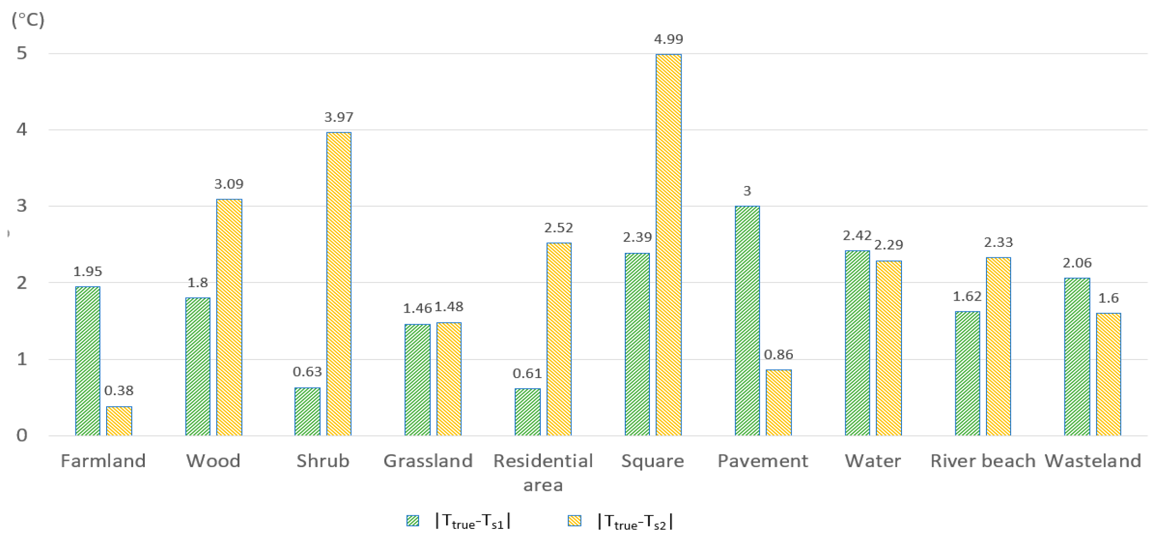
3.1. Retrieval Accuracy Validation of LST Based on Satellite-Ground Synchronous Experiment

The best way to validate retrieval accuracy is to compare the in-situ ground truth measurements of LST with the retrieved ones from the remote sensing images data of a specific region. On 30 August 2011, we carried out a satellite–ground synchronous experiment at a Landsat TM pass over the study area. We recorded the air temperature, LST, wind speed, and air humidity at 46 field sites each 15 min from 9:30 a.m. to 3 p.m. In actual operation, we used the data from 19 sites with high reliability to validate the retrieval accuracy of LST (

Table 1. Retrieval accuracy validation of LST based on satellite-ground synchronous experiment.

Land Use/Cover	Sites	Ground Measurement LST Ttrue (°C)	Method of Improved Parameters		Method of Empirical Parameters
			Retrieved LST Ts1 (°C)	Absolute Difference |Tture − Ts1| (°C)	Retrieved LST Ts2 (°C)	Absolute Difference |Ttrue − Ts2| (°C)
Farmland	Yuanyuang	35.20	37.15	1.95	34.82	0.38
Wood	Nanshan	36.00	35.83	0.17	31.95	4.05
Wood	Zhaomushan	26.50	29.20	2.70	27.69	1.19
Wood	Shaping	34.00	34.20	0.20	30.47	3.53
Wood	Huahui	37.70	34.10	3.60	32.98	4.72
Wood	Pingtingshan	31.00	33.33	2.33	29.02	1.98
Shrub	Guanyinqiao	39.90	39.27	0.63	35.93	3.97
Grassland	Chaotianmen	36.00	36.85	0.85	33.09	2.91
Grassland	Bailin	31.00	33.06	2.06	31.05	0.05
Residential area	Houbao	35.10	35.71	0.61	32.58	2.52
Square	Longtousi	37.20	36.92	0.28	33.57	3.63
Square	Caiyuanba	42.50	39.84	2.66	37.42	5.08
Square	Dachuan	43.20	38.98	4.22	36.95	6.25
Pavement	Jinyuan	27.00	30.00	3.00	26.14	0.86
River beach	Jialing river 1	29.10	30.57	1.47	26.16	2.94
River beach	Yangtze river 1	27.00	28.77	1.77	28.72	1.72
Water	Jialing river 2	28.50	30.57	2.07	32.57	4.07
Water	Yangtze river 2	26.00	28.77	2.77	26.5	0.50
Wasteland	Dadukou	36.50	38.56	2.06	34.90	1.60
Mean	-	33.65	34.30	1.86	31.71	2.73

).

The results in Table 1 indicate that the LSTs retrieved after improving the parameters are generally higher than the in-situ ground truth measurements of LSTs. The mean values are 34.30 °C and 33.65 °C, respectively, with a difference of 0.65 °C. The maximum, minimum, and mean absolute difference between T_true and T_s1 are 4.22 °C, 0.17 °C, and 1.86 °C. We also compared the retrieved LST by comparing the empirical parameters with the ground truth LST. The former is generally lower than the latter. The mean value is lower by 1.94 °C. The maximum, minimum, and mean absolute difference between T_true and T_s2 are 5.08 °C, 0.05 °C, and 2.73 °C. The retrieval accuracy of LST in different land use/cover types are shown in Figure 2. The results suggest that the method of improved parameters has higher accuracy in wood, shrub, residential area, square, and river beach than in the method of empirical parameters. In farmland and pavement, the method of improved parameters shows a lower LST retrieval accuracy. On the whole, the experimental results show that the LSTs retrieved by using the improved parameters are more accurate compared to the LSTs retrieved based on the previous parameters. This good matching of the LSTs retrieved to the actual ones confirms the applicability of the improved parameters to the UHI studies in mountainous cities.

LST images from nine periods Landsat 5 TM6 and Landsat 8 TIRS1 data of the study area were calculated using the improved parameters mono-window algorithm (Figure 3,

Table 2. LSTs of the nine dates (°C).

Date	LSTmin	LSTmax	LSTmean	LSTstd
20 September 2007	28.63	56.90	36.71	2.02
20 July 2008	26.00	44.64	33.24	2.02
24 August 2009	28.43	50.22	35.04	2.25
11 September 2010	25.44	47.20	34.01	2.24
30 August 2011	26.28	51.26	37.00	2.78
19 August 2013	25.32	48.21	34.89	2.40
6 August 2014	25.98	52.79	34.90	2.33
8 July 2015	24.98	46.58	31.24	2.34
10 July 2016	28.01	46.52	34.61	2.20

). In order to eliminate the effects of the environmental factors, we normalized the LSTs to 0~1, and divided them to seven levels (i.e., very high temperature area, high temperature area, sub-high temperature area, medium temperature area, sub-medium temperature area, low temperature area, and very low temperature area) by using the natural breaks grading method (Figure 4,

Table 3. The area ratio of different LST levels from 2007 to 2016 (%).

Level	20 September 2007	20 July 2008	24 August 2009	11 August 2010	30 August 2011	19 August 2013	8 August 2014	8 July 2015	10 July 2016
Very low LST	4.24	4.32	5.04	3.45	2.61	4.12	12.16	12.25	4.28
Low LST	49.37	23.17	41.33	4.65	7.23	38.93	35.71	39.65	40.41
Sub-medium LST	44.29	59.77	42.65	36.93	54.99	33.39	31.10	34.16	44.67
Medium LST	1.96	12.24	10.02	47.65	32.04	16.20	11.72	9.38	7.75
Sub-high LST	0.11	0.55	0.86	7.02	2.96	6.96	8.69	3.76	2.64
High LST	0.02	0.04	0.09	0.28	0.16	0.37	0.55	0.77	0.24
Very high LST	0.01	0.00	0.01	0.02	0.01	0.03	0.07	0.03	0.01
Sum of high and very high LST	0.03	0.04	0.10	0.30	0.17	0.40	0.62	0.80	0.25

).

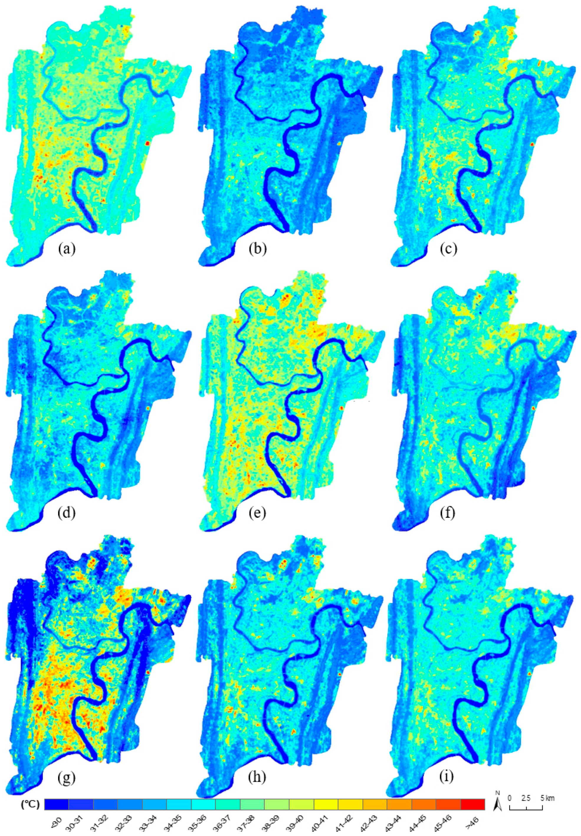
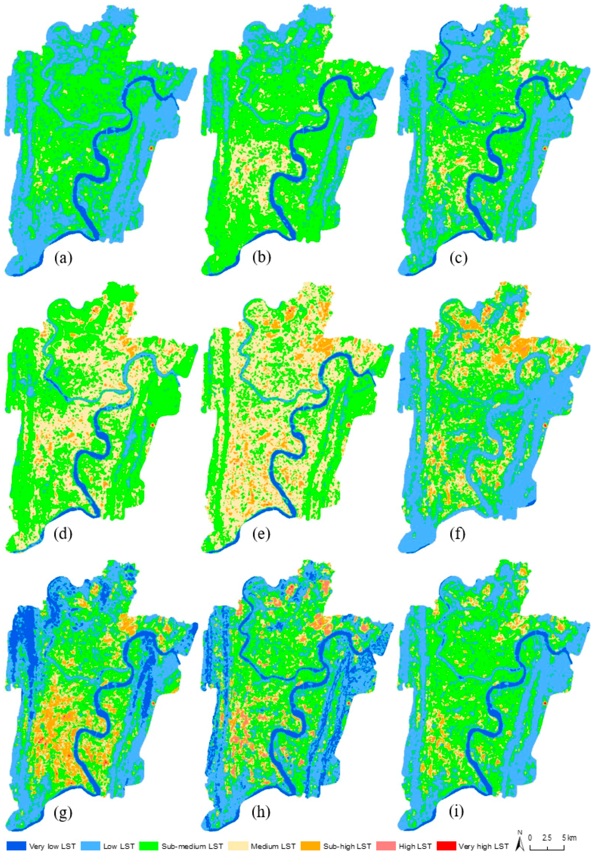
3.2. Spatio-Temporal Features of UHI

The temporal variation and spatial distribution of annual UHI over the study area are shown in Figure 3 and Figure 4, Table 2 and Table 3. The results suggest that The LSTs show a gradually increasing trend from 2007 to 2011, and a decreasing trend from 2011 to 2016. The spatial pattern of the UHI changed from a scattered pattern in 2007 to a more contiguous pattern in 2011 and 2016, along with the expansion of the regional urban system. The centers of high temperature were consistent with built-up and bare land areas, and the low-temperature centers are located in the area of two rivers (i.e., Yangtze River and Jialing River) and two mountains area (i.e., Mount Zhongliang and Mount Tongluo). The relatively high temperature areas (i.e., very high LST area and high LST area) shifted from south to north and expand from the central city to the outskirts. On 20 August 2011, the mean LST was 37 °C. In most of the study area, the LST was above 35 °C, and the maximum LST was even up to 51.26 °C. Compared to 2007, the mean LST increased by 0.29 °C, the distribution of the relatively high temperature areas became more even. The minimum LST was 28.01 °C, and the maximum LST was 46.52 °C on 10 July 2016. Compared to 2011, the mean LST decreased by 2.39 °C. The distribution of high-temperature centers was more disperse from 2007 to 2016, and their inner structure and composition obviously changed. These distributions and changes of the UHI effect are closely related to the types and functions of the different underlying surface and their changes.

In the study area, the very low LST areas were mainly the large water bodies, such as ponds, reservoirs and rivers, and changed with the water level. There were marked changes from 2007 to 2016, and the area ratio showed an obvious increasing trend from 2007 to 2016. (Table 3). The low LST areas concentrated on the high vegetation coverage areas and some small water bodies. After 2009, the area ratio sharply decreased, while it increased quickly from 2011 to 2013. Then, the increasing trend slowed down. The sub-medium LST areas were located in the sub-high vegetation coverage areas and farmlands. They changed in volatility from 2007 to 2016. The medium LST areas were the forests and grasslands with low vegetation coverage and some farmlands, and increased rapidly over time, from 15.29 km² in 2007 to 371.79 km² in 2010. The medium LST area ratio decreased quickly from 2010 to 2016. The high LST areas, and very high LST areas were mainly distributed in the industry lands, built-up areas, and development and construction areas. Compared to 2007, the total area ratio of the two types quickly increased as a general trend and was up to 0.80%, and 0.25%, respectively in 2015 and 2016. The relatively high temperature areas were spotty and distributed linearly in 2007, and the large high temperature areas were mainly located in the business and industry concentrating areas, such as Yuzhong, Dadukou, and Jiulongpo, etc. In 2008, the relatively high temperature areas also distributed in the business and industry centers within the inner ring road, but the spatial structure gradually transformed from a dispersedly spotty and linear distribution to continuous area distribution. At the same time, many constructing areas became the new high temperature centers. In 2009, when the lands within the inner ring road had not met the urban development, some new high temperature areas appeared outside inner ring road, such as Lianglu, Jingkou, Tangjiatuo, Lishuwan, Chonggang, Changgang, etc. The LST was generally higher in 2010. The main change in this year was the obviously northward shift of the high-temperature centers, and the expansion of the relatively high temperature areas (from 0.76 km² in 2009 to 57.07 km² in 2010). In 2011, the relatively high temperature areas decreased compared to 2010 (from 2.35 km² in 2010 to 1.31 km² in 2011), but it was still far more than it was in 2007, 2008, and 2009. Although the relatively high LST areas were largest in 2010, apparently there was a general trend of increasing UHI effect from 2007 to 2011. From 2011 to 2015, the relatively high temperature areas continually increased. The area ratio increased from 0.17% to 0.80. In 2016, the area ratio decreased to 0.25%.

3.3. Relationship between LST and NDVI

The Normalized Difference Vegetation Index (NDVI) was calculated for each image. The negative correlations were found between NDVI and LST by comparing both images. In order to further study their quantitative relationship, the NDVI and LST images on 30 August 2011 are selected as samples to establish the linear regression. Its regression equation was given as follows.

LST = −6.212NDVI + 38.89 (NDVI ≥ 0),

(10)

With the increasing of NDVI, the LST decreased from approximately 45 °C to 33 °C. When NDVI was approximately 0.18, some pixels had a higher LST. After analyzing the NDVI, LST and high-resolution images, we find that most of these pixels were in the new construction areas.

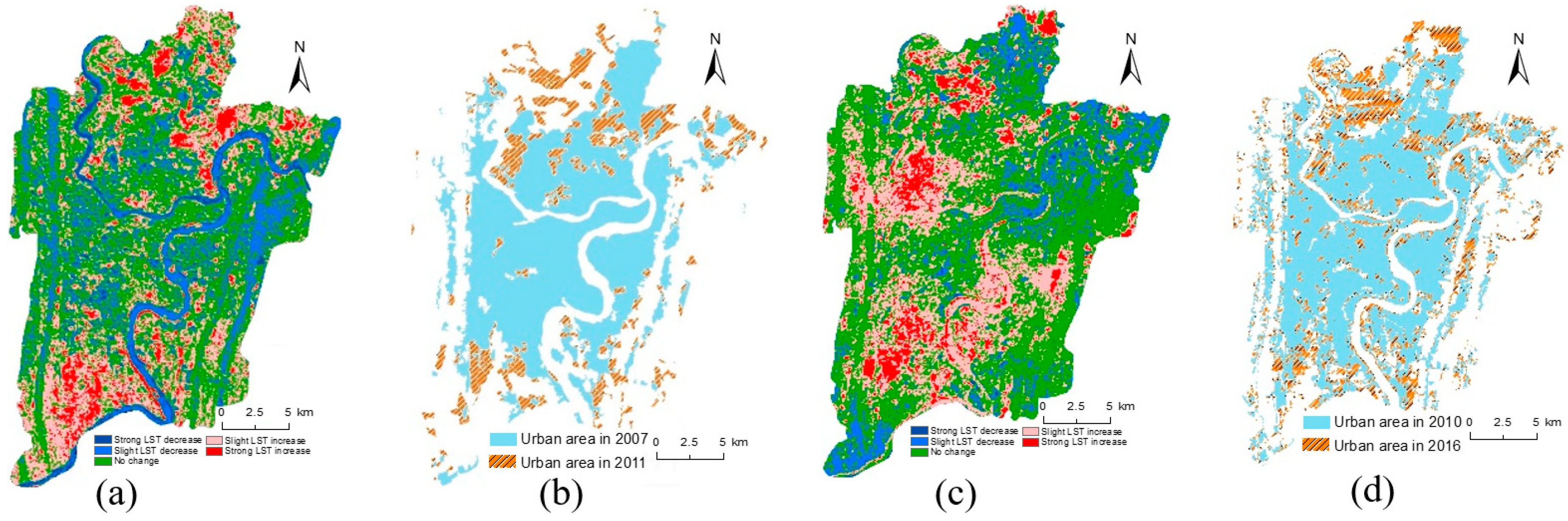
3.4. Relationship between UHI and Urban Expansion

In the paper, the LST changes were detected from 2007 to 2016, and the amplitude of changes are classified on

Table 4. Classification standard of the LST change.

Types	Strong LST Decrease	Slight LST Decrease	No Change	Slight LST Increase	Strong LST Increase
LST2011–LST2007	<−3 °C	−3–−1 °C	−1–1 °C	1–3 °C	>3 °C

, Figure 5.

In Figure 5, we find that the LST decrease areas are mainly the water bodies and high vegetation coverage areas, the no-change areas are distributed in the old urban districts, and the LST increase areas are located at the north and south of the study area. From 2007 to 2011, the urban area also mainly expanded to north and south (Figure 5b). From 2010 to 2016, the urban area expanded not only to north and south, but also to east (Figure 5d). By comparing Figure 5a with Figure 5b, and Figure 5c with Figure 5d, there is a good correlation between the expansion of urban area and UHI in pattern, position and amount. The urban area expanded by 85.9 km² from 2007 to 2011, and by 97.01 km² from 2010 to 2016. The strong LST increase areas showed a rise of 54.57 km² and 58.41 km² during the same time. It is obvious that the urban expansion was the main contributor to the UHI.

3.5. Relationship between UHI and Land Use/Cover

In this paper, we also explored the effect of different land use/cover types for UHI in a mountainous city. Five land use/cover types were classified in the study area (i.e., built-up, bare land, vegetation, water and road). Vegetation is the area containing forests, shrubs, grasslands and crops. Water includes reservoirs, ponds and rivers. The area under development is similar to bare land. The maps of land use/cover were retrieved from a Landsat images on 20 September 2007, 30 August 2011, and 10 July 2016. To study the temperature relationship of different land use/cover types, the maximum, minimum, and mean LST of different land use/cover types were derived by averaging all corresponding pixel values (

Table 5. LST in different land use/cover types in 2007, 2011 and 2016.

Land Use/Cover	Minimum LST (°C)			Maximum LST (°C)			Mean LST (°C)
	2007	2011	2016	2007	2011	2016	2007	2011	2016
Built-up	30.42	26.75	25.73	51.39	46.78	43.45	38.13	35.24	35.82
Bare land	30.03	28.72	26.45	56.9	47.20	46.52	38.37	36.91	37.27
Vegetation	29.52	28.33	25.79	48.39	40.99	41.77	36.27	33.43	30.37
Water	28.63	25.44	28.01	35.09	36.25	42.97	32.82	29.61	27.77
Road	30.05	32.81	26.03	45.11	43.49	42.32	37.7	34.82	32.74

). It can be found from Table 5 that the maximum and mean LST in bare land are all highest followed by build-up, and the maximum and mean LST in water are lowest due to its high heat capacity.

To further study the relationship between LST and land use/cover types, the areas of each LST level in different land use/cover types in 2007, 2011, and 2016 were calculated (

Table 6. Area of each LST level in different land use/cover types in 2007, 2011 and 2016 (km²).

Land Use/Cover	LST Levels
	Very Low LST			Low LST			Sub-Medium LST			Medium LST			Sub-High LST			High LST			Very High LST
	2007	2011	2016	2007	2011	2016	2007	2011	2016	2007	2011	2016	2007	2011	2016	2007	2011	2016	2007	2011	2016
Built-up	0.67	0.18	1.75	41.91	5.20	53.09	227.93	119.63	251.74	14.20	171.27	44.35	0.79	13.80	14.83	0.04	0.30	1.17	0.07	0.01	0.02
Bare land	0.00	0.00	0.00	0.18	0.34	0.19	0.55	4.87	5.06	7.18	19.65	31.15	2.14	8.05	4.53	0.24	0.82	1.32	0.16	0.08	0.10
Vegetation	1.18	0.01	0.79	314.26	24.48	218.65	108.33	293.80	87.07	0.65	56.89	6.96	0.04	1.02	0.49	0.01	0.02	0.02	0.00	0.00	0.00
Water	31.29	20.18	30.48	24.39	26.27	20.04	2.70	9.96	3.69	0.04	1.14	0.19	0.05	0.17	0.02	0.02	0.08	0.04	0.00	0.00	0.00
Road	0.04	0.00	0.00	0.07	0.00	0.04	0.11	0.10	0.35	0.13	0.18	0.44	0.01	0.00	0.24	0.00	0.00	0.94	0.01	0.00	0.05

). Using the information, how the land use/cover types may have contributed to UHI can be estimated. From our analysis, it can be seen that almost all land use/cover types except water were distributed over the medium and sub-medium LST areas. The difference is that the areas of bare land and road located in medium LST areas were larger than those in sub-medium LST areas, but the vegetation was the opposite. The vegetation areas mainly showed the characteristics of low and sub-medium LST. The relatively high LST areas concentrated in the built-up (0.9 km², 14.11 km², 16.01 km²) and bare land (2.54 km², 8.95 km², 5.95 km²) in 2007, 2011, and 2016. They nearly matched the total contribution. Most of the areas of built-up were medium and sub-medium LST. However, the low and very low LST areas were highly concentrated in water and vegetation. Both of them contributed more than 90% to the total area of low and very low LST areas in the study area. So, it is easy to conclude that water and high coverage vegetation areas play an important role mitigating the UHI effect.

3.6. Mitigating Effects of Different Urban Green Spaces on UHI

Two types of urban green spaces (i.e., urban fringe forests and urban parks) were selected in the study. The urban fringe forests with large areas were retrieved from Landsat TM on 30 August 2011 (Figure 6), and the urban parks data was provided by Chongqing Park Management and Landscape Planning Bureau. The urban fringe forests include three primary parts: Mount Tongluo located in the east, Mount Zhongliang located in the west, and some hills located in the north. Nine urban parks were selected as samples in the paper (i.e., Bolin park, Dongbu park, Eling park, Huahui park, Zhongyang park, Pingdingshan park, Shaping park, Shanhu park, Shimen park). We created six buffers per 50 m for each urban fringe forest and urban park in this study and estimated the mitigating effects of these urban green spaces on UHI (

Table 7. Mitigating effects of the urban fringe forests on UHI (°C).

Buffer (m)	Decrease of LST in West	Decrease of LST in North	Decrease of LST in East	Mean
0–50	1.85	2.01	1.93	1.93
50–100	1.81	1.36	1.76	1.64
100–150	1.65	0.86	1.59	1.37
150–200	1.58	0.53	1.56	1.22
200–250	1.58	0.37	1.49	1.15
250–300	1.47	0.22	1.32	1.00

¹ Decrease of LST = mean LST of buffer—mean LST of urban area.

and

Table 8. Mitigating effects of the urban parks on UHI (°C).

Buffer (m)	Decreases of LST									Mean
	Bolin Park	Dongbu Park	Eling Park	Huahui Park	Zhongyang Park	Pingdingshan Park	Shaping Park	Shanhu Park	Shimen Park
0–50	0.83	0.29	0.37	0.15	1.73	0.33	0.06	0.43	0.44	0.51
50–100	0.29	0.30	0.31	−0.02	1.12	0.63	−0.27	0.30	0.11	0.31
100–150	−0.30	0.09	0.14	−0.04	0.33	0.83	−0.23	0.18	−0.11	0.10
150–200	−0.44	−0.10	−0.04	0.03	−0.43	0.75	0.02	−0.18	−0.12	−0.06
200–250	−0.22	−0.37	−0.29	0.00	−1.08	0.71	0.15	−0.45	−0.16	−0.19
250–300	−0.17	−0.22	−0.46	−0.12	−1.69	0.36	0.23	−0.25	−0.14	−0.27

¹ Decrease of LST = mean LST of buffer—mean LST of urban area.

).

From Table 7 and Table 8, it can be seen that there are obvious mitigating effects of the urban green spaces on UHI, but the mitigating effects decreased over distance. The urban fringe forests can achieve better performance than urban parks in mitigating UHI effects. For urban fringe forests, the two mountains (Mount Zhongliang in the west and Mount Tongluo in the east) showed a similar trend because of their similar features in area and spatial distribution. The decrease of LST changed from 1.85 °C and 1.93 °C to 1.47 °C and 1.32 °C, respectively, from the first buffer to the sixth buffer. The LSTs of buffers in the north showed a fast decline over distance, from 2.01 °C to 0.53 °C within 200 m. This may be caused by the small area and different spatial pattern of the north urban fringe forest. In general, the urban fringe forests contributed to the decrease of LST by more than 1 °C within 300 m. The mitigating effects of the shorter distance to the forests the mitigating effects on UHI are more obvious.

Urban parks are natural landscapes for citizens to rest and can also, to some extent, play an important role in mitigating UHI effects. Table 8 shows the differences between these parks, specifically the different areas and patterns mitigating UHI effects. In general, the LST in the first and second buffer of the parks, except Pingdingshan park, obviously decreased. The average contribution to the LST decrease in the first buffer (0–50 m) was 0.51 °C. The maximum and minimum decrease of LST were 1.73 °C (Zhongyang park) and 0.06 °C (Shaping park), respectively, within the 0–50 m distance. The parks had only slight effects on the LST when the distance exceeded 150 m. Therefore, we should design and plan urban parks (area, pattern, location and quantity) scientifically and reasonably to maximize their effects on the UHI.

4. Discussion

In this study, we rectify the parameters used in the mono-window algorithm according to the characteristics of Chongqing, a typical mountainous city. We use a combination of Landsat TM data, automatic weather station data, and satellite-ground synchronous experiment data to estimate the LST, test its accuracy, and examine the relationship between the impact factors and the UHI variations in Chongqing. The accuracy of the LST derivation increased by about 1 °C compared to the traditional method and provides reliable parameters for the UHI researched in mountainous city. Furthermore, all the analyses in this paper were based on the interpretation of remote sensing images, by which we analyzed not only the methods to retrieve the UHI, but also the phenomenon of UHI and its impact factors. The temporal and spatial variations of UHI were conducted through the analysis of multi-temporal remote sensing images. The remote sensing images are ideal for analyzing UHI, but it is difficult to select images with similar environmental conditions. In future studies, several additional topics need to be explored. Firstly, the retrieval of UHI in mountainous cities is more complex than the cities on the plain. Although we have improved the method to estimate the three essential parameters, and the retrieval accuracy of LST was also improved, the retrieval method of LST needs to be improved to accommodate the complex terrain features and reduce the influence of unhomogeneous atmospheric conditions in the mountainous cities. Secondly, although we have analyzed the effects of urban spraw, LUCC, and urban green spaces on the UHI, the impact mechanism of the shape, area, structure, and distribution pattern of different land use/cover types in the urbanized area on UHI needs to be further studied. Thirdly, the effect of human activities and other impact factors on UHI must be investigated.

5. Conclusions

Chongqing is a typical mountainous city. In this paper, qualitative and quantitative analyses were used to study the spatio-temporal features of UHI and the relationship between LUCC and UHI in the study area. Several conclusions were drawn: (1) The accuracy of the LST derivation was improved by about 1 °C compared to the traditional method; (2) The high LST areas increased and extended from the city center to suburban area each year, but the rate of change decreased. There were many minor changes inside high LST areas; (3) There were many rivers in the city and the UHI is dramatically impacted by the rivers. There is a good relationship between the urban expansion and the UHI; and (4) The urban green spaces reduced the effects of UHI, but their functions decreased with the increase of distance from the green spaces. The large urban fringe green spaces composed a relative low temperature area and relieved the UHI in the large area. The LST was reduced by about 1 °C within a 300 m distance from the large urban fringe green spaces. The urban landscape parks had strong effects relieving the UHI at a 100 m distance. The LST was reduced by about 0.5 °C. The study greatly improves the accuracy of LST derivation and provides reliable parameters for the UHI researched in mountainous city.

References

1. Foley, J.A.; DeFries, R.; Asner, G.P.; Barford, C.; Bonan, G.; Carpenter, S.R.; Chapin, F.S.; Coe, M.T.; Daily, G.C.; Gibbs, H.K.; et al. Global consequences of land use. Science 2005, 309, 570–574. [Google Scholar] [CrossRef] [PubMed]
2. Chen, G.; Zhao, L.H.; Mochida, A. Urban heat island simulations in Guangzhou, China, using the coupled WRF/UCM model with a Land use map extracted from remote sensing data. Sustainability 2016, 8, 628. [Google Scholar] [CrossRef]
3. Liu, K.; Su, H.B.; Zhang, L.F.; Yang, H.; Zhang, R.H.; Li, X.K. Analysis of the urban heat island effect in Shijiazhuang, China using satellite and airborne data. Remote Sens. 2015, 7, 4804–4833. [Google Scholar] [CrossRef]
4. Wang, W.C.; Zeng, Z.M.; Thomas, R.K. Urban heat islands in China. Geophys. Res. Lett. 1990, 17, 2377–2380. [Google Scholar] [CrossRef]
5. Weng, Q.H.; Yang, S.H. Managing the adverse thermal effects of urban development in a densely populated Chinese city. J. Environ. Manag. 2004, 70, 145–156. [Google Scholar] [CrossRef]
6. Gedzelman, S.D.; Austin, S.; Cermak, R. Mesoscale aspects of the urban heat island around New York City. Theor. Appl. Climatol. 2003, 75, 29–42. [Google Scholar]
7. Weng, Q. A Remote Sensing-GIS evaluation of urban expansion and its impact on surface temperature in Zhujiang Delta, China. Int. J. Remote Sens. 2001, 22, 1999–2014. [Google Scholar]
8. Ogashawara, I.; Bastos, V. A quantitative approach for analyzing the relationship between urban heat islands and land cover. Remote Sens. 2012, 4, 3596–3618. [Google Scholar] [CrossRef]
9. Xu, M.; Qin, Z.H.; Zhu, Y. Spatial and temporal analysis of urban heat island in Suzhou City by remote sensing. Sci. Geogr. Sin. 2009, 29, 529–534. (In Chinese) [Google Scholar]
10. Priyadarsini, R.; Hien, W.K.; Wai David, C.K. Microclimatic modeling of the urban thermal environment of Singapore to mitgate urban heat island. Sol. Energy 2008, 82, 727–745. [Google Scholar] [CrossRef]
11. Voogt, J.A.; Oke, T.R. Thermal remote sensing of urban climates. Remote Sens. Environ. 2003, 86, 370–384. [Google Scholar] [CrossRef]
12. Stathopoulou, M.; Cartalis, C. Daytime urban heat islands from Landsat ETM+ and Corine land cover data: An application to major cities in Greece. Sol. Energy 2007, 81, 358–368. [Google Scholar] [CrossRef]
13. Streutker, D.R. Satellite-measured growth of the urban heat island of Houston, Texas. Remote Sens. Environ. 2003, 85, 282–289. [Google Scholar] [CrossRef]
14. Qian, L.X.; Ding, S.Y. Influence of land cover change on land surface temperature in Zhujiang Delta. Acta Geogr. Sin. 2005, 60, 761–770. (In Chinese) [Google Scholar]
15. Zhao, S.Y.; Du, J.; Song, K.S.; Hu, X.L. A study on urban thermal field of Changchun city in summer based on satellite remote sensing. Sci. Geogr. Sin. 2006, 26, 70–74. (In Chinese) [Google Scholar]
16. Li, H.; Liu, Q.H.; Zou, J. Relationship of LST to NDBI and NDVI in Changsha-Zhuzhou-Xiangtan area based on MODIS data. Sci. Geogr. Sin. 2009, 29, 262–267. (In Chinese) [Google Scholar]
17. Imhoff, M.L.; Zhang, P.; Wolfe, R.E.; Bounou, L. Remote sensing of the urban heat island effect across biomes in the continental USA. Remote Sens. Environ. 2010, 114, 504–513. [Google Scholar] [CrossRef] [Green Version]
18. Gallo, K.P.; McNab, A.L.; Karl, T.R.; Brown, J.F.; Hood, J.J.; Tarpley, J.D. The use of NOAA AVHRR data for assessment of the Urban Heat Island effect. J. Appl. Meteorol. 1993, 32, 899–908. [Google Scholar] [CrossRef]
19. Qin, Z.H.; Li, W.J.; Xu, B.; Chen, Z.X.; Liu, J. The estimation of land surface emissivity for Landsat TM6. Remote Sens. Land Resour. 2004, 61, 28–32. (In Chinese) [Google Scholar]
20. Weng, Q.; Dengsheng, L.; Jacquelyn, S. Estimation of land surface temperature–vegetation abundance relationship for urban heat island studies. Remote Sens. Environ. 2004, 89, 467–483. [Google Scholar] [CrossRef]
21. Gong, A.D.; Xu, J.; Zhao, J.; Li, J. A survey of study method for urban heat island. J. Nat. Disaster Sci. 2008, 17, 96–99. (In Chinese) [Google Scholar]
22. Zhang, J.M.; Wang, P.L.; Ma, N.; Zhang, C. Spatial-temporal evolution of urban heat island effect in basin valley-a case study of Lanzhou city. Sci. Geogr. Sin. 2012, 32, 1530–1537. (In Chinese) [Google Scholar]
23. Rao, P.K. Remote sensing of urban “heat islands” from an environmental satellite. Bull. Am. Meteorol. Soc. 1972, 53, 647–648. [Google Scholar]
24. Qin, Z.H.; Zhang, M.H.; Aron, K.; Pedro, B. Mono-window algorithm for retrieving land surface temperature from Landsat TM6 data. Acta Geogr. Sin. 2001, 56, 456–466. (In Chinese) [Google Scholar]
25. Qiao, Z.; Tian, G.J. Spatiotemporal diversity and regionalization of the urban thermal environment in Beijing. J. Remote Sens. 2014, 18, 716–735. [Google Scholar]
26. Jia, W.; Gao, X.H. Analysis of urban heat island environment in a valley city for policy formulation: A case study of Xining city in Qinghai province of China. J. Geo Inform. Sci. 2014, 16, 592–601. [Google Scholar]
27. Ren, Q.F. The effects of urban heat island in the city of Chongqing. Chongqing Environ. Sci. 1992, 14, 37–41. (In Chinese) [Google Scholar]
28. Li, Z.H.; Tang, B.; Ren, Q.F. A study on the effects of the heat and Wet Island in the city of Chongqing during wintertime. Acta Geogr. Sin. 1993, 48, 358–366. [Google Scholar]
29. He, Z.N.; Li, Y.H.; Chen, Z.J.; Gao, Y.H. Analysis on the urban heat island in summer of 2006 in Chongqing. J. Trop. Meteorol. 2008, 24, 527–532. (In Chinese) [Google Scholar]
30. Dan, S.M.; An, H.F.; Ban, B.; Xu, H.X.; Yang, L.; Chen, G.Y. An analysis of urban heat island effects in Chongqing based on AVHR and DEM. Resour. Environ. Yangtze Basin 2009, 18, 680–685. (In Chinese) [Google Scholar]
31. Liu, J.; Liu, X.Q.; He, Z.W. Urban heat island effect based on TM remote sensing image in Chongqing. Res. Soil Water Conserv. 2010, 17, 172–175. (In Chinese) [Google Scholar]
32. Yang, C.H.; Lei, B.; Wang, Y.C.; Zhang, S. Remote sensing of the spatial pattern of urban heat island effects and its influencing factors using TM data: A case study in core areas of Chongqing city. J. Basic Sci. Eng. 2014, 22, 227–238. (In Chinese) [Google Scholar]
33. Luo, X.B.; Peng, Y.D. Scale effects of the relationships between urban heat islands and impact factors based on a geographically-weighted regression model. Remote Sens. 2016, 8, 760. [Google Scholar] [CrossRef]
34. Wang, C.Y.; Myint, S.W.; Wang, Z.H.; Song, J.Y. Spatio-temporal modeling of the urban heat island in the Phoenix metropolitan area: Land use change implications. Remote Sens. 2016, 8, 185. [Google Scholar] [CrossRef]
35. Dash, P.; Gottsche, F.M.; Olesen, F.S.; Fischer, H. Land surface temperature and emissivity estimation from passive sensor data: Theory and practice-current trends. Int. J. Remote Sens. 2002, 23, 2563–2594. [Google Scholar] [CrossRef]
36. Zhang, Y.; Chen, L.Q.; Wang, Y.C.; Chen, L.G.; Yao, F.; Wu, P.Y.; Wang, B.Y.; Li, Y.Y.; Zhou, T.T.; Zhang, T. Research on the contribution of urban land surface moisture to the alleviation effect of urban land surface heat based on Landsat 8 data. Remote Sens. 2015, 7, 10737–10762. [Google Scholar] [CrossRef]
37. Li, Z.L.; Tang, B.H.; Wu, H.; Ren, H.; Yan, G.; Wan, Z.; Trigo, I.F.; Sobrino, J.A. Satellite-derived land surface temperature: Current status and perspectives. Remote Sens. Environ. 2013, 131, 14–37. [Google Scholar] [CrossRef] [Green Version]
38. Jin, M.; Li, J.; Wang, J.; Shang, R. A practical split-window algorithm for retrieving land surface temperature from Landsat-8 data and a case study of an urban area in China. Remote Sens. 2015, 7, 4371–4390. [Google Scholar] [CrossRef]
39. Qin, Z.; Karnieli, A.; Berliner, P. A mono-window algorithm for retrieving land surface temperature from Landsat TM data and its application to the Israel-Egypt border region. Int. J. Remote Sens. 2001, 22, 3719–3764. [Google Scholar] [CrossRef]
40. Yang, J.M.; Qiu, J.H. A method for estimating precipitable water and effective water vapor content from ground humidity parameters. Chin. J. Atmos. Sci. 2002, 26, 9–22. (In Chinese) [Google Scholar]
Figure 1. A map of the study area.
Sustainability 10 01943 g001
Figure 2. Retrieval accuracy validation of LST in different land use/cover types. (Ttrue: Ground measurement LST, Ts1: Absolute difference between Ttrue and retrieved LST by method of improved parameters, Ts2: Absolute difference between Ttrue and retrieved LST by method of empirical parameters).
Sustainability 10 01943 g002
Figure 3. Land surface temperature distribution maps: (a) 20 September 2007; (b) 20 July 2008; (c) 24 September 2009; (d) 11 August 2010; (e) 30 August 2011; (f) 19 August 2013; (g) 6 August 2014; (h) 8 July 2015; (i) 10 July 2016.
Sustainability 10 01943 g003
Figure 4. Land surface temperature levels maps: (a) 20 September 2007; (b) 20 July 2008; (c) 24 September 2009; (d) 11 August 2010; (e) 30 August 2011; (f) 19 August 2013; (g) 6 August 2014; (h) 8 July 2015; (i) 10 July 2016.
Sustainability 10 01943 g004
Figure 5. Relationship between UHI and urban expansion: (a) LST change map from 2007 to 2011; (b) urban expansion map from 2007 to 2011; (c) LST change map from 2010 to 2016; (d) urban expansion map from 2010 to 2016.
Sustainability 10 01943 g005
Figure 6. The green spaces map in 2011: (a) west urban fringe forests; (b) north urban fringe forests; (c) east urban fringe forests.
Sustainability 10 01943 g006