Sectoral Energy Demand Forecasting under an Assumption-Free Data-Driven Technique

School of Management and Economics, University of Electronic Science and Technology of China, No. 2006, Xiyuan Ave, West Hi-Tech Zone, Chengdu 611731, China
*
Author to whom correspondence should be addressed.
Sustainability 2018, 10(7), 2348; https://doi.org/10.3390/su10072348
Submission received: 8 June 2018
/
Revised: 2 July 2018
/
Accepted: 3 July 2018
/
Published: 6 July 2018
(This article belongs to the Section Energy Sustainability)
Abstract
:In order to implement sustainable economic policies, realistic and high accuracy demand projections are key to drawing and implementing realizable environmentally-friendly energy policies. However, some core energy models projections depict considerably high forecast inaccuracies in their previous projections. The inaccuracies are due to the massive assumption-driven variables whose assumptions and scenarios typically deviate from their realized levels. Here, we propose a high-accuracy assumption-free own-data-driven technique that utilizes zero of the traditional determinants as well as assumptions or scenarios for sectorial energy demand forecasting; and implement it in the United States (U.S.). The results show that the forecast accuracy of our gated recurrent network presents an enormous improvement on Annual Energy Outlook 2008 forecast projections. With evidence that our proposed sequential algorithm outperformed Annual Energy Outlook 2008 forecast projections, our proposed algorithm will guide policymakers in making sustainable energy-related policies in the near future. Although future realized consumption levels are unknown, we present our estimated projections along with Annual Energy Outlook 2018 projections to inform policymakers on future energy demands for the commercial sector, industrial sector, residential sector, and transportation.
1. Introduction
Energy is considered a vital resource and the spine of any modern economy [1,2]. Due to the importance of energy in fueling the economy, there is extensive literature examining the relationship between energy demand and several predictors. In analyzing the relationship between energy demand and population, Reference [3] found that the total energy consumptions of New York, Chicago, and Los Angeles are influenced by changes in population. For employment, Payne [4] found that there exists a unidirectional causality from energy consumption to employment supportive of the growth hypothesis. Additionally, for the relationship between renewable energy consumption and income, Sardosky [5] concluded that an increase in real per capita income has a positive and statistically significant impact on per capita renewable energy consumption. Aside from the predictors indicated above, the nexus between energy demand and economic development is the most researched relationship and have experienced varied results. Research based on analyzing the relationship between energy demand and economic development employ different research methods in investigating the causality between these two variables. For example, studies like References [6,7] exhibit different results in the direction of causality between energy demand and economic growth. Consequently, it will be ideal if there are uniform findings from research on the direction of causality between energy demand and economic growth for each county case. As the direction of causality between these two variables is inconclusive, policymakers are likely to misplace priorities when investing into energy as surges in energy demand connote reliance on energy to fuel the economy [8]. Reliance on energy infers that the world may experience numerous challenges if future supply of energy becomes uncertain. As the world aims to achieve climate change targets, various policymakers all across the world are gradually shifting from fossil fuels consumption to the consumption of renewable energies [9]. Based on the fact that future economic development critically hinges on the continuous supply of affordable and inexhaustible energy for consumption purposes [10] forecasting energy demand is required to know future consumption levels of both fossil fuels and renewables.
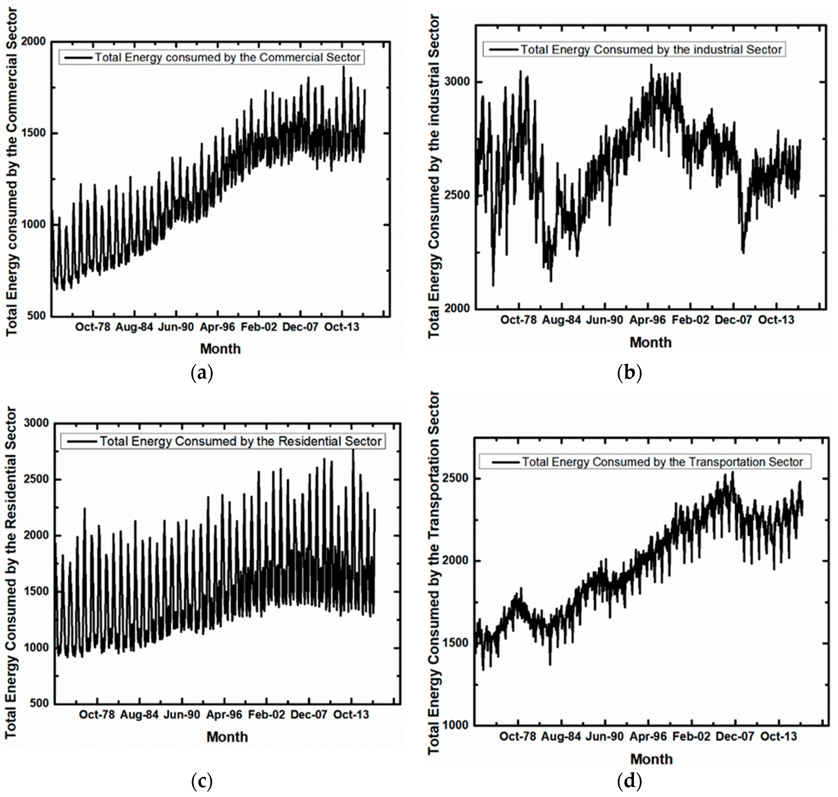
Forecasting energy demand is an important issue for future economic planning because it is required for proper allocation of available resources since energy is linked to industrial production, agricultural output, health, access to water, population, education, and quality of life [11]. Most forecasting methods can be classified into two main methods namely causal and historical data based methods [12]. Causal methods mostly employ energy consumption as the output with some input variables such as economic, social and climate-related factors [12,13,14]. With causal-related methods, artificial neural networks and regression models are the methods frequently used for estimating energy demand. Methods that use historical data leverages past variable-related values to predict energy demand. Most commonly used models under the historical data method are time series, grey prediction and autoregressive models [15]. Forecasting the consumption value of energy demand is important but a challenging task because of energy demand changes according to time horizon, socioeconomic and demographic parameters, as well as climate variables [16]. Complexities in forecasting energy demand may have led core energy modules like the national energy modeling system (NEMS) to develop separate modules for energy demand forecasting. Under this model, characteristics or key features of each sector differs from the other. For example, the Residential Demand Module (RDM) projects energy demand by housing type, census and end-use centering on availability of renewable energy sources, energy prices and changes in housing stock [17], whereas the Commercial Demand Module (CDM) projects energy demand by census division, category of end use and building types hinging on energy prices, availability of renewable sources, equipment availability and fluctuations in commercial floorspace [17]. According to the Energy Information Administration (EIA), RDM and CDM use thirty (30) year historical trends and population projections by integrating variations to heating and cooling degree days by census division. The Industrial Demand Module (IDM) projects energy demand for heat and power in industries as well as feedstock consumption in the chemical industry [17]. Transportation Demand Module (TDM) project energy demand by fuel type focusing on energy process, technological adoption and macroeconomic variables [17]. Due to differences in sectoral characteristics, core energy modules require different energy modeling system for all the sectors [18]. The difference in modeling required for each sector transmits into consumption patterns of each of the sectors. Here, fluctuations in data with respect to our chosen sectors namely: the commercial sector, industrial sector, residential sector and transportation sector are shown in Figure 1a–d respectively. For the United States (U.S.) sectoral energy demand drawn in Figure 1, it is evident that the sectoral differences in respective modules reflect differences in the values as plotted. As each sector has different characteristics and key features, the data replicates what actually goes on in the said sector. For example, the level of consumption for the industrial sector is different from the other respective sectors.
As plotted, it can be deduced that differences in sectoral demand modules and assumptions of high-profile energy modules make sectoral energy demand forecast complex [19]. The complex nature of modeling system transmits into considerably high forecast inaccuracies [20]. Although there may be some considerably high forecast inaccuracies that stem from the NEMS model, NEMS as an energy demand and economic model is able to capture world energy market patterns, resource availability, technological choice and characteristics as well as demographic factors into their model. NEMS design incorporates several modules that interact as part of the equilibrium calculations for long-term patterns. Although the NEMS model is one of the best model replicated by many countries, we propose an assumption-free forecasting algorithm formulation that is also capable of predicting U.S. sectoral energy demand and can be replicated by researchers. We leverage on the power of artificial neural networks (ANNs) in developing an own-data-driven forecasting technique.
Although there are multivariate forecasting techniques like regression models that can be employed herein, we focus on the univariate forecasting technique. The disadvantage of the multivariate forecasting technique is that influential exogenous factors are difficult to determine, and accurate data for them may not be readily available. Nevertheless, univariate forecasting has existed for decades. For example, Saab [21] investigated different univariate-modeling methodologies for monthly electric energy consumption in Lebanon by using the autoregressive, the autoregressive integrated moving average (ARIMA) and a novel configuration combining an AR(1) with a highpass filter. It was concluded that the AR(1)/highpass filter model performed well as against the other techniques. Additionally, Abdel-Aal [15] used both neural and abductive networks to forecast monthly energy demand. In the study, two modeling approaches were investigated and compared: iteratively using a single next-month forecaster, and employing 12 dedicated models to forecast the 12 individual months directly. The results indicated that using a single next-month forecaster is highly accurate. Furthermore, Hu [22] used neural-network-based grey residual modification model to forecast energy demand with authors experimental results verifying that the proposed prediction models performed well. Additionally, Liu [23] forecasted China’s primary energy consumption by comparing multi-variable linear regression (MLR) and support vector regression (SVR) and gated recurrent unit (GRU) artificial neural. The established GRU model resulted in the highest predictive accuracy. As a result of most univariate energy demand projections read, we have seen few papers focusing on sectoral energy demand forecasting. However, we have not seen a paper using Recurrent Neural Network (RNN) based Gated Recurrent Unit (GRU) formulated an algorithm to forecast the energy demand by sector. Motivated by this, we employ the GRU RNNs algorithm that is capable of being utilized for U.S. sectoral energy demand and we test the implementation of our algorithm by applying it to the four sectors chosen. GRU RNNs has achieved success as one of the high-performing ANNs and has been implemented in a number of applications [24,25]. GRU as a nonlinear network flouts the vast assumptions and causal variables needed for future projections and further inculcate dynamism of parameters components like trends, seasonality and smoothing in ensuring the accuracy of future energy demand forecasting [26]. Furthermore, as opposed to a nonlinear network like GRU, linear econometric models require various predictors in predicting energy demand. More specifically, the accuracy of linear models depends on the choice of predictors as there are known and unknown predictors that may influence energy demand [27]. However, data own driven technique like the GRU dismisses the choice of predictors and further accounts for all unknown predictors that may cause volatilities in energy demand [13,23]. Although there are numerous advantages of employing deep learning techniques, most deep learning characteristics of GRU RNNs require massive datasets to help train the system rigorously [26]. With the aim of providing a solution to deep learning techniques requirements for rigorous data, EIA has been reporting monthly data on sectoral consumption over the years. Upon the U.S. being among the top-energy consuming countries in the world with rich massive data on sectoral consumption, the U.S. is also endowed with some of the robust energy-demand forecasting modules. Based on readily available data and its related forecasting modules, we use the U.S. as a case. Monthly data that dates back from January 1973 to December 2016 in Trillion British Thermal Units (TBtu) is employed.
In a nutshell, developing a sequential algorithm based on GRU network will help researchers and stakeholders of the energy market gain insight into future sectoral energy demand consumption levels. Additionally, our GRU algorithm formulation will provide researchers with in-depth information on generating an algorithm required for sectoral energy demand forecasting. As authors have not seen a manuscript using recurrent neural network based gated recurrent unit to forecast sectoral energy demand to the best of our knowledge, this manuscript will help researchers not to use only high-profile energy models as a sole basis of comparison. Rather, researchers can compare their obtained results along with the result of both our formulated algorithm and high-profile energy models. Lastly, this study will help reshape future energy-saving policies and contribute to realizing the climate change targets.
2. Materials and Methods
2.1. Sequential GRU Algorithm Formulation
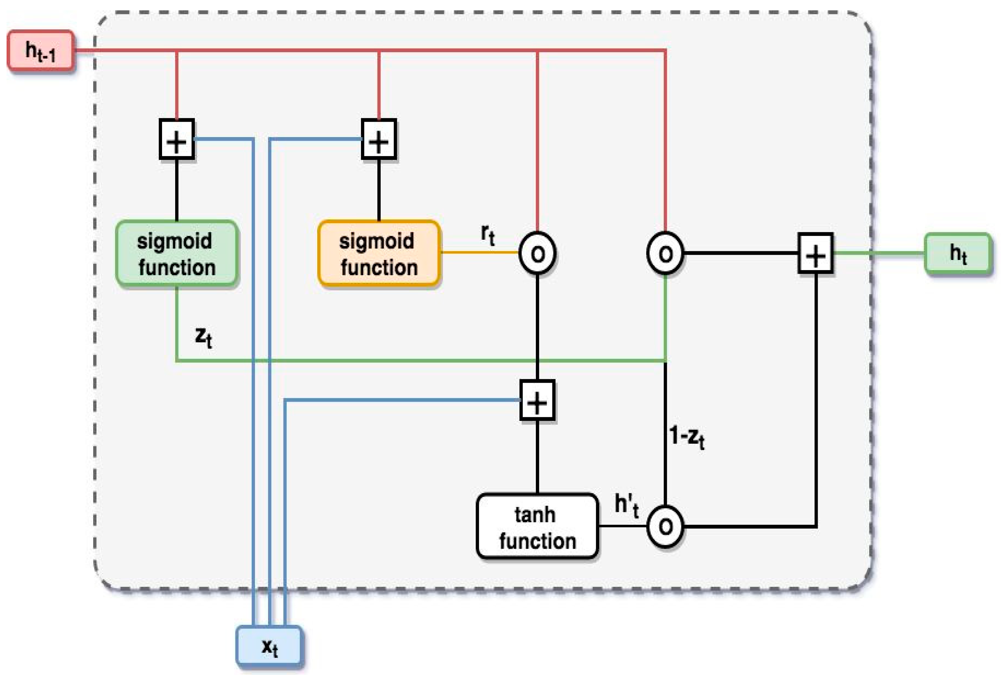
Towards overcoming the inhibitory factors of extant approaches to non-structural forecasting, our sequential algorithm is crafted on the chassis of the GRU network. In a typical analysis of times series data, previous relationships, as time steps increase are difficult to be captured and reflected [28]. Meanwhile, GRU RNNs, which evolved from traditional RNN can consider previous relationships as time progressed [29]. This gives our GRU-based network the ability to information persistence. By virtue of their internal loops, we harness substantial amounts of information that is retained in their architectures as the various sequences of data flow through them. Thus, ensuring good forecast of our consumption parameters. Our detailed version of a single GRU is presented in Figure 2.
GRU, although a variation of RNN focuses on solving the vanishing gradient problem which comes with a standard recurrent neural network through the use of an update gate and a reset gate. The update gate and the reset gate are two vectors that act as a filter, deciding which information should be passed to the output. These two vectors, during training, are made to retain salient information of the past and remove irrelevant information to the prediction. Therefore, we denote our input vector as , represents the output vector, denotes the update gate vector, the reset gate vector, and as the parameter matrices and as the biased vector, represents Hadamard product and represents the sigmoid function. We include a bias vector because it permits the output of our activation to be shifted to the left or right on the x-axis. We start by calculating the update gate vector as
The update gate determines how much past information needs to be passed along to the future. In checking how much information that needs to be excluded from our algorithm, we calculate the out reset gate as
The difference between the update gate and the reset gate stems from the weights and gates used. Finally, we calculate our output vector as
Our sequential algorithm framework initiates with the train and test dataset, which is fed into the architecture as input. Our input module converts the times series dataset to a stationary form, ensuring the ease to dynamically alter the sequence to sequence operations in our network. Like other neural networks, GRUs expect data to be on the scale of the activation function used by the network [30]. We set the activation function for the GRU as a hyperbolic tangent (tanh), which outputs values between −1 and 1, a preferred range for the time series data. Meanwhile, to make the experiment fair, our algorithm scales the coefficient (minimum (min) and maximum (max)) values, calculating them on the training dataset, and applying them to scale the test the dataset and any forecasts. This eludes the experiment with knowledge from the test dataset, which might give our algorithm a small edge. The MinMax Scaler module transforms the dataset to the range [−1, 1], thus performing a normalization on the inputs. Mathematically, we formulate this as
where - original value, - normalized value.
With this setup, the model prevents ill-conditioning. In essence, guaranteeing the stable convergence of weight and biases.
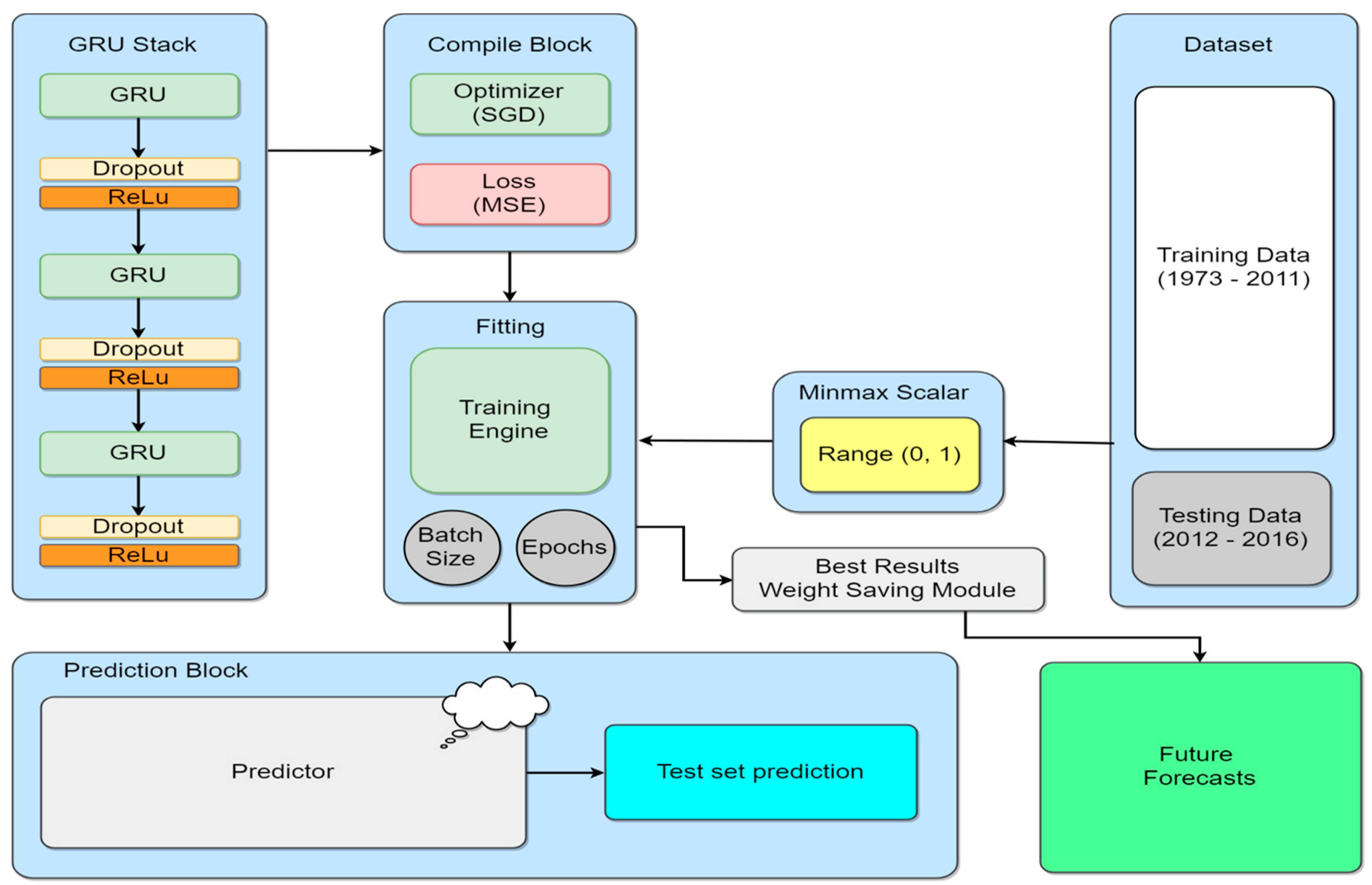
To enhance forecast accuracies and its subtle behaviors covered by the trends volatility, our algorithm again utilizes a stack of GRUs. Stacking our GRUs hidden layers makes our algorithm deeper, accurately earning the description as a deep learning technique [31]. Each layer processes some part of the task we wish to solve and passes it on to the next until finally, the last layer provides the output. Increasing the depth of our network provides an alternate solution, requiring fewer neurons and training faster. Ultimately, our algorithm achieves a representational optimization.
We set Rectified linear units (ReLu) as our algorithm’s activation function [32]. Activation functions are an extremely important feature of the artificial neural networks. The activation function is the non-linear transformation that we do over our algorithm’s input signal in the GRU stack. This transformed output is then sent to the next layer of neurons as the input among the GRUs. They basically decide whether a neuron should be activated or not. That is, whether the information that the neuron is receiving is relevant for the given information or should it be ignored.
We also included Dropout blocks in our algorithm [33]. The Dropout block aided in randomly selecting neurons, which are thereafter ignored during training. These dropouts ensured that some neurons’ contribution to the activation of downstream neurons is temporally removed on the forward pass and any weight updates are not applied to the neuron on the backward pass. As our algorithm’s neural network learns, neuron weights settle into their context within the network. Weights of neurons are tuned for specific features providing some specialization. Neighboring neurons rely on this specialization, which, if taken too far, can result in a fragile model too specialized for the training data. Hence, we make our algorithm withstand complex co-adaptations. The effect is that our algorithm’s neural network becomes less sensitive to the specific weights of neurons. This results from our algorithm’s capabilities of better generalizing the forecasting task, and less likely to overfit the training data.
During the compilation of our algorithm, we employed Adam Optimizer as our optimizer [34]. We preferably use Adam Optimizer because it is different to classical stochastic gradient descent. Stochastic gradient descent usually maintains a single learning rate for all of its weight updates with a zero change in learning rates during training. Adams Optimizer maintains a learning rate for each networks weight which is separately updated as learning unfolds. Again, we use Adam because it realizes the benefit of both Adaptive Gradient Algorithm (AdaGrad) and Root Mean Square Propagation (RMSProp). Adam goes a step further to use the average of the second moments of the gradients (the uncentered variance) instead of adapting parameter learning rates based on the average first moment (the mean). We also use the mean squared error as our loss function. The loss function is an important part of artificial neural networks, which is used to measure the inconsistency between predicted values and actual labels during the training time. It is a non-negative value, where the robustness of model increases along with the decrease of the value of loss function. Our algorithm then fits the whole setup for predictions. The fitting module trains the algorithm for a fixed number of epochs on the data.
We tune our algorithm’s parameters on the basis of batch-size, number of epochs, different optimizers and the number of hidden layers of the GRU stack. We used a batch size of 4 and kept the window size at 12 as this gave us the most optimized output. We also use a stack of 10 layers and the number of iterations needed to obtain the optimized results is 300. Our best performing weight is then saved, of which we use for our forecast. Our main algorithm formulation is presented in Figure 3.
2.2. Error Indexes
In estimating the performance of an algorithm, we used the year-over-year errors (YoY), mean absolute deviation (MAD), mean absolute percentage error (MAPE) and root mean square error (RMSE) as used by reference [35]. Denoting the realized values in a particular year as and as our forecasted values in a particular year, the YoY errors is expressed as
The expression whose absolute value is computed at the numerator of Equation (5) signals the presence of an undercast if or of an overcast if . We then calculate the overall indexes (MAD, MAPE, and RMSE) as
where is the realized value, is the forecasted value, is the number of periods forecasted and is the YoY error.
3. Results
Here, sectoral (commercial sector, industrial sector, residential and transportation) monthly data extracted from the Monthly Energy Review published by the U.S. Energy Information Administration (EIA) is used in our study. The initial data TBtu is converted to science index unit exajoules (EJ) using International the Energy Administration (IEA) unit converter; where 1 TBtu = 0.00105505585 EJ [36]. In checking the forecast accuracy and error of the GRU, monthly data for the four sectors spanning from January 1973 to December 2011 is used as a training set whereas monthly data from January 2012 to December 2016 is used as a test set. We then convert the predicted monthly test set values for each of the sectors to yearly values. We compare the output from GRU and our benchmark AEO2008 [37] yearly forecast as against the realized values for the defined yearly test set data. Finally, the yearly projections from the GRU and AEO2018 [38] projections to 2021 are presented in EJ. AEO2018 initial forecast in Quadrillion British thermal units (QBtu) is converted to EJ using the IEA unit converter; where 1 QBtu = 1.05505585 EJ [36].
3.1. Comparison and Forecasting of Total Energy Consumption by the Commercial Sector
3.1.1. Commercial Sector Comparison of GRU and AEO2008 Benchmark Results as Against Realized Values
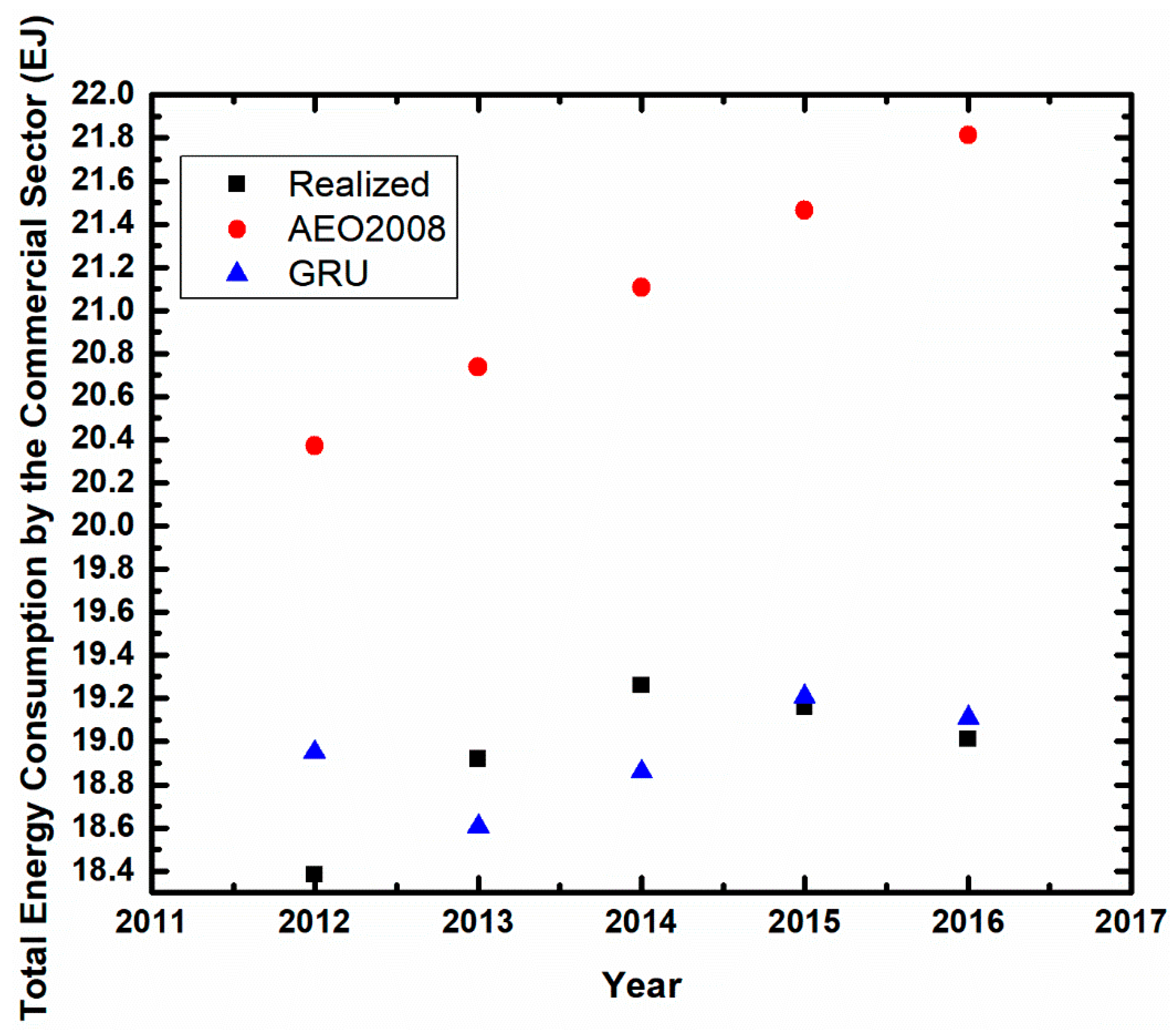
Realized values for total energy consumption by the commercial sector covering the period of 2012 to 2016 is ~18.38085 EJ; ~18.91966 EJ; ~19.25928 EJ; ~19.15798 EJ; and ~19.00906 EJ respectively (see Table 1 and Figure 4). Comparing AEO2008 as against realized values, AEO2008 forecast reports ~20.37100 EJ (overcast of ~10.38%) in 2012; ~20.73709 EJ (overcast of ~9.61%) in 2013; ~21.10715 EJ (overcast of ~9.60%) in 2014; ~21.46399 EJ (overcast of ~12.04%) in 2015; and ~21.81230 EJ (overcast of ~14.75%) in 2016 (see Table 1 and Figure 4). ANN-based GRU reports ~18.94859 EJ for 2012 indicating an overcast of ~3.09%; ~18.60560 EJ for 2013 representing an undercast of ~1.67%; ~18.85887 EJ for 2014 representing an undercast of ~2.08%; ~19.20703 EJ for 2015 indicating an overcast of ~0.26%; and ~19.10947 EJ for 2016 depicting an overcast of ~0.84% (see Table 1 and Figure 4). Comparing both the GRU and AEO2008 forecast as against the realized values, our technique reports an improvement of ~4-fold for 2012; ~6-fold for 2013; ~5-fold for 2014; ~46-fold for 2015 and ~28-fold for 2016 (see Table 1). AEO2008′s MAD, MAPE, and RMSE is ~2.15294, ~11.36234, and ~2.18422 respectively (see Table 1). GRU’s MAD, MAPE, and RMSE is ~0.28633, ~1.52241, and ~0.34461 (see Table 1). Using the MAPE index as our benchmark, our technique presents an improvement of ~8-fold (see Table 1). Here, we conclude that our ANN based GRU enormously outperforms the EO2008 forecast for the total energy consumption by the commercial sector.
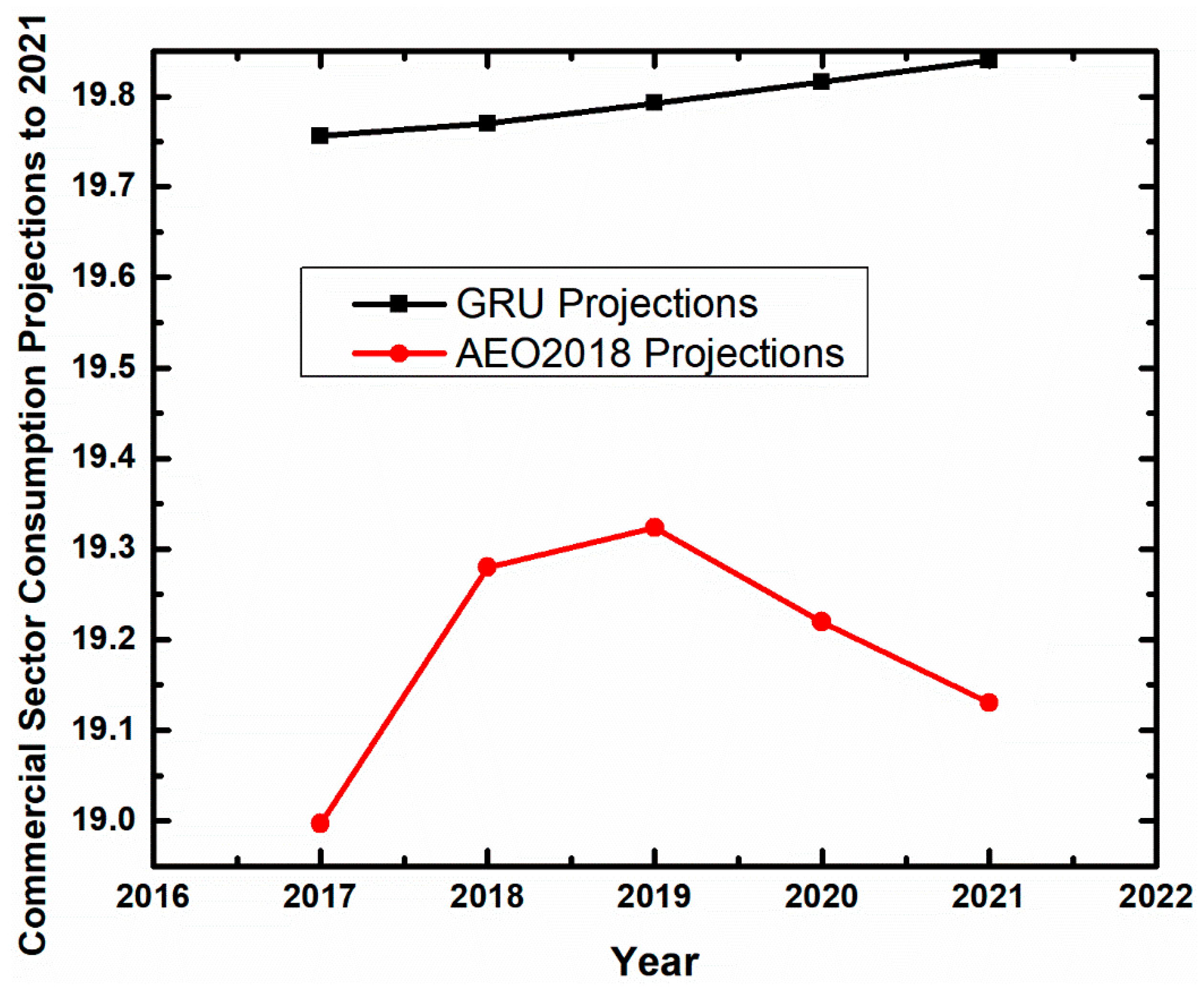
3.1.2. Forecasting Total Energy Consumption by the Commercial Sector to the Year 2021
Commercial sector total energy consumption by the GRU and AEO2018 in EJ is represented in Figure 5. GRU projections for commercial sector depicts that yearly consumption for the period covering 2017 to 2021 will be ~19.75606671 EJ; ~19.77006140 EJ; ~19.79258424 EJ; ~19.81555476 EJ; and ~19.83966134 EJ respectively. Meanwhile, AEO2018 projections covering the same time period is ~18.99668994 EJ for 2017; ~19.28014547 EJ for 2018; ~19.3239345 EJ for 2019; ~19.21951668 EJ for 2020; and ~19.12976519 EJ for 2021. GRU and AEO2018 projection for the year 2021 suggest ~4.2% and 0.6% increase from 2016 total commercial sector consumption level (~19.0090605 EJ).
3.2. Comparison and Forecasting of Total Energy Consumption by the Industrial Sector
3.2.1. Industrial Sector Comparison of GRU and AEO2008 Benchmark Results as against Realized Values
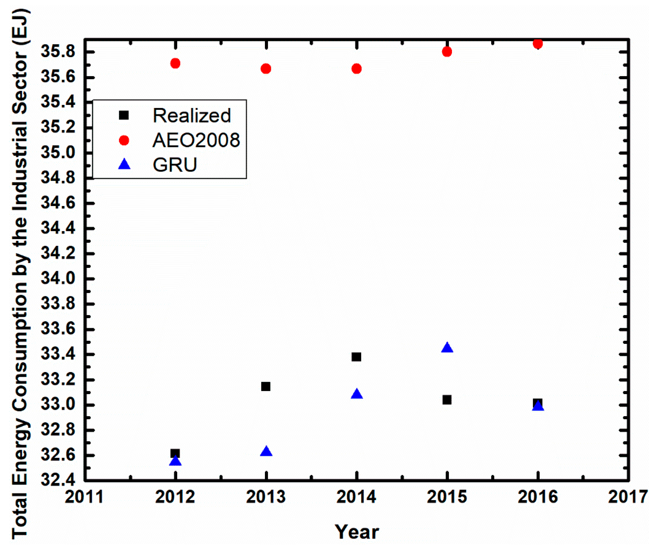
Realized values for total energy consumption by the industrial sector covering the period of the years 2012 to 2016 is ~32.61324 EJ; ~33.14342 EJ; ~33.38001 EJ; ~33.03884 EJ; and ~33.01164 EJ respectively (see Table 2 and Figure 6). Comparing with the realized values, AEO2008 forecast reports ~35.70989 EJ for 2012 (an overcast of ~9.50%); ~35.66654 EJ for 2013 (an overcast of ~7.61%); ~35.66670 EJ for 2014 (an overcast of ~6.85%); ~35.80256 EJ for 2015 (an overcast of ~8.37%); and ~35.8678 EJ for 2016 (an overcast of ~8.65%) (see Table 2 and Figure 6). GRU presents ~32.54658 EJ for 2012 (an undercast of ~0.20%); ~32.62127 EJ for 2013 (an undercast of ~1.56%); ~33.07801 EJ for 2014 (an undercast of ~0.90%); ~33.44679 EJ for 2015 (an overcast of ~1.23%); and ~32.98164 EJ for 2016 (an undercast of ~0.09%) (see Table 2 and Figure 6). GRU presents an improvement of ~48-fold; ~5-fold; ~8-fold; ~7-fold; and ~10-fold, respectively (see Table 2). AEO2008 MAD is ~2.70529; MAPE is ~8.19511; and RMSE is ~2.71958 (see Table 2). GRU MAD is ~0.26575; MAPE is ~0.80204; and RMSE is ~0.32730 (see Table 2). Using the MAPE index as our benchmark, our technique presents an improvement of ~10-fold (see Table 2). Again, the GRU has outperformed the AEO2008 predictions for the total energy consumption by the industrial sector.
3.2.2. Forecasting Total Energy Consumption by the Industrial Sector to the Year 2021
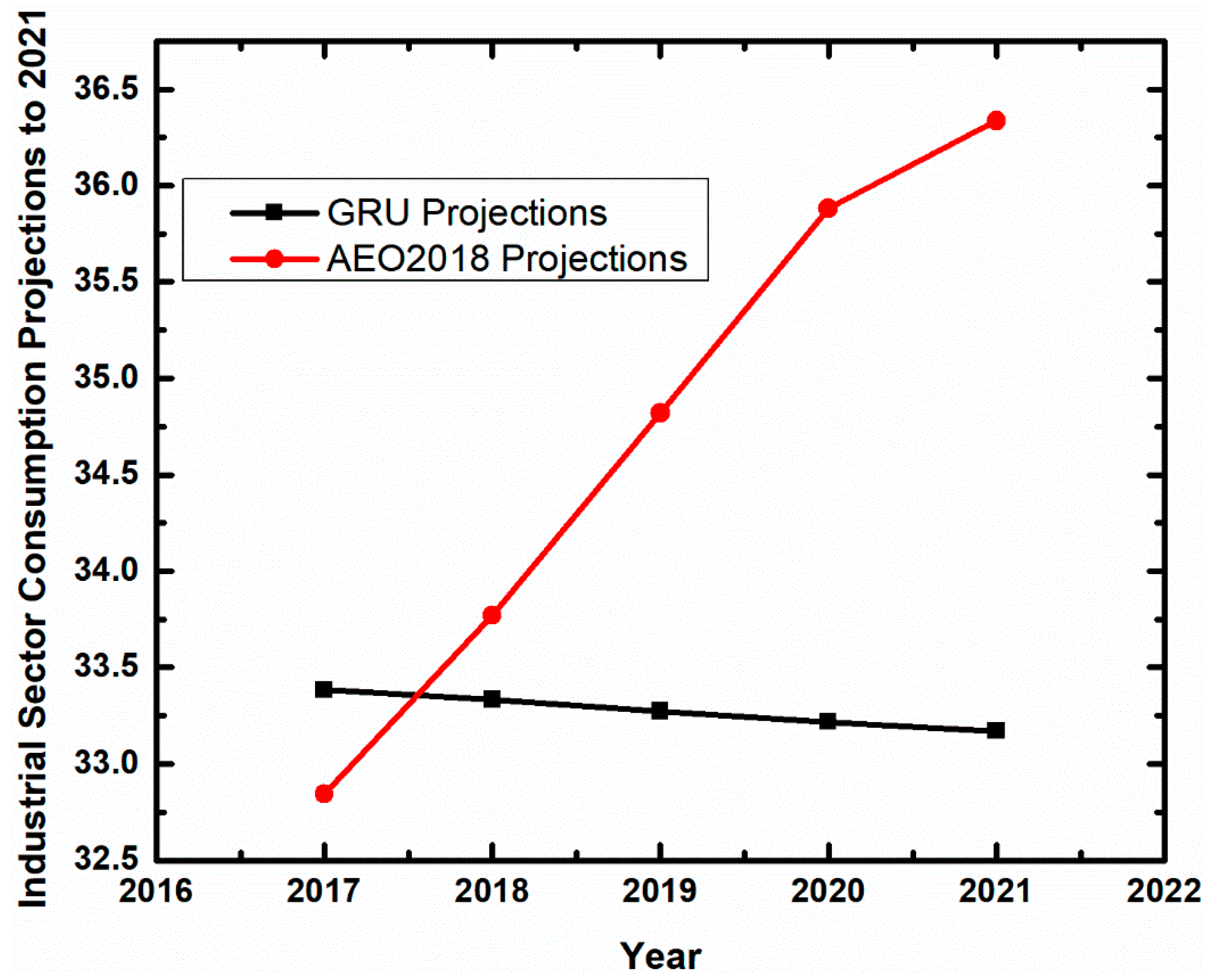
Figure 7 represents GRU and AEO2018 yearly projections of total energy consumption by the industrial sector in EJ. GRU projections show ~33.38505756 EJ for 2017; ~33.33334257 EJ for 2018; ~33.2728023 EJ for 2019; ~33.21667776 EJ for 2020; and ~33.17049743 EJ for 2021. AEO2018 projections reports ~32.84340856 EJ; ~33.76928548 EJ; ~34.81909243 EJ; ~35.88140495 EJ; and ~36.33706775 EJ for 2017, 2018, 2019, 2020 and 2021 respectively. GRU and AEO propose an increase from the 2016 total industrial sector consumption level (33.01163616 EJ) by ~0.48% and 10.07% respectively.
3.3. Comparison and Forecasting of Total Energy Consumption by the Residential Sector
3.3.1. Residential Sector Comparison of GRU and AEO2008 Benchmark Results as Against Realized Values
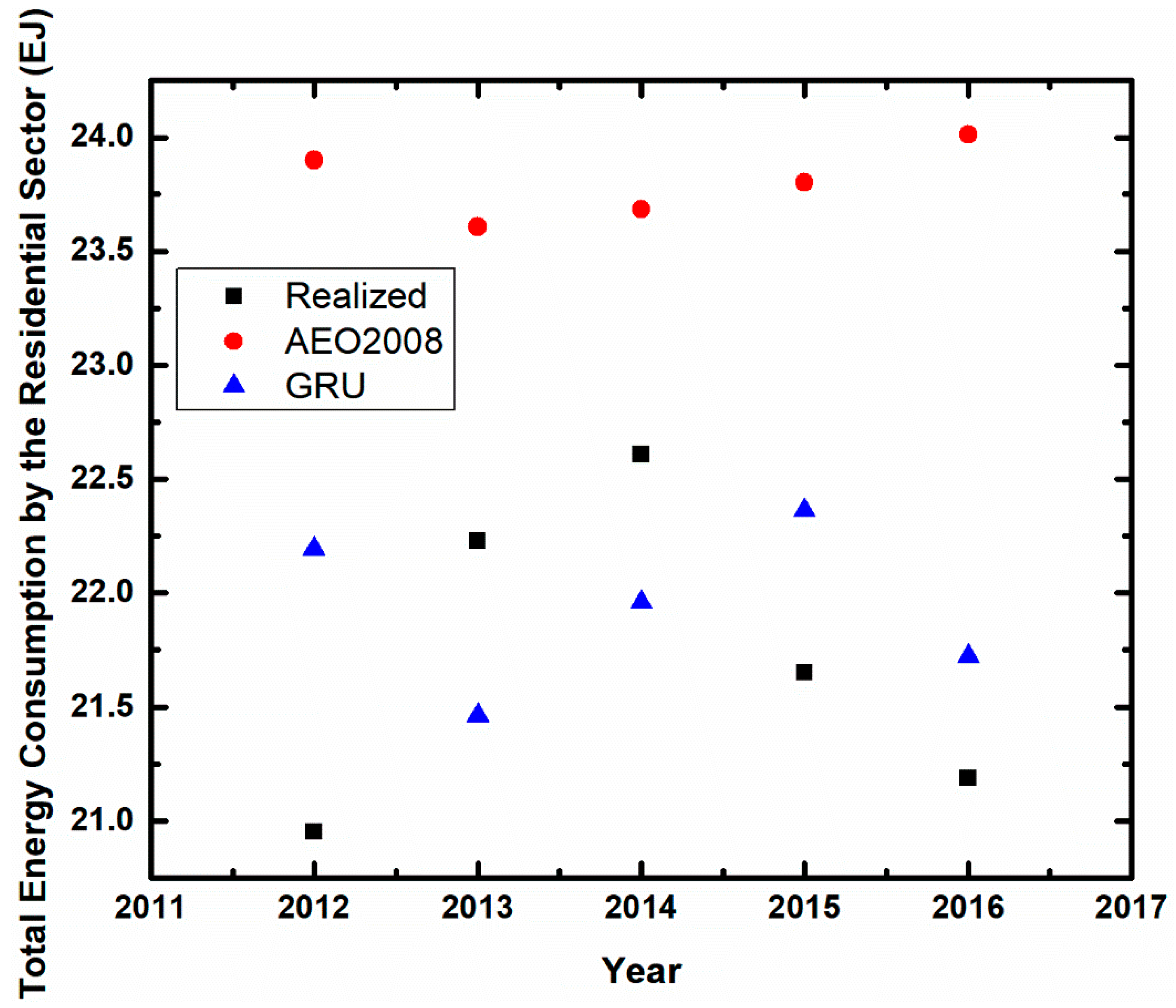
Realized values for total energy consumption by the residential sector is ~20.95077 EJ for 2012; ~22.22864 EJ for 2013; ~22.60793 EJ for 2014; ~21.64991 EJ for 2015; and ~21.18855 EJ for 2016 (see Table 3 and Figure 8). AEO2008 reports ~23.90059 EJ (an overcast of ~14.08%); ~23.60672 EJ (an overcast of ~6.20%); ~23.68307 EJ (an overcast of ~4.76%); ~23.80177 EJ (an overcast of ~9.94%); and ~24.01367 EJ (an overcast of ~13.33%) (see Table 3 and Figure 8). Meanwhile, GRU reports ~22.19425 EJ for 2012 (an overcast of ~5.93%); ~21.46197 EJ for 2013 (an undercast of ~3.44%); ~21.95929 EJ for 2014 (an overcast of ~2.87%); ~22.36165 EJ for 2015 (an overcast of ~3.29%); and ~21.72201 for 2016 (an undercast of ~2.52%) (see Table 3 and Figure 8). GRU presents an improvement of ~2-fold for 2012; ~2-fold for 2013; ~2-fold for 2014; ~3-fold for 2015; and ~5-fold for 2016 (see Table 3). MAD, MAPE and RMSE for AEO2008 is ~2.07600; ~9.66149; and ~2.20763 respectively (see Table 3). Similarly, MAD, MAPE, and RMSE for GRU are 0.78079, ~3.61169, and ~0.81804 respectively (see Table 3). Likewise, using the MAPE as our benchmark index, our technique presents an improvement of ~3-fold (see Table 3). Again, we conclude that the GRU has outperformed the AEO2008 predictions for the total energy consumption by the residential sector.
3.3.2. Forecasting Total Energy Consumption by Residential Sector to the Year 2021
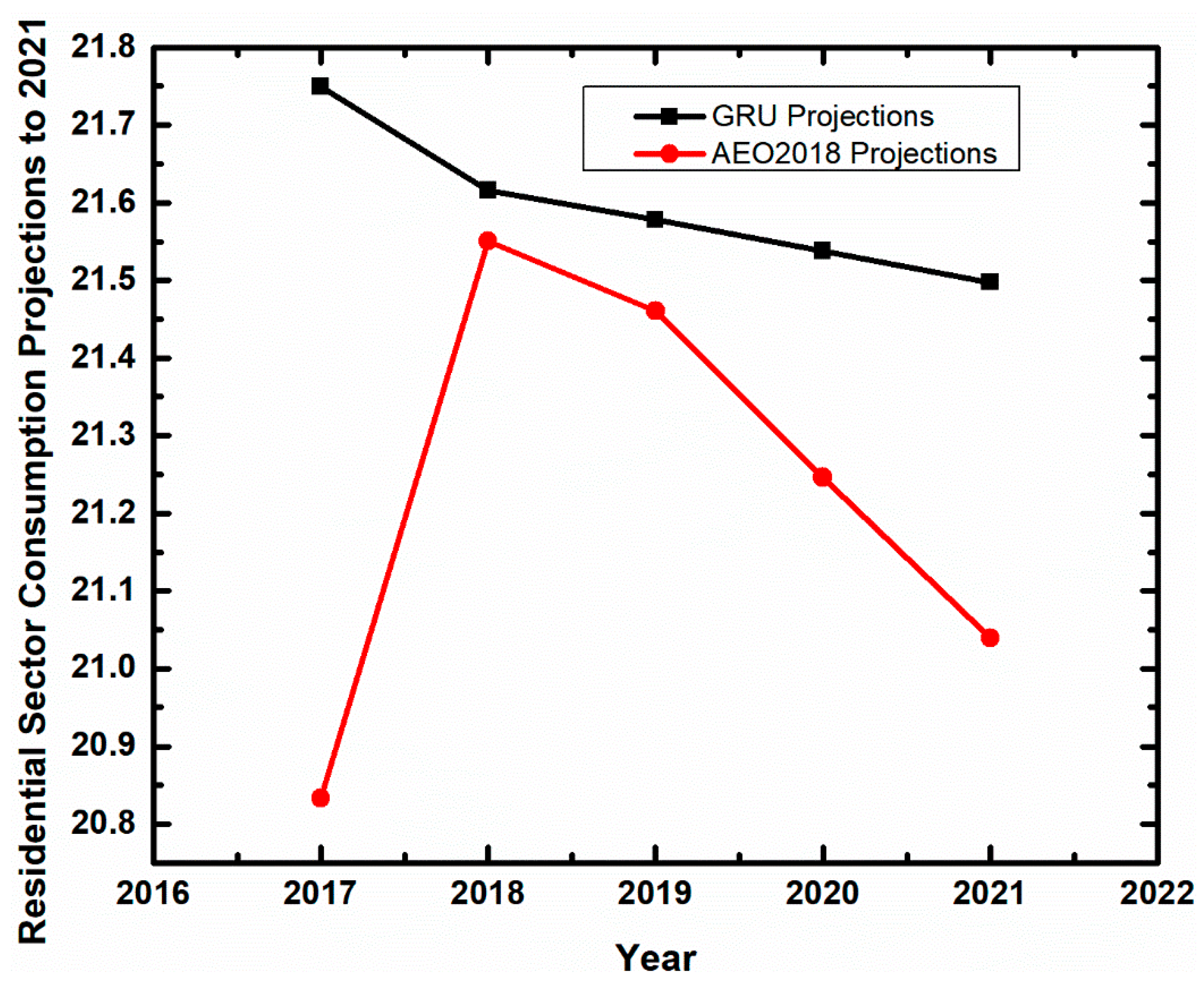
Figure 9 shows the GRU and AEO2018 residential sector yearly projections in EJ to the year 2021. GRU forecast total energy consumption by the residential to be ~21.74933832 EJ in 2017; ~21.61585907 EJ in 2018; ~21.5776916 EJ in 2019; ~21.53756071 EJ in 2020; and ~21.49758875 EJ in 2021. AEO2018 projections reports ~20.83338497 EJ for 2017; ~21.55023528 EJ for 2018; ~21.46090265 EJ for 2019; ~21.24635493 EJ for 2020; and ~21.03896683 EJ for 2021. GRU estimates an increase in the 2016 residential sector consumption level (~21.18855159 EJ) by ~1.46% whereas AEO2018 suggests a decrease in 2016 residential sector consumption level (~21.18855159 EJ) by ~0.71%.
3.4. Comparison and Forecasting of Total Energy Consumption by the Transportation Sector
3.4.1. Transportation Sector Comparison of GRU and AEO2008 Benchmark Results as Against Realized Values
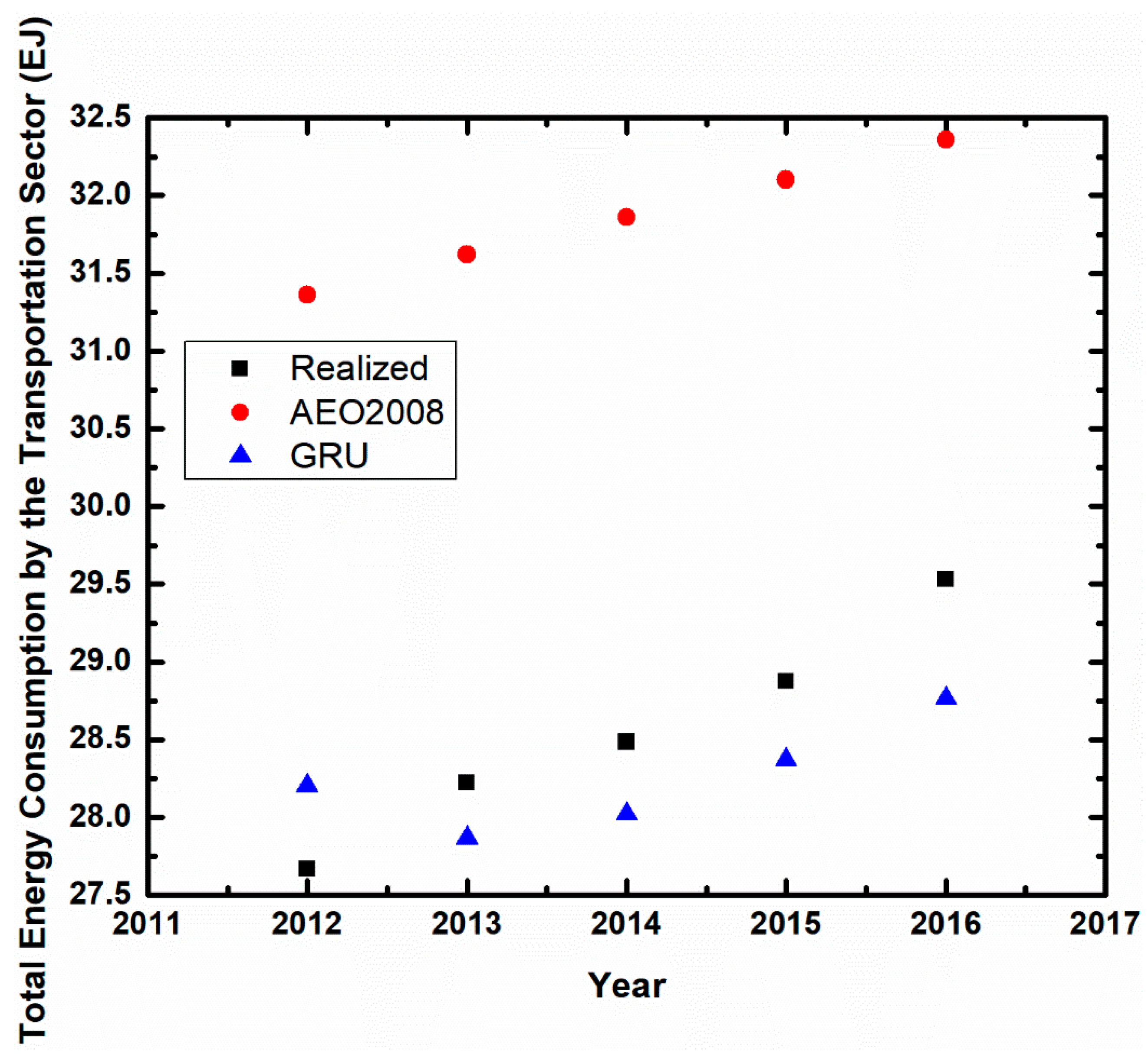
Realized values for total energy consumption by the transportation sector for the period covering 2012 to 2016 is ~27.66272 EJ; ~28.22262 EJ; ~28.48267 EJ; ~28.87517 EJ; and ~29.53091 EJ respectively (see Table 4 and Figure 10). AEO2008 projections for the transportation sector is ~31.36073 EJ for 2012 (an overcast of ~13.37%); ~31.61988 EJ for 2013 (an overcast of ~12.04%); ~31.86202 EJ for 2014 (an overcast of ~11.86%); ~32.09991 EJ for 2015 (an overcast of ~11.17%); and ~32.35749 EJ for 2016 (an overcast of ~9.5%) (see Table 4 and Figure 10). GRU presents ~28.20137 EJ for 2012 (an overcast of ~1.95%); ~27.86641 EJ for 2013 (an undercast of ~1.26%); ~28.02113 EJ for 2014 (an undercast of ~1.46%); ~28.37007 EJ for 2015 (an undercast of ~1.75%); and ~28.76440 EJ for 2016 (an undercast of ~2.60%) (see Table 4 and Figure 10). On the YoY basis, GRU records an improvement of ~7-fold for 2012; ~10-fold for 2013; ~7-fold for 2014; ~6-fold for 2015; and ~4-fold for 2016 (see Table 4). MAD, MAPE, and RMSE for AEO2008 is ~3.30519, ~11.60192, and ~3.31738. MAD, MAPE, and RMSE for GRU is ~0.52561, ~1.83495, and ~0.54272 (see Table 4). Using MAPE as our benchmark index, our technique presents an improvement of ~6-fold (see Table 4). Again, our technique presents an enormous improvement on the AEO2008 predictions for the total energy consumption by the transportation sector.
3.4.2. Forecasting Total Energy Consumption by Transportation Sector to the Year 2021
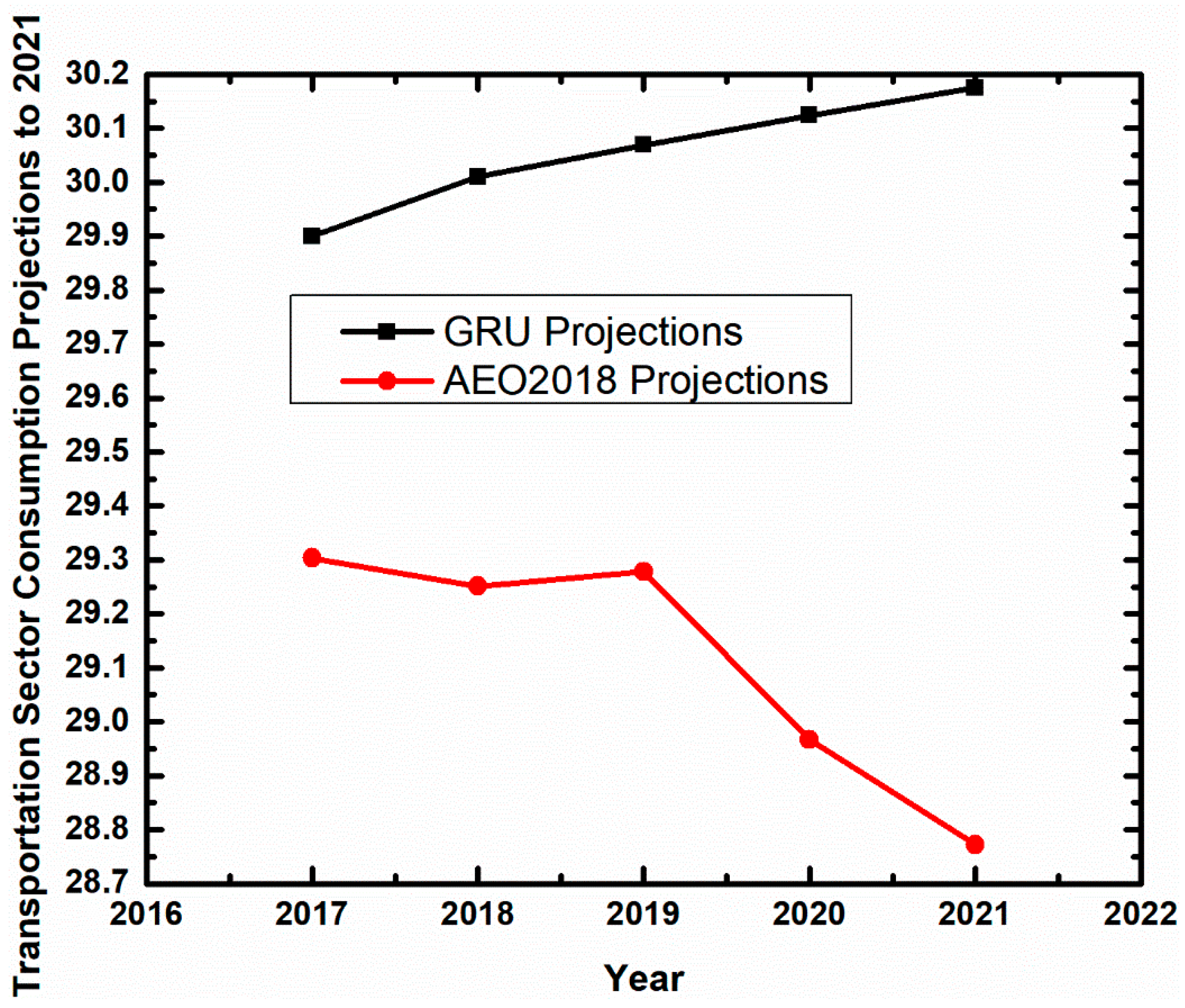
Figure 11 depicts the GRU and AEO2018 transportation sector total energy consumption yearly projections in EJ to 2021. GRU reports ~29.89975191 EJ for 2017; ~30.00996867 EJ for 2018; ~30.06909301 EJ for 2019; ~30.12371611 EJ for 2020; and ~30.17492083 EJ for 2021. AEO2018 projections suggest that total energy consumption from the transportation sector will be ~29.30341132 EJ in 2017; ~29.25143610 EJ in 2018; ~29.27883063 EJ in 2019; ~28.96598441 EJ in 2020; and ~28.77181404 EJ in 2021. Using the 2016 total transportation sector consumption level (29.53091301 EJ) as a benchmark, GRU suggest an increase of ~2.18% by the 2016 level whereas AEO2018 estimates a decrease in the 2016 total consumption level by ~2.63%.
4. Discussion
As the world evolves, countries are enacting policy measures to ensure effective utilization of energy-related resources. Benefits derived from energy efficiency levels to a country are manifold. Accurate efficiency measures correspond to improved air quality, greenhouse gas emissions reduction; sustainable energy bills and security, as well as deferred infrastructure cost [39,40]. Government policies on energy efficiency correspond to the interplay of federal, state, and local jurisdictional levels. However, measuring policy impacts have taken a toll on various policymakers [41]. Without accurate and reliable methods, implementation of policies based on unreliable measures and procedures exerts colossal costs on government generated revenues. As stated earlier, projections from assumption-driven core modules are likely not to accurately model intricate patterns in a dataset, thereby transmitting into considerably high forecast errors. At a particular year, high overcast or undercast of demand implies that countries may waste expenditure on consumption levels which can be invested in other sectors of an economy.
Few research aricles has considered sectoral energy demand forecasting. For example, in forecasting long-term electricity demand for the residential sector, Pessanha [42] decomposed the total electricity residential consumption into three components, namely: average consumption per consumer unit, electrification rate, and the number of households and forecasted total electricity consumption in the residential sector by finding the product of the three components. The proposed methodology provided a framework to integrate the macroeconomic scenario, demographic projection, and assumptions for ownership and efficiency of electric appliances in a ten (10) year demand forecast for Brazil. Additionally, Kialashaki [43] investigated the energy demand of each sector separately using the analysis of trend for a unique set of independent parameters which affect the energy demand in that sector using artificial neural network by choosing independent variables that provide the most precise estimate of the dependent variable. For the residential sector, it was concluded by Reference [43] that multiple linear regression and artificial neural network models depict a similar level of accuracy for the testing stage; artificial neural networks outperformed multiple linear regression for the transportation sector; the artificial neural network was used to forecast the industrial energy demand by concluding that the ascending price scenario and descending price scenario will result in a 7% and 25% increase in the energy demand of this sector, respectively; for the commercial sector forecast, it was concluded that the ascending trade scenario and descending trade scenario will result in a 5% and 2% increase in the energy demand of this sector, respectively. For all the papers we have come across cited herein, it will be ideal if we compare our results with those papers based on a similar timespan and approach. Yet, as these research papers leveraged the inherent interaction of the causal variables, our approach is free of causal variables. Therefore, our step by step specified algorithm formulation that hinges on the recurrent neural network based gated recurrent unit can be implemented and improved upon. By so doing, there will be volumes of forecasting projections based on a gated recurrent unit for the sectoral energy demand for comparison.
With substantial evidence from our testing stage that our GRU network projected results outperformed AEO2008 projections, the initial claim that researchers replicating our algorithm formulation or formulating a new deep learning GRU algorithm can compare their projected results with our obtained results together with the results from top-energy model projections is achieved. Our step by step mathematical algorithm formulation aims to help researchers and energy stakeholders mimic our algorithm formulation for an improve forecasting. By so doing, researchers will provide in-depth information to stakeholders and policymakers on future consumption levels to aid their investment plans as well as implementing sustainable future export and import policies for the ultimate goal of sustainability.
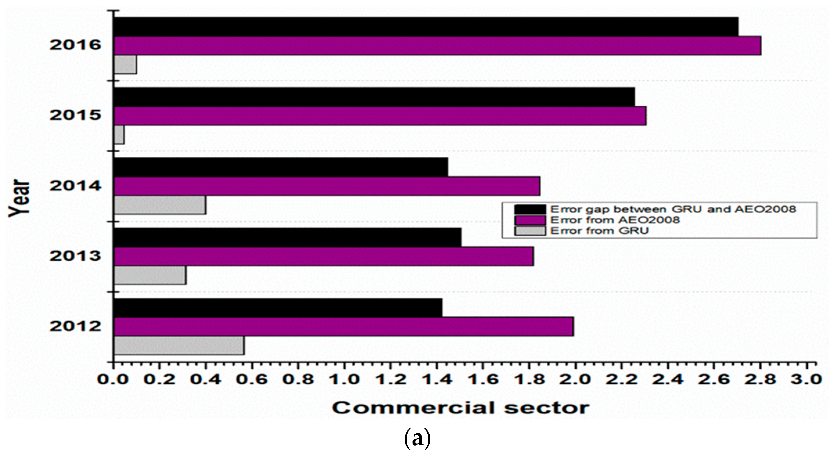
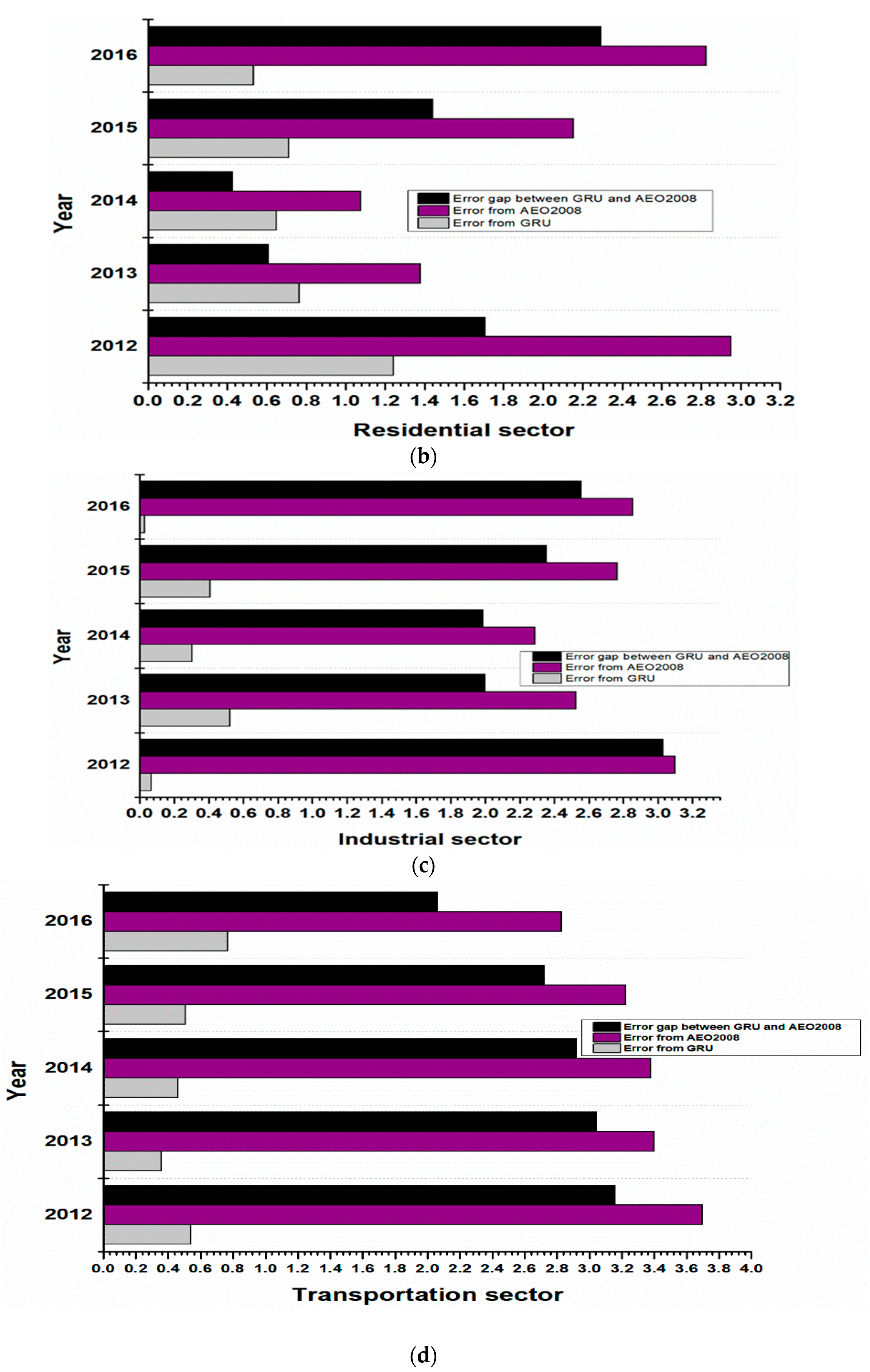
With the aim of providing readers with an accurate insight on the performance of our GRU algorithm projections and AEO2008 projections, we make an error analysis to depict how the two approaches deviate from each other as well as how the two approaches deviate from the realized values. Here, we make a consumption error analysis for our test datasets covering the period of 2012 to 2016 for all the sectors herein. We analyze how spread AEO2008 and our GRU is from realized values. In calculating the error for both AEO2008 and GRU, we take the absolute value of the difference between AEO2008 and the realized values as well as the absolute value of the difference between GRU and the realized values. The absolute value of the difference between AEO2008 and the realized values is the error from AEO2008 projections whereas the absolute value of the difference between GRU projections and the realized values is referred to as the error from our GRU technique. We then find the difference in errors obtained for both the AEO2008 and GRU technique with the aim of finding the gap in errors in each year of our testing stage. The consumption error gap between our GRU network projections and AEO2008 projections for the commercial is ~1.42241 EJ in 2012, ~1.50337 EJ in 2013, ~1.44746 EJ in 2014, ~2.25696 EJ in 2015, and ~2.70283 EJ in 2016 (see Figure 12a). Likewise, the consumption error gap for the industrial is ~3.02999 EJ in 2012, ~2.00097 EJ in 2013, ~1.98469 EJ in 2014, ~2.35577 EJ in 2015, and ~2.55623 EJ in 2016 (see Figure 12b). Similarly, the consumption error gaps for the residential sector are ~1.70634 EJ, ~0.61141 EJ, ~0.4265 EJ, ~1.44012 EJ, and ~2.29166 EJ for the periods of 2012, 2013, 2014, 2015, and 2016, respectively (see Figure 12c). Finally, the consumption error gap for the transportation sector is ~3.15936 EJ in 2012, ~3.04105 EJ in 2013, ~2.91781 EJ in 2014, ~2.71964 EJ in 2015, and ~2.06007EJ in 2016 (see Figure 12d).
5. Conclusions
Forecasting energy consumption is a prerequisite to information on future consumption levels and gives insight into implementing effective and efficient policy tools. Policymakers generally rely on high accuracy forecasts in designing energy realistic energy policies [35]. However, the existing energy demand forecasting models require numerous endogenous and exogenous causal variables as well as assumptions in forecasting, which have spilled-over high forecasting inaccuracies in previous AEO projections. In ensuring the predictive accuracy of a future forecast from linear models, the effects of causal variables (GDP, population, prices of energy demand by sector, inflation, and income) used in previous AEO projections must be assumed. The assumptions required from all the causal variables renders AEO past projections to deviate from the realized values.
We contribute to the literature by presenting an assumption-free-based high accuracy GRU algorithm for medium-term forecasting of sectoral energy demand. Our GRU algorithm processing of time series data is considered superior because the MAPE error of our predicted results is low. Our GRU algorithm could present itself as one of the best techniques in deep learning because our monthly data obtained has been used to predict yearly sectoral energy demand by using our GRU-based formulated algorithm on our test data. Subsequently, our algorithm has been used to forecast the yearly sectoral energy demand until 2021. Our zero assumption based sequential algorithm devoid of causal variables can be replicated by researchers by following the steps and mathematical formulation provided in our sequential algorithm formulation. Although there are more predictive testing tools and methods that can be implemented, our algorithm formulation and projections can provide policymakers with estimated future consumption levels in order to enact realistic and reliable energy policies for implementation.
Our estimated projections showing that consumptions for the commercial sector, industrial sector, residential sector, and transportation in 2021 will be ~19.83966134 EJ, ~33.17049743 EJ, ~21.49758875 EJ, and ~30.17492083 EJ, respectively, and are likely to inform government decision makers and sectoral energy demand stakeholders about future consumption levels. Thus, the prediction of sectoral energy demand will help to plan future investments, access volumes of investments required, as well as manage energy import and export policies.
In the nutshell, this study concludes that our medium-term forecast output presented a significant improvement in the existing high-profile NEMS model.
6. Limitations of Our GRU Algorithm
To make our algorithm learn well, a more robust GRU network is required. Although our algorithm utilized monthly data, a substantial amount of data such as weekly or daily data can accurately mimic the intricate patterns in our datasets compared to the monthly datasets. Additionally, the inclusion of proposed sectoral energy demand policies in our algorithm formulation will help shift the training of the data for an improve forecast projections. Thus, in our future research work on sectoral demand forecasting, we would include sectoral energy demand policies for a more accurate and improved forecasting.
Author Contributions
B.A. and L.Y. conceived and designed the study; B.A. and L.Y. wrote the first draft; B.A. analyzed the data; B.A. and L.Y. wrote and edited the final manuscript for publication.
Funding
This research was funded by the China Scholarship Council monthly stipend given to the leading author.
Acknowledgments
I would like to thank Li Yao and Ma Yongkai for offering their expert advice throughout the manuscript.
Conflicts of Interest
The authors declare no conflict of interest.
References
- Timmons, D.; Harris, J.M.; Roach, B. The Economics of Renewable Energy. Renew. Energy 2009, 1341–1356. [Google Scholar] [CrossRef]
- Oyedepo, S.O. Energy and sustainable development in Nigeria: The way forward. Energy Sustain. Soc. 2012, 2. [Google Scholar] [CrossRef]
- Fu, K.S.; Allen, M.R.; Archibald, R.K. Evaluating the relationship between the population trends, prices, heat waves, and the demands of energy consumption in cities. Sustainability 2015, 7. [Google Scholar] [CrossRef]
- Payne, J.E. On the Dynamics of Energy Consumption and Employment in Illinois. J. Reg. Anal. Policy 2009, 39, 126–130. [Google Scholar]
- Sadorsky, P. Renewable energy consumption and income in emerging economies. Energy Policy 2009. [Google Scholar] [CrossRef]
- Mohiuddin, O.; Asumadu-sarkodie, S.; Obaidullah, M. The relationship between carbon dioxide emissions, energy consumption, and GDP: A recent evidence from Pakistan energy consumption, and GDP: A recent evidence. Cogent Eng. 2016, 1, 1–16. [Google Scholar] [CrossRef]
- Saidi, K.; Hammami, S. The impact of CO2 emissions and economic growth on energy consumption in 58 countries. Energy Rep. 2015, 1, 62–70. [Google Scholar] [CrossRef]
- Strbac, G. Demand side management: Benefits and challenges. Energy Policy 2008, 36, 4419–4426. [Google Scholar] [CrossRef]
- Zou, C.; Zhao, Q.; Zhang, G.; Xiong, B. Energy revolution: From a fossil energy era to a new energy era. Nat. Gas Ind. B 2016, 3, 1–11. [Google Scholar] [CrossRef]
- Wen, Y. The Making of an Economic Superpower-Unlocking China’s Secret of Rapid Industrialization; World Scientific: Singapore, 2015; pp. 1–180. [Google Scholar]
- Suganthi, L.; Samuel, A.A. Energy models for demand forecasting—A review. Renew. Sustain. Energy Rev. 2012, 16, 1223–1240. [Google Scholar] [CrossRef]
- Singh, A.K.; Khatoon, S. An Overview of Electricity Demand Forecasting Techniques. In Proceedings of the 2012 National Conference on Emerging Trends in Electrical, Instrumentation & Communication Engineering, Uttar Pradesh, India, 6–7 April 2012. [Google Scholar]
- Le Cam, M.; Daoud, A.; Zmeureanu, R. Forecasting electric demand of supply fan using data mining techniques. Energy 2016, 101, 541–557. [Google Scholar] [CrossRef]
- Yu, S.-W.; Zhu, K.-J. A hybrid procedure for energy demand forecasting in China. Energy 2012, 37, 396–404. [Google Scholar] [CrossRef]
- Abdel-Aal, R.E. Univariate modeling and forecasting of monthly energy demand time series using abductive and neural networks. Comput. Ind. Eng. 2008, 54, 903–917. [Google Scholar] [CrossRef]
- Oconnell, N.; Pinson, P.; Madsen, H.; Omalley, M. Benefits and challenges of electrical demand response: A critical review. Renew. Sustain. Energy Rev. 2014, 39, 686–699. [Google Scholar] [CrossRef]
- U.S. Energy Information Administration. Assumptions to the Annual Energy Outlook 2017; U.S. Energy Information Administration: Washington, DC, USA, 2017.
- Lescaroux, F. Dynamics of final sectoral energy demand and aggregate energy intensity. Energy Policy 2011, 39, 66–82. [Google Scholar] [CrossRef]
- Rout, U.K.; Voß, A.; Singh, A.; Fahl, U.; Blesl, M.; Ó Gallachóir, B.P. Energy and emissions forecast of China over a long-time horizon. Energy 2011, 36, 1–11. [Google Scholar] [CrossRef]
- O’Neill, B.C.; Desai, M. Accuracy of past projections of US energy consumption. Energy Policy 2005, 33, 979–993. [Google Scholar] [CrossRef] [Green Version]
- Saab, S.; Badr, E.; Nasr, G. Univariate modeling and forecasting of energy consumption: The case of electricity in Lebanon. Energy 2001, 26, 1–14. [Google Scholar] [CrossRef]
- Hu, Y.C.; Jiang, P. Forecasting energy demand using neural-network-based grey residual modification models. J. Oper. Res. Soc. 2017, 68, 556–565. [Google Scholar] [CrossRef]
- Liu, B.; Fu, C.; Bielefield, A.; Liu, Y. Forecasting of Chinese Primary Energy Consumption in 2021 with GRU Artificial Neural Network. Energies 2017, 10, 1453. [Google Scholar] [CrossRef]
- Irie, K.; Tüske, Z.; Alkhouli, T.; Schlüter, R.; Ney, H. LSTM, GRU, highway and a bit of attention: An empirical overview for language modeling in speech recognition. In Proceedings of the Annual Conference of the International Speech Communication Association, INTERSPEECH, San Francisco, CA, USA, 8–12 September 2016; pp. 3519–3523. [Google Scholar]
- Hastie, T.; Tibshirani, R.; Friedman, J. The Elements of Statistical Learning; Springer Science & Business Media: Berlin/Heidelberg, Germany, 2009; Volume 1, ISBN 978-0-387-84857-0. [Google Scholar]
- Zhang, X.; Shen, F.; Zhao, J.; Yang, G.H. Time series forecasting using gru neural network with multi-lag after decomposition. In Proceedings of the Neural Information Processing: 24th International Conference, Guangzhou, China, 14–18 November 2017; Part V. pp. 523–532. [Google Scholar]
- Forecasting, L. A Novel Hybrid Model Based on Extreme Learning Machine, k-Nearest Neighbor Regression and Wavelet Denoising Applied to Short-Term Electric Load Forecasting. Energies 2017, 10, 694. [Google Scholar] [CrossRef]
- Adhikari, A.; Agrawal, R.K. An Introductory Study on Time Series Modeling and Forecasting. Mach. Learn. 2013, 1–68. [Google Scholar] [CrossRef]
- Salehinejad, H.; Baarbe, J.; Sankar, S.; Barfett, J.; Colak, E.; Valaee, S. Recent Advances in Recurrent Neural Networks. Neural Evol. Comput. 2017, 1–21. [Google Scholar] [CrossRef]
- Wang, B.; Luo, X.; Li, Z.; Zhu, W.; Shi, Z.; Osher, S.J. Deep Learning with Data Dependent Implicit Activation Function. Mach. Learn. arXiv 2018, arXiv:1802.00168. [Google Scholar]
- Barone, A.V.M.; Helcl, J.; Sennrich, R.; Haddow, B.; Birch, A. Deep Architectures for Neural Machine Translation. Comput. Lang. arXiv 2017, arXiv:1707.07631. [Google Scholar]
- Hou, L.; Samaras, D.; Kurc, T.; Gao, Y.; Saltz, J. ConvNets with Smooth Adaptive Activation Functions for Regression. Proc. Mach. Learn. Res. 2017, 54, 430–439. [Google Scholar]
- Helmbold, D.P.; Long, P.M. Surprising properties of dropout in deep networks. Mach. Learn. 2016, 65, 1–24. [Google Scholar]
- Yang, Q.; Huang, J.; Wang, G.; Karimi, H.R. An adaptive metamodel-based optimization approach for vehicle suspension system design. Math. Probl. Eng. 2014, 2014. [Google Scholar] [CrossRef]
- Ma, J.; Oppong, A.; Acheampong, K.N.; Abruquah, L.A. Forecasting renewable energy consumption under zero assumptions. Sustainability 2018, 10, 576. [Google Scholar] [CrossRef]
- International Energy Agency-U.S. Unit Converter. 2016. Available online: https://www.iea.org/statistics/resources/unitconverter/ (accesed on 2 July 2018).
- Energy Information Administration. Annual Energy Outlook 2008: With Projections to 2030; Energy Information Administration: Washington, DC, USA, 2008.
- Energy Information Administration. Annual Energy Outlook 2018 with Projections to 2050; Energy Information Administration: Washington, DC, USA, 2018.
- Intergovernmental Panel on Climate Change (IPCC). Climate Change 2007: Impacts, Adaptation and Vulnerability: Contribution of Working Group II to the Fourth Assessment Report of the Intergovernmental Panel; Intergovernmental Panel on Climate Change (IPCC): Geneva, Switzerland, 2007; ISBN 9780521880107. [Google Scholar]
- International Energy Agency. World Energy Outlook 2009; Energy Information Administration: Washington, DC, USA, 2010; pp. 326–328. [CrossRef]
- Doris, E.; Cochran, J.; Vorum, M. Energy Efficiency Policy in the United States: Overview of Trends at Different Levels of Government Description; National Renewable Energy Laboratory (NREL): Golden, CO, USA, 2009.
- Pessanha, J.F.M.; Leon, N. Forecasting long-term electricity demand in the residential sector. Procedia Comput. Sci. 2015, 55, 529–538. [Google Scholar] [CrossRef]
- Kialashaki, A. Evaluation and Forecast of Energy Consumption in Different Sectors of the United States Using Artificial Neural Networks. Ph.D. Thesis, University of Wisconsin-Milwaukee, Milwaukee, WI, USA, 2014. [Google Scholar]
Figure 1.
The total energy consumption for commercial (a), industrial (b), residential (c) and transportation sector (d) in Trillion British thermal units (TBtu). Source: U.S. Energy Information Administration.
Figure 1.
The total energy consumption for commercial (a), industrial (b), residential (c) and transportation sector (d) in Trillion British thermal units (TBtu). Source: U.S. Energy Information Administration.

Figure 2.
The author formulated Gated Recurrent Unit diagram.

Figure 3.
The summary of the authors’ methods on the application of the GRU technique.

Figure 4.
The Gated Recurrent Unit and Annual Energy Outlook 2008 forecast report against the realized values for total energy consumption by the commercial sector.
Figure 4.
The Gated Recurrent Unit and Annual Energy Outlook 2008 forecast report against the realized values for total energy consumption by the commercial sector.

Figure 5.
The Gated Recurrent Unit and Annual Energy Outlook 2018 commercial sector total energy projections to the year 2021.
Figure 5.
The Gated Recurrent Unit and Annual Energy Outlook 2018 commercial sector total energy projections to the year 2021.

Figure 6.
The Gated Recurrent Unit and Annual Energy Outlook 2008 forecast report against the realized values for total energy consumption by the industrial sector.
Figure 6.
The Gated Recurrent Unit and Annual Energy Outlook 2008 forecast report against the realized values for total energy consumption by the industrial sector.

Figure 7.
The Gated Recurrent Unit and Annual Energy Outlook 2018 industrial sector total energy consumption projections to the year 2021.
Figure 7.
The Gated Recurrent Unit and Annual Energy Outlook 2018 industrial sector total energy consumption projections to the year 2021.

Figure 8.
The Gated Recurrent Unit and Annual Energy Outlook 2008 forecast report against the realized values for the total energy consumption by the residential sector.
Figure 8.
The Gated Recurrent Unit and Annual Energy Outlook 2008 forecast report against the realized values for the total energy consumption by the residential sector.

Figure 9.
The Gated Recurrent Unit and Annual Energy Outlook 2018 residential sector total energy consumption projections to the year 2021.
Figure 9.
The Gated Recurrent Unit and Annual Energy Outlook 2018 residential sector total energy consumption projections to the year 2021.

Figure 10.
The Gated Recurrent Unit and Annual Energy Outlook 2008 forecast report against the realized values for the total energy consumption by the transportation sector.
Figure 10.
The Gated Recurrent Unit and Annual Energy Outlook 2008 forecast report against the realized values for the total energy consumption by the transportation sector.

Figure 11.
The Gated Recurrent Unit and Annual Energy Outlook 2018 transportation sector total energy consumption projections to the year 2021.
Figure 11.
The Gated Recurrent Unit and Annual Energy Outlook 2018 transportation sector total energy consumption projections to the year 2021.

Figure 12.
The error analysis of the Annual Energy Outlook 2008 and Gated Recurrent Unit for the commercial (a), residential (b), industrial (c) and transportation sector (d).
Figure 12.
The error analysis of the Annual Energy Outlook 2008 and Gated Recurrent Unit for the commercial (a), residential (b), industrial (c) and transportation sector (d).


Table 1.
The commercial sector forecast error and accuracy for AEO2008 and Gated Recurrent Unit in exajoules.
Table 1.
The commercial sector forecast error and accuracy for AEO2008 and Gated Recurrent Unit in exajoules.
| AEO2008 | GRU | AEO2008 | GRU | ||
|---|---|---|---|---|---|
| Year | Realized | Forecast | Forecast | YoY Error | YoY Error |
| 2012 | 18.38085 | 20.371 | (18.94859) | 10.83% | (3.09%) |
| 2013 | 18.91966 | 20.73709 | (18.6056) | 9.61% | (1.67%) |
| 2014 | 19.25928 | 21.10715 | (18.85887) | 9.60% | (2.08%) |
| 2015 | 19.15798 | 21.46399 | (19.20703) | 12.04% | (0.26%) |
| 2016 | 19.00906 | 21.8123 | (19.10947) | 14.75% | (0.53%) |
| Overall Indexes AEO2008 | MAD | RMSE | MAPE | ||
| Forecast Error | 2.15294 | 11.36234 | 2.18422 | ||
| Forecast Accuracy | 88.64% | ||||
| Overall Indexes GRU | MAD | MAPE | RMSE | ||
| Forecast Error | (0.28633) | (1.52241) | (0.34461) | ||
| Forecast Accuracy | (98.48%) |
All values in () are neural network based GRU values; all percentages (%) are converted to two decimal places.
Table 2.
The industrial sector forecast error and accuracy for Annual Energy Outlook 2008 and GRU in EJ.
Table 2.
The industrial sector forecast error and accuracy for Annual Energy Outlook 2008 and GRU in EJ.
| AEO2008 | GRU | AEO2008 | GRU | ||
|---|---|---|---|---|---|
| Year | Realized | Forecast | Forecast | YoY Error | YoY Error |
| 2012 | 32.61324 | 35.70989 | (32.54658) | 9.50% | (0.20%) |
| 2013 | 33.14342 | 35.66654 | (32.62127) | 7.61% | (1.56%) |
| 2014 | 33.38001 | 35.6667 | (33.07801) | 6.85% | (0.90%) |
| 2015 | 33.03884 | 35.80256 | (33.44679) | 8.37% | (1.23%) |
| 2016 | 33.01164 | 35.86787 | (32.98164) | 8.65% | (0.09%) |
| Overall Indexes AEO2008 | MAD | MAPE | RMSE | ||
| Forecast Error | 2.70529 | 8.19511 | 2.71958 | ||
| Forecast Accuracy | 91.80% | ||||
| Overall Indexes GRU | MAD | MAPE | RMSE | ||
| Forecast Error | (0.26575) | 0.80204 | 0.3273 | ||
| Forecast Accuracy | 99.20% |
All values in () are neural network based GRU values; all percentages (%) are converted to two decimal places.
Table 3.
The residential sector forecast error and accuracy for AEO2008 and GRU in EJ.
| AEO2008 | GRU | AEO2008 | GRU | ||
|---|---|---|---|---|---|
| Year | Realized | Forecast | Forecast | YoY Error | YoY Error |
| 2012 | 20.95077 | 23.90059 | (22.19425) | 14.08% | (5.93%) |
| 2013 | 22.22864 | 23.60672 | (21.46197) | 6.20% | (3.44%) |
| 2014 | 22.60793 | 23.68307 | (21.95929) | 4.76% | (2.87%) |
| 2015 | 21.64991 | 23.80177 | (22.36165) | 9.94% | (3.29%) |
| 2016 | 21.18855 | 24.01367 | (21.72201) | 13.33% | (2.52%) |
| Overall Indexes AEO2008 | MAD | MAPE | RMSE | ||
| Forecast Error | 2.076 | 9.66149 | 2.20763 | ||
| Forecast Accuracy | 90.34% | ||||
| Overall Indexes GRU | MAD | MAPE | RMSE | ||
| Forecast Error | (0.78079) | (3.61169) | (0.81804) | ||
| Forecast Accuracy | (96.39%) |
All values in () are neural network based GRU values; all percentages (%) are converted to two decimal places.
Table 4.
The transportation sector forecast error and accuracy for AEO2008 and GRU in EJ.
| AEO2008 | GRU | AEO2008 | GRU | ||
|---|---|---|---|---|---|
| Year | Realized | Forecast | Forecast | YoY Error | YoY Error |
| 2012 | 27.66272 | 31.36073 | (28.20137) | 13.37% | (1.95%) |
| 2013 | 28.22262 | 31.61988 | (27.86641) | 12.04% | (1.26%) |
| 2014 | 28.48267 | 31.86202 | (28.02113) | 11.86% | (1.62%) |
| 2015 | 28.87517 | 32.09991 | (28.37007) | 11.17% | (1.75%) |
| 2016 | 29.53091 | 32.35749 | (28.7644) | 9.57% | (2.60%) |
| Overall Indexes AEO2008 | MAD | MAPE | RMSE | ||
| Forecast Error | 3.30519 | 11.60192 | 3.31738 | ||
| Forecast Accuracy | 88.40% | ||||
| Overall Indexes GRU | MAD | MAPE | RMSE | ||
| Forecast Error | (0.52561) | (1.83495) | (0.54272) | ||
| Forecast Accuracy | (98.17%) |
All values in () are neural network based GRU values; all percentages (%) are converted to two decimal places.
© 2018 by the authors. Licensee MDPI, Basel, Switzerland. This article is an open access article distributed under the terms and conditions of the Creative Commons Attribution (CC BY) license (http://creativecommons.org/licenses/by/4.0/).
Share and Cite
MDPI and ACS Style
Ameyaw, B.; Yao, L. Sectoral Energy Demand Forecasting under an Assumption-Free Data-Driven Technique. Sustainability 2018, 10, 2348. https://doi.org/10.3390/su10072348
AMA Style
Ameyaw B, Yao L. Sectoral Energy Demand Forecasting under an Assumption-Free Data-Driven Technique. Sustainability. 2018; 10(7):2348. https://doi.org/10.3390/su10072348
Chicago/Turabian StyleAmeyaw, Bismark, and Li Yao. 2018. "Sectoral Energy Demand Forecasting under an Assumption-Free Data-Driven Technique" Sustainability 10, no. 7: 2348. https://doi.org/10.3390/su10072348
Note that from the first issue of 2016, this journal uses article numbers instead of page numbers. See further details here.