The Influence of Noise, Vibration, Cycle Paths, and Period of Day on Stress Experienced by Cyclists

Abstract

Urban and transport planners need to assess the stressful conditions experienced by cyclists, considering that highly stressful situations can discourage people from cycling as a transport mode. Therefore, this study has two objectives: (1) to present a method for monitoring stress and other environmental factors along cycling routes using smart sensors; and (2) to analyze the influence of noise, vibration, presence of cycle paths, and the period of the day on stress experienced by cyclists. Data were collected in the city of São Carlos, Brazil, using stress and noise sensors, accelerometers, and Global Positioning System (GPS). Primarily, heat maps generated from the data made it possible to identify critical points of stress along the routes. In addition, the results of a logistic regression model were analyzed to identify the influence of the studied variables on stress. Although high levels of noise increased the odds of experiencing stress by 4%, very uncomfortable vibrations increased the odds by 14%, and the presence of cycle paths reduced the odds by 8%, an analysis of p-values and odds ratio confidence intervals shows, with a 95% confidence level, that only the period of the day influenced stress, as confirmed by the data. In this case, the odds of having stress increased by 24% in the afternoon rush hour compared to the morning rush hour.

1. Introduction

Rapid growth of traffic in cities causes problems concerning congestion, excessive noise, and air pollution. One solution to these problems could be to encourage sustainable transport modes such as cycling. However, for cycling to be widely accepted, good conditions ensuring safety and comfort should be established to minimize stress [1]. Although other means of transport where users are in a protected environment (e.g., vehicles) are subjected to a certain degree of environmental noise, stressful situations experienced by cyclists may be influenced more directly by environmental noise. Few studies have questioned whether there is any relationship between these environmental factors and stress responses that can be objectively measured.

Stress experienced by cyclists has been previously studied subjectively (through surveys) and according to factors external to cyclists, such as the flow and speed of motorized vehicles and infrastructure characteristics [2,3,4,5]. One of the first attempts was the bicycle stress level proposed by Sorton and Walsh [6]. The concept of level of service was introduced later [7,8,9,10,11] and subsequently adjusted for the Highway Capacity Manual (HCM-2010) [12]. More recently, other indicators have been proposed in the literature [13,14].

We have identified only a few recent attempts in the literature to objectively assess stress in bicycle transport based on measurements obtained directly from cyclists [15,16,17,18]. From this perspective, negative emotions such as fear and anger may be related to stress events [19,20]. Such stress can be measured by physiological changes in body temperature, heart rate, and skin conductance [20,21,22]. These physiological changes can be generated by stressors such as noise, surface roughness, and dangerous situations [1,23,24,25,26].

Noise is a common stressor in urban environments and can trigger health issues [27]. Some of the most common health problems due to noise are decreased cognitive performance and reduced constant attention [28], inhibition of episodic memory [29], hearing loss [30], and higher risk of high blood pressure and cardiovascular disease [31,32]. Researchers have shown that natural sounds can be pleasant, but artificial sounds such as noise from motorized vehicles can be uncomfortable [33,34,35,36]. Noise from vehicular traffic can cause psychological stress problems [37,38,39,40].

Cyclists and pedestrians are directly exposed to environmental noise stressors from motorized traffic, and in the urban context, noise levels often range from moderate to high. Research conducted in a medium-sized city in Brazil showed that cyclists are exposed to high noise levels (85 dB) throughout most of their ride [41]. The noise levels considered in that study were based on Brazilian Ministry of Labor and Employment regulations, the same reference that we used to classify noise levels. In other research carried out in Montreal, Canada, the average exposure was 70.5 dB, which is considered a moderate level [42].

On the other hand, vertical acceleration produced by impact or vibration during a trip can cause discomfort and, in certain situations where there are intense and prolonged vibrations, can also cause health problems [43,44,45,46]. These health problems include fatigue, headaches, sleep disturbances, irritability, forgetfulness and impotence [43], carpal tunnel syndrome and tendinitis, hand-arm vibration syndrome, back musculoskeletal disorders [44,45], hand and arm blood flow issues (numbness and white fingers), knee pain, and back pain [46]. Accelerometers can be used to measure vertical acceleration by cyclists [47,48,49,50,51,52,53,54,55,56,57,58,59]. Unpleasant vibrations can be influenced by the condition of the pavement surface, which is a factor included in several bicycle stress level indicators that have been proposed in the literature [4,9,12].

In order to shed some light on the effects of potential stressors on cyclists, the following questions were formulated for this research:

• Is it possible to identify, directly and objectively, critical points of stress along cycling routes?
• What is the importance of external variables such as noise, vibration, presence or not of a cycling infrastructure, and the period of the day on stress experienced by cyclists?

Therefore, the objectives of this study are as follows: (1) to elucidate a method of monitoring stress from objective measurements intrinsic to the cyclist and generate maps showing the critical points of stress; and (2) to analyze, using logistic regression models, the relationship of stress measurements with noise, vertical acceleration (pavement surface roughness), presence of cycle paths, and period of the day.

2. Method

In this section, we introduce the equipment used to monitor cycle paths, a description of the routes selected, the method developed for processing and fusing information obtained from each sensor, and the process for analyzing the importance of environmental variables in stress using logistic regression models.

2.1. Equipment for Stress, Noise, and Vibration Measurements

The sensors used in the stress, noise, and vibration measurements, which were adapted to bicycles and cyclists to record different input data, are presented next. A smartband designed to monitor physiological changes in real-world conditions [60] was used to monitor stress levels. In this case, it was used to measure stress responses in real cycling scenarios. Placed around the wrist of the cyclist’s nondominant hand, the smartband basically combines data of skin conductivity levels (SCLs) and skin temperature to identify stress peaks. These data are georeferenced using a Global Positioning System (GPS). Both the conductivity data and temperature data were obtained at an acquisition rate of 10 Hz, and the GPS acquisition rate was 1 Hz.

To measure noise, a noise sensor [61,62] was adapted to a backpack to be easily carried by the cyclist during the ride. The noise sensor assembly consists of the sensor, a data acquisition and storage system, and a coupled GPS to georeference the measurements along the path. The acquisition rate of the data supplied by the sensor was 8 Hz, and of the GPS was 1 Hz. Once the collections are made, the acquisition system is connected to the internet network to upload the data to a server for processing, and then the data are downloaded.

For the vibration measurements, a system was designed to measure the magnitude of vibrations along the route. The data were collected using a mountain bike (MTB) equipped with a conventional smartphone attached to the frame, just below the saddle. The smartphone records the vertical acceleration data using the accelerometer embedded into the device, and its position is registered simultaneously using the device’s GPS. Two Android applications were used to collect the data: one to measure vertical acceleration (Accelerometer Analyzer) and the other to record position (Geo Tracker). The accelerometer acquisition rate was 50 Hz and the GPS rate was 1 Hz. A GoPro video camera was adapted to attach to the shoulder straps of a backpack carried by the cyclist so that the sources of stress could be identified visually.

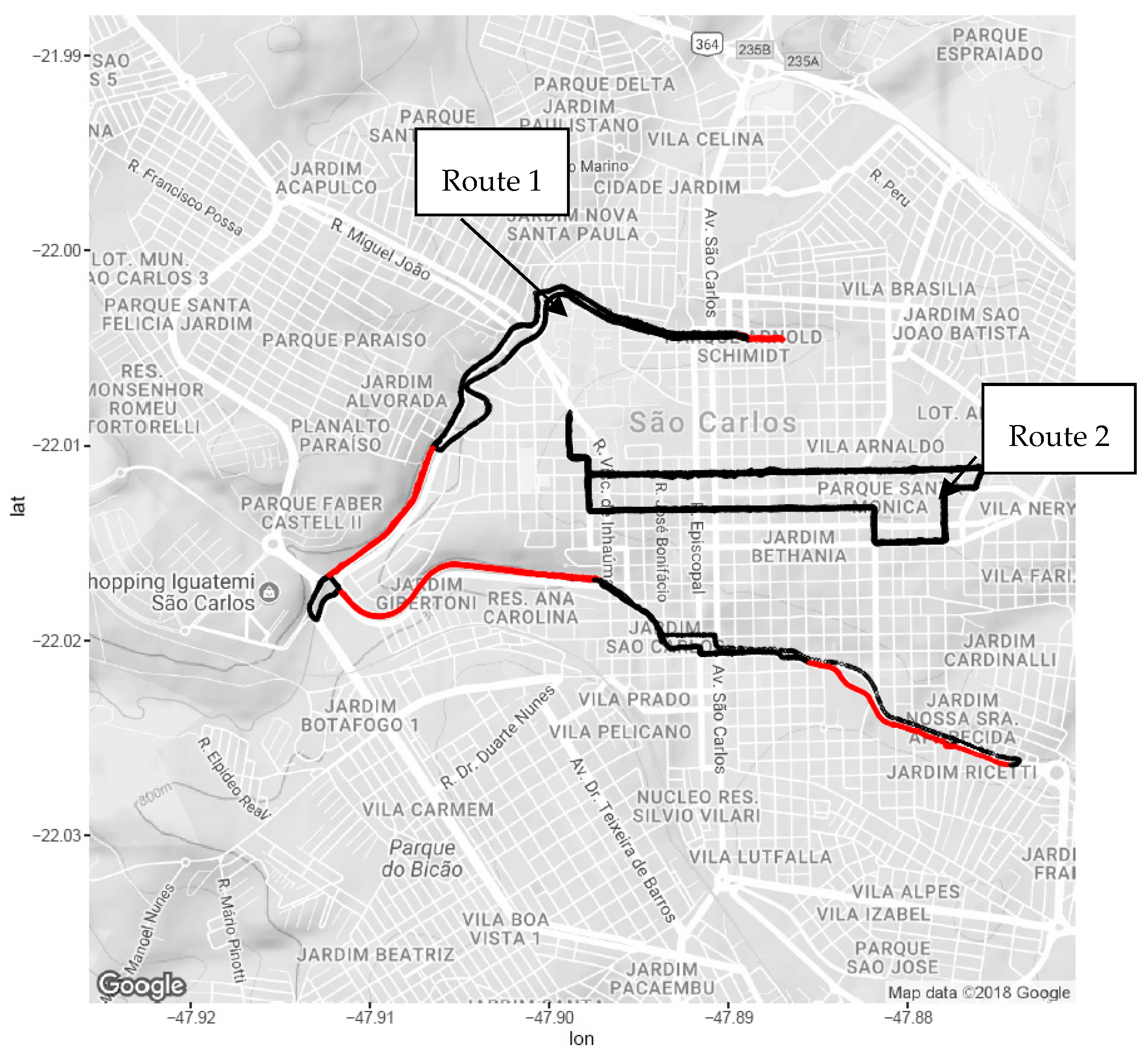
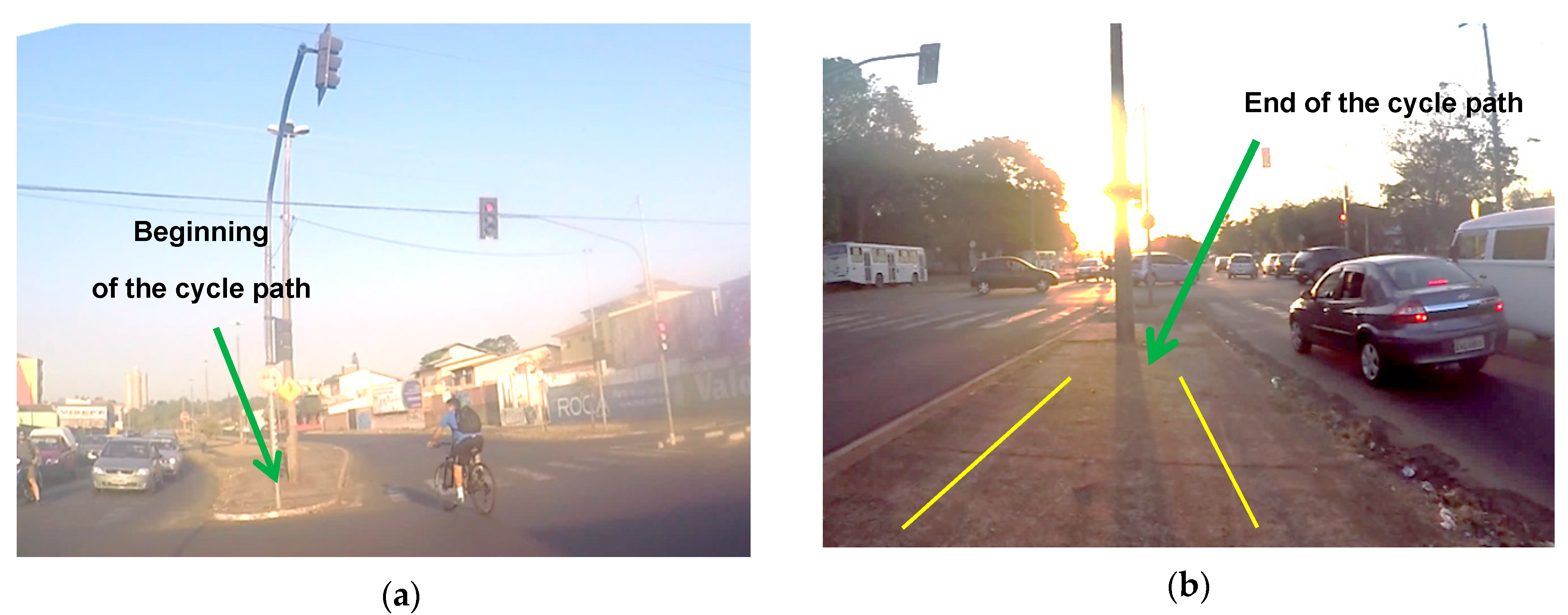
2.2. Routes Selected

The proposed method for monitoring stress and environmental characteristics was used in São Carlos, a medium-sized city (approximately 230,000 inhabitants) in the state of São Paulo, Brazil. Two routes were selected for data collection (Figure 1). Route 1 corresponds to a path of 17.1 km, which includes 4.2 km of cycle paths (red lines in Figure 1). Route 2 corresponds to a path of 5.7 km, without specially designed cycling infrastructure. The days selected for analysis were 12–14 September 2017, during the morning rush hour (between 7:00 a.m. and 9:00 a.m.) and the afternoon rush hour (between 5:00 p.m. and 7:00 p.m.).

Route 1 crosses a considerable part of the city, with segments of cycle paths disconnected from each other. This route is adjacent to a main avenue with medium traffic flow and medium speed limits. The topography of this route has medium to low slopes. Route 2 is in a central area of the city, without cycling infrastructure, and has excellent potential to attract cyclists due to the privileged location of this area in the city. This route also presents medium to low slopes. Weather conditions in São Carlos are characteristic of a humid subtropical climate zone, with an average temperature of 19.3 °C in September. Rainfall in this month is low, and during the campaign days there was no rain. The cyclists were usual riders.

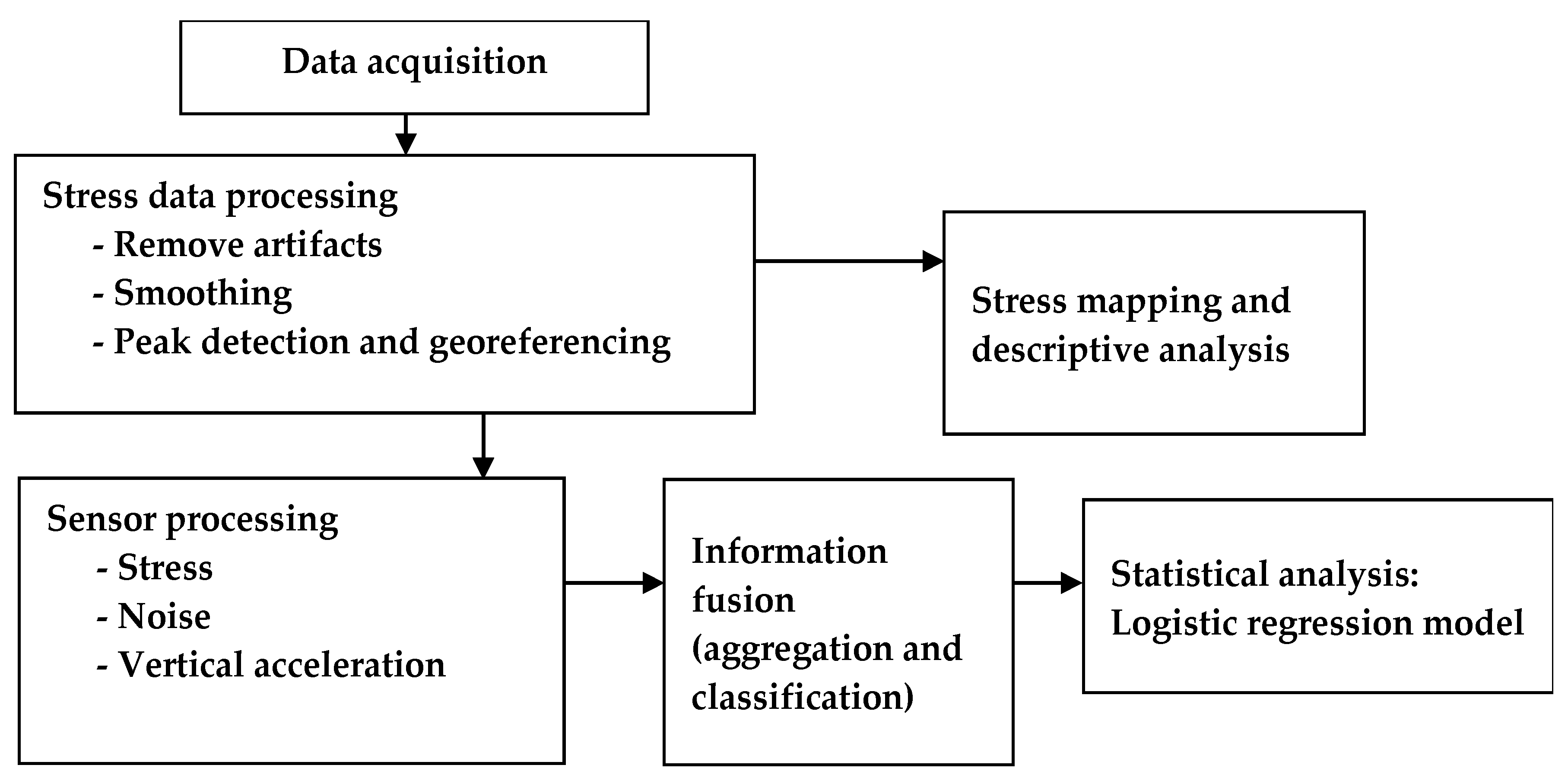
2.3. Processing and Fusing Sensor Information

In order to fuse the sensor information, the time records of the sensors, obtained separately, were matched with GPS data. The data collected in this study (over 3 days, 2 periods of the day, and 2 routes) resulted in a large number of records obtained with different acquisition rates and registered with different formats. This required advanced computational tools to ensure that obtaining the information would be carried out automatically and efficiently. In the case of noise sensor data, for example, data in text format with more than 1 million rows were classified and combined with GPS information. In order to process and fuse the information obtained from the sensors, a code was developed for reading, processing, and analyzing the data using the R program. R is a freely available language and environment for statistical computing. The general scheme of the algorithm of the program developed for processing and merging the information is presented in Figure 2. According to this scheme, first all the data of the sensors are stored, read, classified, and processed independently for each sensor. After this process, the data are mixed and aggregated over time to generate a database that will be the basis of the statistical analysis. Each stage of processing the obtained data will be explained in detail.

2.3.1. Stress Data Processing

In order to process the stress sensor data, a preprocessing phase consisting of a series of steps was performed as follows: cleaning the signal, eliminating artifacts, and smoothing the signal. After this preprocess, the skin conductance and temperature data were combined with GPS data through an algorithm implemented in the Quantum Geographic Information System (QGIS) program for peak detection and georeferencing. This algorithm generates .shp files as output with the georeferenced information of the stress peaks. The files can be imported into a geographic information system (GIS) to be analyzed later in the form of maps or combined with the information of the other sensors [63].

Stress peaks obtained from physiological measurements were calculated using the first derivative of the skin conductance and temperature. These derivatives are intended to identify whether there is an increase or decrease in the slope. To detect whether there is a peak or stress event, it is necessary to know whether the level of skin conductance is increasing; the score for this event is +1 and the skin temperature should decrease to −1. At the end of the evaluation, the 2 columns with binary data were analyzed. A peak or stress can be identified if the signal shows a decrease in skin temperature 3 s after the skin conductance level has significantly increased [16].

2.3.2. Noise Data Processing

For the noise sensor data, the algorithm steps are as follows: (1) read and classify the noise sensor data, (2) match the time records of the noise sensor and GPS data, (3) aggregate the noise levels per second, and (4) classify these levels according to

Table 1. Noise level categories (adapted from [62]).

Noise Level (LAeq (dB))	Category for the Model	Category
Less than 75	Low noise	1
75 to 85	Moderate noise	2
More than 85	Loud noise	3

[62]. To aggregate the noise data, a logarithmic sum of the sound levels was made, using the following equation:

$$LAeq=10\log {\displaystyle \sum _{i=1}^n{10}^{\left(\frac{l_i}{10}\right)}}$$

(1)

where LAeq is the value of noise aggregated by second and l_i is the ith noise value collected by the sensor.

2.3.3. Vibration Data Processing

To process the accelerometer data, the algorithm steps are as follows: (1) read the accelerometer and GPS data, (2) match the time records of the accelerometer and GPS data, (3) calculate root mean square (RMS) value per second, and (4) classify these values according to

Table 2. Comfort perceptions for different vibration levels (adapted from ISO 2631-1 [64]).

Acceptable Values of Vibration Magnitude for Comfort (RMS (m/s²))		Likely User’s Reaction	Category
As in ISO 2631-1	Values Used in This Study (to Avoid Overlapping Classes)
Less than 0.315 0.315 to 0.63 0.5 to 1 0.8 to 1.6 1.25 to 2.5 More than 2.5	Less than 0.315 0.315 to 0.63 0.63 to 1 1 to 1.6 1.6 to 2.5 More than 2.5	Not uncomfortable A little uncomfortable Fairly uncomfortable UncomfortableVery uncomfortable Extremely uncomfortable	1 2 3 4 5 6

. For the RMS calculation, the following equation was used:

$$RMS=\sqrt{\frac{1}{N}{\displaystyle \sum _{i=1}^N{x}_i{}^2}}$$

(2)

where RMS is the root mean square value, N corresponds to the N acceleration value, and x_i is the values for vertical acceleration.

Once the data from the stress, noise, and acceleration sensors were processed and combined, a unified database was constructed with the following variables: time, coordinates, noise, acceleration, presence or not of infrastructure, and time of day. This unified database was the same one used for descriptive statistical analysis and logistic regression models.

2.4. Logistic Regression Models

Logistic regression models are used to model binary responses in which there are 2 types of output: “success” or “failure.” These are types of generalized linear models (GLMs) [65], which have 3 components: (i) the random component, which is identified as the response variable and has a binomial distribution; (ii) the systematic component, which specifies the explanatory variables of the model; and (iii) the link function (in this case, the logit function, Equation (3)), which the GLM relates to the explanatory variables through a prediction equation having a linear form (Equation (4)) [66].

$$Y=\log \left(\frac{\pi }{1-\pi }\right)$$

(3)

$$Y={\beta }_0+{\beta }_1{x}_1+\dots +{\beta }_k{x}_k$$

(4)

The proposed model explores the relationship of the response to stress using 4 explanatory variables: noise, vibration, presence of cycle paths, and period of the day (morning and afternoon peak traffic times). Continuous variable noise (LAeq) and vibration (VA) were categorized according to Table 1 and Table 2 and were considered as factors in the model. The model is represented by Equation (5):

$$Y={\beta }_0+{\beta }_{1}Noise+{\beta }_{2}VA+{\beta }_{3}PCI+{\beta }_{4}Period+e$$

(5)

where LAeq corresponds to the category of noise level (Table 1), VA is vertical acceleration classified according to the category of vibration level (Table 2), PCI corresponds to the presence (1) or absence (0) of cycle paths, and Period corresponds to the period of the day (0 for the morning and 1 for the afternoon).

In logistic regression models, odds and odds ratio analyses are used to determine the importance of the explanatory variables in the model. For our model, the odds of response 1 (i.e., the presence of stress) are calculated as the exponential function of the β exponents of Equation (6):

$$\frac{\pi \left(x\right)}{1-\pi \left(x\right)}=\exp ({\beta }_0+{\beta }_{1}Noise+{\beta }_{2}VA+{\beta }_{3}PCI+{\beta }_{4}Period+e)$$

(6)

In this expression, for every 1-unit increase in X, the odds value is multiplied by e^β. Consequently, if β = 0, then e^β = 1 and the odds value does not change as X changes. To select the variables to be included in the model, on the one hand, the model considered should be complex enough to provide a better fit, but on the other hand, simpler models (with fewer variables) may be easier to interpret [66]. Based on these considerations, a selection of stepwise variables (stepwise variable selection algorithms) was implemented.

To determine the fit of the model in terms of the ability to explain the model based on the selected variables, the Cox and Snell and Nagelkerke and Akaike information criterion (AIC) techniques were used [67,68]. The Cox and Snell and Nagelkerke techniques, used to determine the fit of the logistic regression models, known as pseudo R², are similar to those used in traditional regression analyses in which R² is calculated. The adjustment values can be between 0 and 1, so that the closer to 1, the better the values fit the model.

The AIC judges a model by comparing how similar adjusted values tend to be the true expected values. An optimal model tends to have its values closest to the true probabilities of the result, that is, the model that minimizes AIC = 2 (log probability: number of parameters in the model) [66]. Thus, the lower the AIC value, the better the adjustment of the data to the model. Finally, the selected model was validated by dividing the database into two parts, one for training the model, with 70% of the data, and the other for validation, with 30%.

3. Results and Discussion

In this section, the results of applying the method to monitor stress as described above are presented. In the following subsections, maps with the results of the descriptive analysis of stress and of the logistic regression models are shown.

3.1. Stress Maps

The results of stress peaks and duration of stress (DOS) from the stress sensor can be represented and analyzed descriptively using maps. In these maps, the duration of stress can be associated with the intensity of the stress peak and can be represented in heat areas. Larger areas and more intense colors indicate higher concentrations of stress at certain points. In these points of greater intensity, considered as critical stress points, planned interventions that improve the cyclist’s comfort could be proposed. Figure 3 shows the results of the heat maps of the routes evaluated combining all the days and periods.

Figure 3 shows some highlights of high concentrations of stress where it would be interesting to make some improvements that reduce the levels of stress experienced by cyclists. Points A to D highlighted in the figure represent locations with a predominance of stress peaks in areas where the cycling infrastructure begins and ends without a transition or connection to the road. This missing connection forces an abrupt incorporation into mixed traffic, which causes high levels of stress. Actual images of these points extracted from video recordings are presented in Figure 4a. The upper left image shows a cyclist crossing the street to access the cycle path that begins at the median strip. The end of the cycling infrastructure without any connection to allow the cyclist to safely get onto the road can be observed in Figure 4a (upper right image).

In addition, the lack of safe spaces for cyclists and points of conflict at intersections (points E and F in Figure 3) can result in a high concentration of stress points. In general, high-frequency stress points were observed in the vicinity of intersections. Images at point F show the lack of space and unsafe traffic conditions for cyclists at this intersection (left and right images of Figure 4b, also captured from videos recorded during actual rides).

Table 3. Results of descriptive statistics by period of day.

Morning Rush Hour
Variable	Min.	1st	Median	Mean	3rd	Max.	σ
Stress (DOS (s))	5	5	7	9.55	12.25	28	5.70
Noise (LAeq (dB))	57.47	71.30	75.60	75.97	80.33	108.10	6.22
VA (RMS (m/s2))	0.01274	0.8736	1.142	1.431	1.621	11.62	0.99
Afternoon Rush Hour
Variable	Min.	1st	Median	Mean	3rd	Max.	σ
Stress (DOS (s))	5	6	8	10.34	11.5	43	7.60
Noise (LAeq (dB))	45.65	75.46	78.91	78.80	82.18	107.60	5.44
VA (RMS (m/s2))	0.001	0.9036	1.241	1.579	1.8	18.09	1.21

DOS, duration of stress; LAeq, noise level; VA, vertical acceleration; RMS, root mean square.

shows the results of descriptive statistics for the days selected. The results in this table include the mean, median, maximum, and minimum values, the first and third quartiles, and standard deviations, separated by morning and afternoon periods. It can be observed that the average duration of stress was 8.3% higher on average for the afternoon period, and the mean noise values were slightly higher (3.7%) in the afternoon period.

Concerning noise levels, the mean values indicate values considered to represent moderate noise (Table 1) along the routes. For vertical acceleration, it can be observed that, on average, the value was 1.5 m/s² for the two periods. This acceleration value is classified as a condition of uncomfortable vibration, as shown in Table 2.

3.2. Results of Logistic Regression Models

The results of the stress measurements were modeled from a logistic regression model as a function of the environmental variables noise (Noise), vertical acceleration (VA), presence or not of infrastructure (PCI), and period of the day (Period). A total of 19,007 records were analyzed, considering four categorical predictors: noise (three categories), vertical acceleration (six categories), presence (one) or absence (0) of cycling infrastructure, and period of the day (morning, zero; afternoon, one).

First, an analysis was carried out to determine which variables should be included in the model using a selection of stepwise variables (stepwise variable selection algorithms).

Table 4. Adjustment of logistic regression models. AIC, Aikake information criterion.

Variables	Adjustment Criteria
	Cox and Snell	Nagelkerke	AIC
Noise	7.851 × 10−5	1.25 × 10−4	19,748
VA	2.07 × 10−3	3.20 × 10−3	19,716
PCI	3.68 × 10−4	5.70 × 10−4	19,741
Period	2.06 × 10−3	3.19 × 10−3	19,708
Noise + VA	2.16 × 10−3	3.35 × 10−3	19,719
Noise + PCI	4.46 × 10−4	6.90 × 10−4	19,743
Noise + Period	2.23 × 10−3	3.45 × 10−3	19,709
VA + PCI	2.23 × 10−3	3.46 × 10−3	19,715
VA + PCI + Period	4.03 × 10−3	6.23 × 10−3	19,683
VA + Period	3.85 × 10−3	5.97 × 10−3	19,684
PCI + Period	2.42 × 10−3	3.75 × 10−3	19,704
Noise + VA + PCI	2.32 × 10−3	3.60 × 10−3	19,717
Noise + VA + PCI + Period	4.20 × 10−3	6.49 × 10−3	19,684

presents the results of adjusting the logistic regression models for each variable and combinations of variables. The adjustment was verified using the techniques proposed by Cox and Snell and Nagelkerke and AIC. In this table, lower AIC values are desirable for a good fit, and in the case of the criteria established by Cox and Snell and Nagelkerke, the closer to 1, the better the fit.

In Table 4, it can be observed that the model with all variables (Noise, VA, PCI, and Period) has the lowest AIC value and the best values of fit using the Cox and Snell and Nagelkerke criteria (4.20 × 10⁻³ and 6.49 × 10⁻³), which would put this model in first place in the selection. The model with three variables (VA, PCI, and Period) presented adjustment values similar to those of the model with all four variables (4.03 × 10⁻³ and 6.23 × 10⁻³). However, although a simpler model may be desirable, the difference between the adjustment values did not improve significantly. In addition, the model with more variables allows a more in-depth analysis of the variables that can influence stress and its importance.

Based on the above, we selected the logistic regression model that includes all variables for subsequent analysis. Regarding the validation process, after obtaining the estimated stress probabilities and classifications, the accuracy (i.e., number of correct estimates divided by total number of cases considered for validation) obtained for the selected model was 0.78%, with a 95% confidence interval equal to (0.7714, 0.793). A summary of the results obtained with the selected model is presented in

Table 5. Results of the selected logistic regression model.

Explanatory Variables	Estimate	Std. Error	z Value	Pr (>|z|)	Odds Ratio exp(β)	95% Confidence Interval for exp(β)
Intercept	−1.35361	0.12286	−11.017	<2 × 10−16	0.258306	0.201986	0.327135
Noise (LAeq (dB))
75 to 85 (Noise2)	−0.0552	0.03791	−1.456	0.1454	0.946295	0.878529	1.019304
>85 dBA (Noise3)	0.03948	0.07115	0.555	0.5790	1.040268	0.903712	1.194528
RMS (m/s²)
0.315 to 0.63 (VA2)	0.123	0.13285	0.926	0.3545	1.130885	0.874831	1.473401
0.63 to 1 (VA3)	−0.14451	0.12533	−1.153	0.2489	0.865442	0.679883	1.111831
1 to 1.6 (VA4)	−0.02449	0.12479	−0.196	0.8444	0.975804	0.767435	1.252346
1.6 to 2.5 (VA5)	0.05507	0.12754	0.432	0.6659	1.056614	0.826331	1.363036
>2.5 (VA6)	0.12673	0.12852	0.986	0.3241	1.135114	0.885927	1.467004
PCI	−0.07269	0.04071	−1.785	0.0742	0.92989	0.858353	1.006886
Period	0.21814	0.03652	5.974	2.32 × 10−9	1.243759	1.157868	1.336069

.

The importance of each variable to stress levels can be analyzed from the odds ratio values presented in Table 5. This parameter refers to the effect of each variable on the probabilities controlling the other factors. The logistic regression model obtained is:

logit[π^(x)] = −1.35361 − 0.0552*Noise2 + 0.03948*Noise3
                     + 0.123*VA2 − 0.14451*VA3 − 0.02449*VA4 + 0.05507*VA5 + 0.12673*VA6
   − 0.07296*PCI + 0.21814*Period

(7)

Even though loud noise increased the odds of experiencing stress by 4%, very uncomfortable vibrations increased the odds by 14% and the presence of cycle paths decreased the odds by 8%, the analysis of p-values and the odds ratio confidence intervals showed, with a 95% confidence level, that only the period of the day had an influence on stress, as confirmed by the data. In this case, the odds of experiencing stress increased by 24% in the afternoon rush hour compared to the morning rush hour.

4. Limitations of the Research

The findings of the study, however, were limited by the small sample. In addition to a greater number of people, more days would provide better statistical support and give more power of generalization to the conclusions.

5. Future Directions

Further studies using the methodology presented in this paper can include larger samples and subjects with different characteristics, such as gender, age, and other individual characteristics, in addition to various infrastructure types and conditions. In addition, external variables, such as weather (e.g., heat waves, rain, wind) and environmental conditions (e.g., air pollution) should be included.

6. Conclusions

A method to evaluate stress experienced by cyclists using objective measurements of physiological parameters, such as skin conductance and temperature, was proposed in this study. The main objective was to investigate the relationships between stress and noise, vibration, presence or absence of infrastructure, and period of the day. This method was validated in a medium-sized Brazilian city with only a few segments of cycling infrastructure.

Regarding the proposed methodology, this study presents contributions for planners and bicycle transport operations adopting a new approach. Unlike other approaches in which stress is inferred from the extrinsic characteristics of the cyclist (such as track width and general characteristics of the infrastructure), this new approach focuses on the perspective of monitoring parameters intrinsic to the user, such as emotions. From this perspective, stress level indicators are direct measurements of physiological responses in cyclists along cycle paths. This approach takes advantage of technological resources to extract user information through sensors and allows this information to be used in an integrated way to improve the cycling infrastructure.

Regarding the analysis of the model outcomes, the only possible conclusion was related to the period of the day. The results of the models suggest that there may be differences in stress levels between the morning peak hour and the afternoon peak hour. According to these results, the odds of experiencing stress increased by 24.3% in the afternoon peak compared to the morning peak.

References

1. Useche, S.; Montoro, L.; Alonso, F.; Oviedo-Trespalacios, O. Infrastructural and human factors affecting safety outcomes of cyclists. Sustainability 2018, 10, 229. [Google Scholar] [CrossRef]
2. Blanc, B.; Figliozzi, M. Modeling the impacts of facility type, trip characteristics, and trip stressors on cyclists’ comfort levels utilizing crowdsourced data. Transp. Res. Rec. J. Transp. Res. Board 2016, 2587, 100–108. [Google Scholar] [CrossRef]
3. Chen, C.; Anderson, J.C.; Wang, H.; Wang, Y.; Vogt, R.; Hernandez, S. How bicycle level of traffic stress correlate with reported cyclist accidents injury severities: A geospatial and mixed logit analysis. Accid. Anal. Prev. 2017, 108, 234–244. [Google Scholar] [CrossRef] [PubMed]
4. Epperson, B. Evaluating suitability of roadways for bicycle use: Toward a cycling level-of-service standard. Transp. Res. Rec. J. Transp. Res. Board 1994, 1438, 9–16. [Google Scholar]
5. Ng, A.; Kumar, A.; Heesch, K.C. Cyclist’ safety perceptions of cycling infrastructure at un-signalised intersections: Cross-sectional survey of Queensland cyclists. J. Transp. Heal. 2017, 6, 13–22. [Google Scholar] [CrossRef]
6. Sorton, A.; Walsh, T. Bicycle stress level as a tool to evaluate urban and suburban bicycle compatibility. Transp. Res. Rec. J. Transp. Res. Board 1994, 1438, 17–24. [Google Scholar]
7. Davis, J. Bicycle Safety Evaluation; Technical Report; Chattanooga Hamilton County Regional Planning Commission: Chattanooga, TN, USA, 1987. [Google Scholar]
8. Dixon, L. Bicycle and pedestrian level-of-service Performance measures and standards for congestion management systems. Transp. Res. Rec. J. Transp. Res. Board 1996, 1538, 1–9. [Google Scholar] [CrossRef]
9. Landis, B.; Vattikuti, V.; Brannick, M. Real-time human perceptions: Toward a bicycle level of service. Transp. Res. Rec. J. Transp. Res. Board 1997, 1578, 119–126. [Google Scholar] [CrossRef]
10. Turner, S.M.; Shafer, C.S.; Stewart, W.P. Bicycle Suitability Criteria for State Roadways in Texas; Summary Report; Texas Transportation Institute: College Station, TX, USA, 1997; p. 95. [Google Scholar]
11. Jensen, S. Pedestrian and bicyclist level of service on roadway segments. Transp. Res. Rec. J. Transp. Res. Board 2007, 2031, 43–51. [Google Scholar] [CrossRef]
12. Transportation Research Board of the National Academies. Transportation Reseach Board. HCM-Highway Capacity Manual, 5th ed.; Transportation Research Board of the National Academies: Washington, DC, USA, 2010; ISBN 978-0-309-16080. [Google Scholar]
13. Mekuria, M.C.; Furth, P.G.; Nixon, H. Low-Stress Bicycling and Network Connectivity. Available online: https://nacto.org/wp-content/uploads/2017/11/1005-low-stress-bicycling-network-connectivity.pdf (accessed on 5 July 2018).
14. Wang, H.; Palm, M.; Chen, C.; Vogt, R.; Wang, Y. Does bicycle network level of traffic stress (LTS) explain bicycle travel behavior? Mixed results from an Oregon case study. J. Transp. Geogr. 2016, 57, 8–18. [Google Scholar] [CrossRef]
15. Fitch, D.T.; Sharpnack, J.; Handy, S. The Road Environment and Bicyclists’ Psychophysiological Stress. In Proceedings of the 6th Annual International Cycling Safety Conference, Davis, CA, USA, 21–22 September 2017; pp. 22–24. [Google Scholar]
16. Zeile, P.; Resch, B.; Loidl, M.; Petutschnig, A. Urban Emotions and Cycling Experience—Enriching Traffic Planning for Cyclists with Human Sensor Data. GI_Forum J. Geogr. Inf. Sci. 2016, 1, 204–216. [Google Scholar] [CrossRef]
17. Caviedes, A.; Technology, T.; Technology, T.; Le, H.; Feng, W. What does stress real-world cyclists? In Proceedings of the Transportation Research Board 96th Annual Meeting, Washington, DC, USA, 8–12 January 2017; pp. 1–15. [Google Scholar]
18. Liu, F.; Figliozzi, M. Utilizing Egocentric Video and Sensors to Conduct Naturalistic Bicycling Studies; Technical Report; NITC-RR-805; Transportation Research and Education Center (TREC): Portland, OR, USA, 2016. [Google Scholar]
19. Zeile, P.; Resch, B.; Exner, J.P.; Sagl, G. Urban emotions: Benefits and risks in using human sensory assessment for the extraction of contextual emotion information in urban planning. In Planning Support Systems and Smart Cities; Geertman, S., Ferreira, J., Jr., Goodspeed, R., Stillwell, J., Eds.; Springer: Cham, Switzerland, 2015; Volume 213, pp. 209–225. [Google Scholar]
20. Ulrich-Lai, Y.M.; Herman, J.P. Neural regulation of endocrine and autonomic stress responses. Nat. Rev. Neurosci. 2009, 10, 397–409. [Google Scholar] [CrossRef] [PubMed] [Green Version]
21. Bergner, B.; Zeile, P.; Papastefanou, G. Emotionales Barriere-GIS als neues Instrument zur Identifikation und Optimierung stadträumlicher Barrieren. Available online: https://gispoint.de/fileadmin/user_upload/paper_gis_open/AGIT_2011/537508010.pdf (accessed on 5 July 2018).
22. Kreibig, S.D. Autonomic nervous system activity in emotion: A review. Biol. Psychol. 2010, 84, 14–41. [Google Scholar] [CrossRef] [PubMed]
23. Yang, C.; Wu, C. Primary or secondary tasks? Dual-task interference between cyclist hazard perception and cadence control using cross-modal sensory aids with rider assistance bike computers. Appl. Ergon. 2017, 59, 65–72. [Google Scholar] [CrossRef] [PubMed]
24. Evans, G.W.; Wener, R.E. Rail commuting duration and passenger stress. Heal. Psychol. 2006, 25, 408–412. [Google Scholar] [CrossRef] [PubMed]
25. Kaplan, S.; Prato, C.G. “Them or Us”: Perceptions, cognitions, emotions, and overt behavior associated with cyclists and motorists sharing the road. Int. J. Sustain. Transp. 2016, 10, 193–200. [Google Scholar] [CrossRef] [Green Version]
26. Joshi, M.S.; Senior, V.; Smith, G.P. A diary study of the risk perceptions of road users. Heal. Risk Soc. 2001, 3, 261–279. [Google Scholar] [CrossRef]
27. Szalma, J.L.; Hancock, P.A. Noise effects on human performance: A meta-analytic synthesis. Psychol. Bull. 2011, 137, 682–707. [Google Scholar] [CrossRef] [PubMed]
28. Hockey, G.R.J.; Hamilton, P. Arousal and Information Selection in Short-term Memory. Nature 1970, 226, 866–867. [Google Scholar] [CrossRef] [PubMed]
29. Boman, E.; Enmarker, I.; Hygge, S. Strength of noise effects on memory as a function of noise source and age. Noise Heal. 2005, 7, 11–26. [Google Scholar] [CrossRef]
30. Barbosa, A.S.M.; Cardoso, M.R.A. Hearing loss among workers exposed to road traffic noise in the city of São Paulo in Brazil. Auris Nasus Larynx 2005, 32, 17–21. [Google Scholar] [CrossRef] [PubMed]
31. Babisch, W. Cardiovascular effects of noise. Noise Heal. 2011, 13, 201–204. [Google Scholar] [CrossRef] [PubMed]
32. Babisch, W.; Beule, B.; Schust, M.; Kersten, N.; Ising, H. Traffic noise and risk of myocardial infarction. Epidemiology 2005, 16, 33–40. [Google Scholar] [CrossRef] [PubMed]
33. Brown, A.L.; Muhar, A. An approach to the acoustic design of outdoor space. J. Environ. Plan. Manag. 2004, 47, 827–842. [Google Scholar] [CrossRef]
34. Lavandier, C.; Defréville, B. The contribution of sound source characteristics in the assessment of urban soundscapes. Acta Acust. United Acust. 2006, 92, 912–921. [Google Scholar]
35. Nilsson, M.E.; Berglund, B. Soundscape quality in suburban green areas and city parks. Acta Acust. United Acust. 2006, 92, 903–911. [Google Scholar]
36. Venkatappa, K.G.; Vinutha Shankar, M.S. Study of association between noise levels and stress in traffic policemen of Bengaluru city. Biomed. Res. 2012, 23, 135–138. [Google Scholar]
37. Michaud, D.; Keith, S.; McMurchy, D. Noise annoyance in Canada. Noise Heal. 2005, 7, 39–47. [Google Scholar] [CrossRef]
38. Öhrström, E. Longitudinal surveys on effects of changes in road traffic noise—Annoyance, activity disturbances, and psycho-social well-being. J. Acoust. Soc. Am. 2004, 115, 719–729. [Google Scholar] [CrossRef] [PubMed]
39. Öhrström, E.; Skånberg, A.; Svensson, H.; Gidlöf-Gunnarsson, A. Effects of road traffic noise and the benefit of access to quietness. J. Sound Vib. 2006, 295, 40–59. [Google Scholar] [CrossRef]
40. Björk, J.; Ardö, J.; Stroh, E.; Lövkvist, H.; Östergren, P.O.; Albin, M. Road traffic noise in southern Sweden and its relation to annoyance, disturbance of daily activities and health. Scand. J. Work. Environ. Heal. 2006, 32, 392–401. [Google Scholar] [CrossRef] [Green Version]
41. Ramos, T.D.C. Avaliação da Exposição de Ciclistas ao Ruído em uma Cidade Média Brasileira. Master’s Thesis, University of São Paulo, São Paulo, Brazil, 2017. [Google Scholar]
42. Apparicio, P.; Carrier, M.; Gelb, J.; Séguin, A.M.; Kingham, S. Cyclists’ exposure to air pollution and road traffic noise in central city neighbourhoods of Montreal. J. Transp. Geogr. 2016, 57, 63–69. [Google Scholar] [CrossRef]
43. Dupuisl, H.; Gemne, G. Hand-arm vibration and the central nervous system. Int. Arch. Occup. Environ. Health 1985, 55, 185–189. [Google Scholar] [CrossRef]
44. Putz-Anderson, V.; Bernard, B.; Burt, S. Musculoskeletal Disorders and Workplace Factors—A Critical Review of Epidemiologic Evidence for Work-Related Musculoskeletal Disorders of the Neck, Upper Extremity, and Low Back; National Institute for Occupational Safety and Health: Columbia Parkway Cincinnati, OH, USA, 1997. [Google Scholar]
45. Griffin, M.J.; Bovenzi, M. The diagnosis of disorders caused by hand-transmitted vibration: Southampton Workshop 2000. Int. Arch. Occup. Environ. Health 2002, 75, 1–5. [Google Scholar] [CrossRef] [PubMed]
46. Parkin, J.; Sainte Cluque, E. The impact of vibration on comfort and bodily stress while cycling. In Proceedings of the UTSG 46th Annual Conference, Newcastle, UK, 6–8 January 2014; UWE: Newcastle, UK, 2014; pp. 6–8. [Google Scholar]
47. Torbic, D.; Elefteriadou, L.; El-Gindy, M. Methodology for Evaluating Impacts of Rumble Strips on Bicyclists. In Transportation Research Board 82nd Annual Meeting; TRB, Ed.; Transportation Research Board of the National Academies: Washington, DC, USA, 2003; p. 24. [Google Scholar]
48. Levy, M.; Smith, G.A. Effectiveness of vibration damping with bicycle suspension systems. Sport. Eng. 2005, 8, 99–106. [Google Scholar] [CrossRef]
49. Yamanaka, H. Measuring Level-of-Service for Cycling of Urban Streets Using “Probe Bicycle System”. Transportation 2007, 7, 1614–1625. [Google Scholar]
50. Du, W.; Zhang, D.; Zhao, X. Dynamic modelling and simulation of electric bicycle ride comfort. In Proceedings of the International Conference on Mechatronics and Automation, Changchun, China, 9–12 August 2009; pp. 4339–4343. [Google Scholar] [CrossRef]
51. Giubilato, F.; Petrone, N. A method for evaluating the vibrational response of racing bicycles wheels under road roughness excitation. Procedia Eng. 2012, 34, 409–414. [Google Scholar] [CrossRef]
52. Olieman, M.; Marin-Perianu, R.; Marin-Perianu, M. Measurement of dynamic comfort in cycling using wireless acceleration sensors. Procedia Eng. 2012, 34, 568–573. [Google Scholar] [CrossRef]
53. Arpinar-Avsar, P.; Birlik, G.; Sezgin, Ö.C.; Soylu, A.R. 14_The effects of surface-induced loads on forearm muscle activity during steering a bicycle. J. Sport. Sci. Med. 2013, 12, 512–520. [Google Scholar]
54. Macdermid, P.W.; Fink, P.W.; Stannard, S.R. Transference of 3D accelerations during cross country mountain biking. J. Biomech. 2014, 47, 1829–1837. [Google Scholar] [CrossRef] [PubMed]
55. Ayachi, F.S.; Dorey, J.; Guastavino, C. Identifying factors of bicycle comfort: An online survey withenthusiast cyclists. Appl. Ergon. 2015, 46, 124–136. [Google Scholar] [CrossRef] [PubMed]
56. Chou, C.-P.; Lee, W.-J.; Chen, A.-C.; Wang, R.-Z.; Tseng, I.-C.; Lee, C.-C. Simulation of Bicycle-Riding Smoothness by Bicycle Motion Analysis Model. J. Transp. Eng. 2015, 141, 04015031. [Google Scholar] [CrossRef]
57. Thigpen, C.G.; Li, H.; Handy, S.L.; Harvey, J. Modeling the Impact of Pavement Roughness on Bicycle Ride Quality. Transp. Res. Rec. J. Transp. Res. Board 2015, 2520, 67–77. [Google Scholar] [CrossRef]
58. Takahashi, J.; Kobana, Y.; Tobe, Y.; Lopez, G. Classification of Steps on Road Surface Using Acceleration Signals. In Proceedings of the 12th EAI International Conference on Mobile and Ubiquitous Systems: Computing, Networking and Services, Coimbra, Portugal, 22–24 July 2015. [Google Scholar]
59. Ambrož, M. 30-Raspberry Pi as a low-cost data acquisition system for human powered vehicles. Measurement 2017, 100, 7–18. [Google Scholar] [CrossRef]
60. Zeile, P. Urban Emotions. Available online: http://urban-emotions.com/?author=2 (accessed on 20 March 2018).
61. Dekoninck, L.; Botteldooren, D.; Panis, L.I.; Hankey, S.; Jain, G.; Karthik, S.; Marshall, J. Applicability of a noise-based model to estimate in-traffic exposure to black carbon and particle number concentrations in different cultures. Environ. Int. 2014, 74, 89–98. [Google Scholar] [CrossRef] [PubMed] [Green Version]
62. Ramos, T.C.; Rodrigues da Silva, A.N.; De Souza, L.C.L.; Dekoninck, L.; Botteldooren, D. Assessing noise exposure levels along recently built cyclepaths in a Brazilian city with a mobile sensing system. In Proceedings of the CUPUM 2015—14th International Conference on Computers in Urban Planning and Urban Management, Cambrige, MA, USA, 7–10 July 2015; Massachusetts Institute of Technology: Cambrige, MA, USA, 2015. [Google Scholar]
63. Beyel, S.; Wilhelm, J.; Mueller, C.; Zeile, P.; Klein, U. Stresstest städtischer Infrastrukturen—Ein Experiment zur Wahrnehmung des Alters im öffentlichen Raum. In Proceedings of the 21st International Conference on Urban Planning, Regional Development and Information Society, Hamburg, Germany, 22–24 June 2016; Available online: https://www.corp.at/archive/CORP2016_42.pdf (accessed on 5 July 2018).
64. International Standards Organization ISO 2631-1. Mechanical Vibration and Shock-Evaluation of Human Exposure to Whole-Body Vibration—Part 1—General Requirements; ISO-Standards Cat.: Geneva, Switzerland, 1997; Volume 31. [Google Scholar]
65. McCullagh, P.; Nelder, J.A. Generalized linear models, no. 37. In Monograph on Statistics and Applied Probability; CRC Press: Boca Raton, FL, USA, 1989. [Google Scholar]
66. Agresti, A. An Introduction to Categorical Data Analysis, 2nd ed.; Wiley: Gainesville, FL, USA, 2007; ISBN 9780471226185. [Google Scholar]
67. Cox, D.R.; Snell, D.J. The Analysis of Binary Data, 2nd ed.; Chapman & Hall: London, UK, 1989. [Google Scholar]
68. Nagelkerke, N.J.D. A note on a general definition of the coefficient of determination. Biometrika 1991, 78, 691–692. [Google Scholar] [CrossRef]
Figure 1. Routes selected for data collection (red lines indicate sections with specially designed cycling infrastructure, e.g., cycle ways or paths).
Sustainability 10 02379 g001
Figure 2. Processing and fusion of sensor data.
Sustainability 10 02379 g002
Figure 3. Heat stress map areas resulting from the combination of all the days and periods analyzed. Larger areas and darker colors indicate higher concentrations of stress at certain points.
Sustainability 10 02379 g003
Figure 4. Images of critical stress points. (a) Detail of point A in Figure 3: cyclist crossing the street to access the cycle path. (b) Detail of point A in Figure 3: cycling infrastructure without any connection. Details of point F in Figure 3: (c) points of conflict at an intersection and (d) lack of space to accommodate bicycles.
Sustainability 10 02379 g004aSustainability 10 02379 g004b