Decomposition Analysis of Carbon Emissions from Energy Consumption in Beijing-Tianjin-Hebei, China: A Weighted-Combination Model Based on Logarithmic Mean Divisia Index and Shapley Value

Abstract

The Beijing-Tianjin-Hebei (B-T-H) region, who captures the national strategic highland in China, has drawn a great deal of attention due to the fog and haze condition and other environmental problems. Further, the high carbon emissions generated by energy consumption has restricted its further coordinated development seriously. In order to accurately analyze the potential influencing factors that contribute to the growth of energy consumption carbon emissions in the B-T-H region, this paper uses the carbon emission coefficient method to measure the carbon emissions of energy consumption in the B-T-H region, using a weighted combination based on Logarithmic Mean Divisia Index (LMDI) and Shapley Value (SV). The effects affecting carbon emissions during 2001–2013 caused from five aspects, including energy consumption structure, energy consumption intensity, industrial structure, economic development and population size, are quantitatively analyzed. The results indicated that: (1) The carbon emissions had shown a sustained growth trend in the B-T-H region on the whole, while the growth rates varied in the three areas. In detail, Hebei Province got the first place in carbon emissions growth, followed by Tianjin and Beijing; (2) economic development was the main driving force for the carbon emissions growth of energy consumption in B-T-H region. Energy consumption structure, population size and industrial structure promoted carbon emissions growth as well, but their effects weakened in turn and were less obvious than that of economic development; (3) energy consumption intensity had played a significant inhibitory role on the carbon emissions growth; (4) it was of great significance to ease the carbon emission-reduction pressure of the B-T-H region from the four aspects of upgrading industrial structure adjustment, making technological progress, optimizing the energy structure and building long-term carbon-emission-reduction mechanisms, so as to promote the coordinated low-carbon development.

1. Introduction

With the rapid development of the economy, China is now facing a severe energy and environment situation with issues such as increasing energy consumption, enormous carbon emissions, serious fog and haze conditions and frequent extreme weather disasters. As a responsible country in the world, the Chinese government has clarified the importance and necessity of low-carbon development and has issued clear energy-saving and emission-reduction goals in the national plan for future development in the form of a decree. For instance, carbon emissions per unit of gross domestic product (GDP) in 2020 would be decreased by 40% to 45% compared to that in 2005. Obviously, China has regarded energy conservation, emission reduction, and low-carbon development as important national strategies [1,2]. However, the achievements gained at present are not obvious enough and there exists great room for further study and exploration. The Beijing-Tianjin-Hebei (B-T-H) region, followed to the “Yangtze River Delta” and “Pearl River Delta”, have developed to be the third major economic circle, however, there are still many problems such as carbon emissions, frog and haze conditions, pollution and energy problems, which are much more serious than that in the other two economic circles [3]. According to the reports of China National Environmental Monitoring Centre, during January to June in 2013, the proportion of days when the air quality dropped to healthy levels in the B-T-H region accounted for only 31%, which was 24% less than that of the national average. As for the serious pollution days, it took up 26.2% of the 180 days, 15.2% higher than that of the national average. In addition, seven cities who are members of the B-T-H region entered the top 10 serious polluted cities nationwide [4]. Relevant research and practice shows that the rapid growth of energy consumption is one of the important sources of air pollution, so that strictly controlling the total energy consumption is crucial to improve energy efficiency and achieve low-carbon economic development. At present, with the deepening collaborative development from the initial idea to the specific implementation strategy today, the B-T-H region has come together through a period of history, but the carbon emissions resulting from energy consumption still remains at a high level that seriously restricts regional “resource saving and environment-friendly” construction[5,6]. In this context, the analysis of carbon emissions and influencing factors benefits us to understand the carbon emissions situation in the B-T-H region as a whole, so as to provide important suggestions for its collaborative development planning.

Based on the “2006 IPCC national greenhouse gas inventory guide” of carbon accounting methods, Wu and Zhao [7] calculated the carbon dioxide emissions, emissions intensity, per capita emissions and emissions per unit area of B-T-H in 2000–2011, and analyzed energy consumption, carbon emissions and economic growth of B-T-H from the perspectives of change trend, consumption structure, correlation and spatial distribution. Feng and Li [8] chose 13 cities in the B-T-H region as the research object and focused on the carbon dioxide emission efficiency and reduction potential of each city, to provide a reference for peak emissions. Using China’s 30 provinces interregional input-output table and industrial carbon emissions data in 2007 and 2010, Yan [9] built a multiregional input-output-structural decomposition analysis model to estimate the trends of carbon footprint in B-T-H region and its drivers. Piao and Li [10] constructed an evaluation index system for regional carbon reduction ability with five aspects of carbon reduction factors. By applying the comprehensive evaluation model based on entropy value method, the states of carbon reduction ability of B-T-H from 2001 to 2011 were analyzed, and based on the results, they proposed the cooperation carbon reduction strategy of B-T-H region. In summary, there is currently no research on the factors affecting the carbon emissions of energy consumption in the B-T-H region, and this is the key to realizing the energy-saving and emission-reduction strategy in the B-T-H region. Therefore, it is necessary to conduct research on the factors affecting the carbon emissions of energy consumption in the B-T-H region.

At present, there are many methods to measure carbon emissions, among which the practical survey method, model method, material balance algorithm and direct carbon emissions coefficient method are commonly used. The practical survey method is a method which uses the statistical data admitted by environmental authorities to estimate the greenhouse gases generated from raw coal, oil, natural gas and other energy forms [11]. The model method is to calculate the carbon emissions of the region by establishing a mathematical model such as the MARKAL model [12], the AIM model [13] and the Logistic model [14]. The material balance algorithm makes the law of conservation of mass as its basic principle to quantitatively analyze the materials in the production process, mainly including the up-bottom accounting form [15] and the bottom-up accounting form [16,17,18], where the former is the recommended method by the Intergovernmental Panel on Climate Change (IPCC). The direct carbon emissions coefficient method to measure emissions is mainly based on the total consumption of all energy forms in different industries and the carbon emission coefficient of different energy forms [19]. Among these methods, the practical survey method is dependent on high-tech monitoring equipment, which is confronted with obstacles for implementation because of the high cost and enormous samples. Similar to the material balance algorithm, although the accuracy of the calculation result is relatively high, the model method is limited not only for requiring a large amount of data as a basis, but also for being complex to calculate, which makes it hard to get results in a short time. As for the direct carbon emissions coefficient method which highly relies on the carbon emission coefficient, it is much more suitable for measuring carbon emissions from energy consumption in the B-T-H region either because of the simple and practicable calculation or lower data requirements.

From the perspective of decomposition methods, Structural Decomposition Analysis (SDA), Index Decomposition Analysis (IDA), Mean Ratio Change Index (MRCI), and Shapley value (SV) method are commonly used. The SDA is based on the consumption coefficient matrix, which uses an input-output table to carry out detailed researches on the impact of factors, mainly including the input-output method and the bipolar decomposition method [20,21]. The IDA works through transforming a study object into a number of factors in the form of product by mathematical formulas, and then calculates the incremental impact of factors, mainly including the Laspeyres decomposition method [22] and Divisia decomposition method [23]. The Logarithmic Mean Divisia (LMDI) decomposition method, using the logarithmic mean formula instead of the traditional arithmetic average formula to calculate the weights, is now the development and refinement of the Index Decomposition Analysis, which is proposed by Ang B.W. and is the most widely-used method in the field of carbon emission decomposition analysis [24]. The MRCI takes the proportion of the average change rate of each factor as the weight, then calculates the effects of decomposition factors [25]. The SV method, as an emerging decomposition method, was used to deal with the problem of cooperative game at first. Shorrocks then introduced Shapley’s Value to solve the problem of decomposition analysis since it is in agreement with the cooperative game [26]. Through the contrastive analysis, it can be seen that the SDA highly depends on the input-output table, requiring enormous and complex data. The Laspeyres decomposition method and Divisia decomposition method suffers from the shortcoming of zero or residual error, which results in a large deviation in the decomposition results caused by insufficient explanation of the factors. In contrast, the LMDI method, the MRCI method and the SV method are superior for no residual error. Among them, the MRCI method is weaker than the other two methods in theory application, and the validity of this method remains to be verified. The LMDI decomposition method is more advanced not only because it focuses on multiple factors, but also because its decomposition results can be in additive form or in multiplied form without residual error. Besides, it can also be used for some incomplete data sets, effectively improving the interpretability of influencing factors, which brings the great facility in the field of energy and environmental problems analysis [27,28]. However, this method has weakness for lacking clear economic significance. In this respect, the SV method overwhelms the LMDI for effective economic implications in a cooperative game. Using this method, the sum of the influences of factors is equal to the change values of the decomposed variables to avoid the residual error, and the calculating results reflect the average marginal contribution of all the members to the cooperative coalition [29,30]. However, in the study of carbon emission decomposition analysis, different factors in the cooperative coalition change in different directions, making the coalition lack stability, which to some extent weakens the interpretability of the SV method. Therefore, combining the LMDI decomposition method with the SV method to carry out the analysis in the B-T-H region is more accurate and reasonable.

Based on what has been introduced above, in this paper, the carbon emissions from energy consumption and its influencing factors during 2000–2013 in the B-T-Hi region were studied, so as to provide suggestions for the economic circle. In particular, first, the direct carbon emissions coefficient method was utilized to measure the carbon emissions of 25 types of energy forms in the B-T-H region. Secondly, the weighted-combination decomposition analysis model which was made up by the LMDI based on the Kendall coordination coefficient and the SV method was established to analyze the factors influencing carbon emissions. Finally, according to the decomposition results, the corresponding measures and suggestions were put forward. The innovation of this paper is to use the weighted combination model to decompose the influencing factors of B-T-H energy consumption carbon emissions, making full use of the advantages of the LMDI method and Shapley value method, while domestic and foreign scholars generally use LMDI method or Shapley value method for carbon emission alone. The comprehensive application of the two methods achieves complementary advantages, improves the credibility of the calculation results, finds the main influencing factors, and facilitates the more accurate decomposition research of the influencing factors. The rest of the paper is structured as follows: Section 2 estimated the carbon emissions from energy consumption in the B-T-H region; Section 3 established the carbon emission decomposition model; then thorough analysis was made aiming at the decomposition results and corresponding measures and suggestions were proposed for energy saving and emission reduction in Section 4; at last, Section 5 summarized the research results.

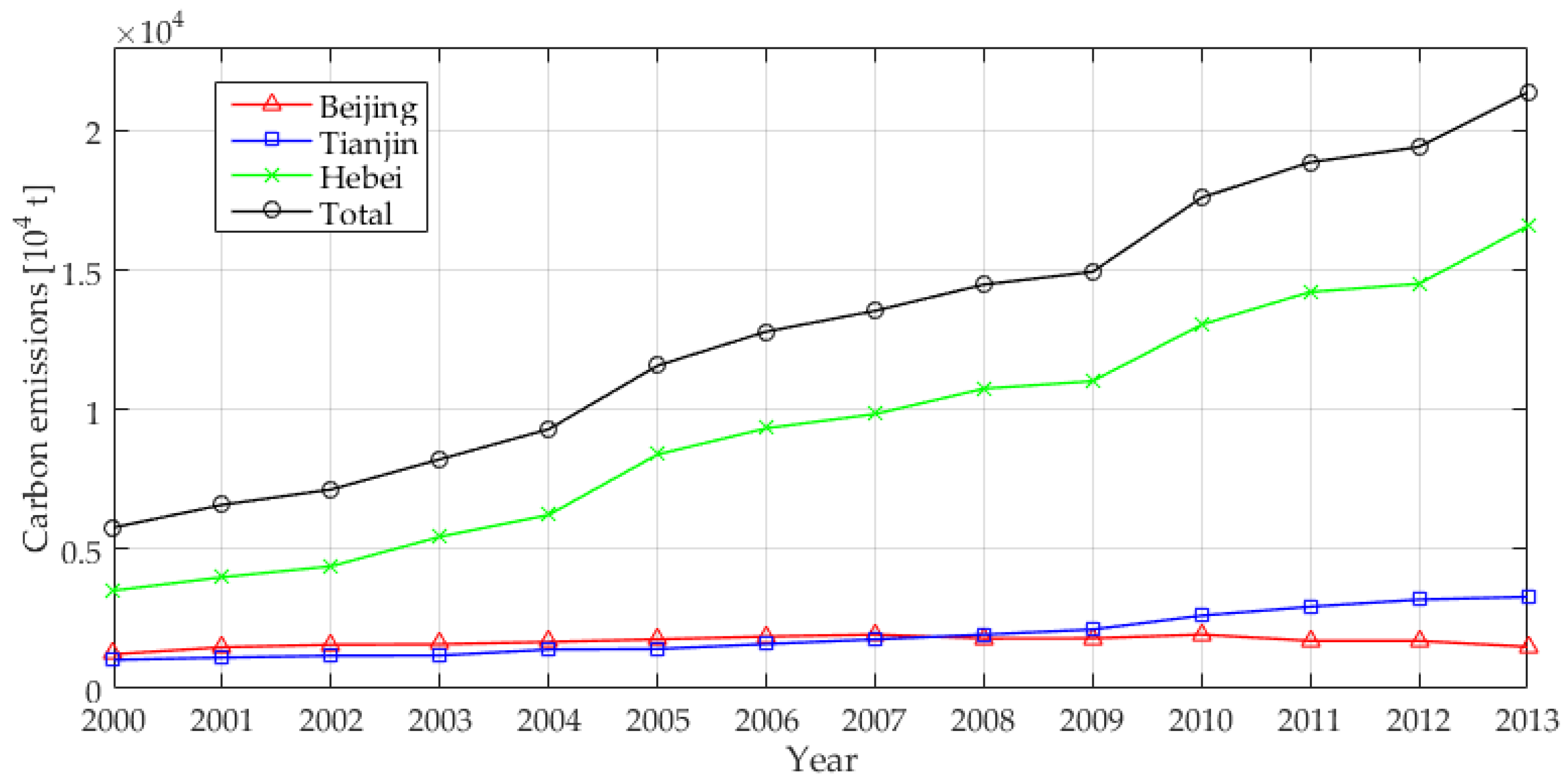
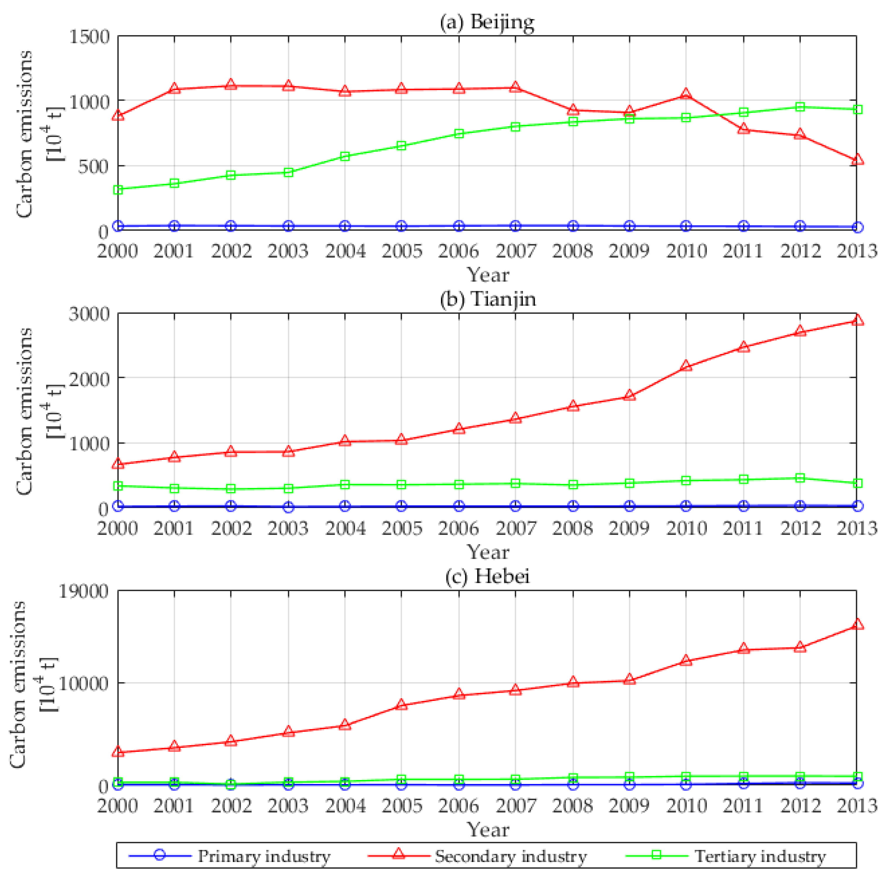
2. Measurement of Carbon Emissions from Energy Consumption

The direct carbon emissions coefficient method is utilized to measure the carbon emissions from energy consumption in the B-T-H region. The formula is as follows [15]:

$$CE={\displaystyle \sum _{i=1}^n{\displaystyle \sum _{j=1}^m{E}_{ij}\times SS{C}_j\times CE{C}_j}}$$

(1)

where $CE$ means the total carbon emissions; $E_{ij}$ means the amount of the jth energy form of the ith sector; $SS{C}_j$ means the standard coal coefficient of the jth energy form; $CE{C}_j$ means the carbon emissions coefficient of the jth energy form which is calculated by formula (2) [15]:

$$CE{C}_j=NC{V}_j\times CC{V}_j\times CO{R}_j\times 44/12$$

(2)

where $NC{V}_j$ means the net calorific value of the jth energy form; $CC{V}_j$ means the carbon content per unit calorific value of the jth energy form; $CO{R}_j$ means the carbon oxidation rate of the jth energy form, in the actual process of energy consumption, the carbon element cannot completely be converted to greenhouse gas, but its proportion is relatively small, therefore, in order to simplify the calculation, we assume that all the fuel converts into the greenhouse gases, that is to say, 100% of fuel is l oxidized; $44/12$ means the amount of the carbon element in the carbon dioxide.

In order to fully reflect the carbon emission condition from energy consumption in the B-T-H region, in this paper, the data of three major industries is set as the analysis basis. Among them, the primary industry includes agriculture, forestry, animal husbandry and fishery without corresponding service industry; the secondary industry refers to the mining industry (excluding mining auxiliary activities), manufacturing (excluding metal products, machinery and equipment repair industry), electricity, heat, gas and water production and supply industry, and construction industry; the tertiary industry, in other words, the service industry, is composed of the sectors who are not included in the other two industries. In the light of the types of energy listed in the China Energy Statistical Yearbook [31], 25 types of energy forms are selected to be analyzed, including raw coal, clean coal, other washing coal, briquette, coke, coking gas, blast furnace gas, converter gas, other gas, other carbonized products, crude oil, gasoline, kerosene, diesel oil, fuel oil, naphtha, grease oil, paraffin, solvent oil, oil asphalt, petroleum, liquefied petroleum gas, refinery gas, other petroleum products and natural gas. The time span is from 2000 to 2013, when China completed the “Ninth Five-Year Plan” in 2000, thus this year can be used as the benchmark year; 2013 is the year when the China Energy Statistical Yearbook published the latest data. The standard coal coefficient of all energy forms and other parameters can be consulted in Appendix A (

Table A1. The carbon emissions in the B-T-H region are as follows: (10 thousand tons).

Year	Beijing			Tianjin			Hebei
	Primary Industry	Secondary Industry	Tertiary Industry	Primary Industry	Secondary Industry	Tertiary Industry	Primary Industry	Secondary Industry	Tertiary Industry
2000	35.64	877.30	318.28	21.99	666.49	340.01	61.56	3170.95	282.58
2001	39.14	1084.33	359.92	27.85	775.36	307.76	57.30	3648.82	288.06
2002	38.07	1111.11	424.41	31.22	857.96	289.15	40.70	4229.06	115.97
2003	36.60	1108.66	446.09	20.17	862.80	303.35	50.14	5090.66	302.57
2004	36.20	1066.81	570.60	22.53	1018.36	359.57	47.77	5797.21	381.59
2005	34.90	1081.79	649.93	26.39	1035.80	356.51	62.57	7749.96	580.81
2006	37.66	1086.82	742.60	26.17	1207.28	365.00	36.04	8720.37	577.53
2007	39.27	1096.32	800.89	27.30	1362.88	374.89	40.16	9209.85	592.15
2008	38.98	924.57	833.29	27.14	1556.28	352.72	64.17	9920.47	768.32
2009	36.22	906.34	858.91	29.02	1707.19	383.12	62.93	10,168.98	788.81
2010	34.84	1038.49	864.97	31.79	2163.04	420.21	88.74	12,073.90	884.05
2011	34.31	774.74	904.35	35.58	2465.70	434.40	174.02	13,149.00	897.56
2012	32.19	730.24	948.72	38.81	2692.86	458.41	246.93	13,362.15	905.95
2013	30.48	537.44	931.47	33.81	2872.01	381.44	215.74	15,490.85	882.74

,

Table A2. The total carbon emissions in the B-T-H region are as follows: (10 thousand tons).

Year	Beijing	Tianjin	Hebei	Total
2000	1231.22	1028.50	3515.09	5774.81
2001	1483.39	1110.97	3994.19	6588.55
2002	1573.58	1178.33	4385.73	7137.64
2003	1591.35	1186.32	5443.37	8221.04
2004	1673.60	1400.46	6226.56	9300.62
2005	1766.62	1418.70	8393.35	11,578.67
2006	1867.08	1598.46	9333.94	12,799.48
2007	1936.48	1765.07	9842.17	13,543.72
2008	1796.84	1936.13	10,752.96	14,485.93
2009	1801.47	2119.33	11,020.72	14,941.52
2010	1938.29	2615.05	13,046.69	17,600.03
2011	1713.40	2935.67	14,220.58	18,869.65
2012	1711.15	3190.08	14,515.03	19,416.26
2013	1499.39	3287.26	16,589.33	21,375.98

,

Table A3. The calculation parameters of carbon emissions in this study are as follows:

Energy Type	SSC [kg SC/kg]	NCV [MJ/t or MJ/104 m3]	CCV [g C/MJ]	CEC [t C/t or t C/104 m3]
Raw coal	0.7143	20,908.42	26.37	0.5514
Clean coal	0.9000	26,344.08	25.41	0.6694
Other washing coal	0.4643	13,590.62	25.41	0.3453
Briquette	0.5286	15,472.76	33.60	0.5199
Coke	0.9714	28,434.04	29.50	0.8388
Coking gas	0.6143	179,812.98	13.58	2.4419
Blast furnace gas	0.1286	37,642.76	70.80	2.6651
Converter gas	0.2714	79,442.04	49.60	3.9403
Other gas	0.1786	52,278.36	13.58	0.7099
Other carbonized products	1.1540	33,778.96	29.50	0.9965
Crude oil	1.4286	41,816.84	20.10	0.8405
Gasoline	1.4714	43,069.64	18.90	0.8140
Kerosene	1.4714	43,069.64	19.60	0.8442
Diesel oil	1.4571	42,651.07	20.20	0.8616
Fuel oil	1.4286	41,816.84	21.10	0.8823
Naphtha	1.5000	43,906.80	20.00	0.8781
Grease oil	1.4143	41,398.26	20.00	0.8280
Paraffin	1.3648	39,949.33	20.00	0.7990
Solvent oil	1.4672	42,946.70	20.00	0.8589
Oil asphalt	1.3307	38,951.19	22.00	0.8569
Petroleum	1.0918	31,958.30	27.50	0.8789
Liquefued petroleum gas	1.7143	50,179.62	17.20	0.8631
Refinery gas	1.5714	45,996.76	18.20	0.8371
Other petroleum products	1.4000	40,979.68	20.00	0.8196
Natural gas	1.3300	389,306.96	15.30	5.9564

and

Table A4. The abbreviations in this study are as follows:

Abbreviation	Meaning
B-T-H	Beijing-Tianjin-Hebei
LMDI	Logarithmic mean Divisia index
SV	Shapley value
SDA	Structural decomposition analysis
IDA	Index decomposition analysis
MRCI	Mean ratio change index
SSC	Standard coal coefficient
CEC	Carbon emissions coefficient
NCV	Net calorific value
CCV	Carbon content per unit calorific value
COR	Carbon oxidation rate
CI	carbon emission intensity
ES	Energy consumption structure
EI	Energy consumption intensity
IS	Industrial structure
ED	economic development
P	Population size

), which mainly comes from the GHG Protocol Tool For Energy Consumption in China (Version 2.0) [32]. Some of the data that were not covered were referred to the Guidelines for the preparation of provincial greenhouse gas inventories [33] and the 2006 IPCC Guidelines for National Greenhouse Gas Inventories [15].

The carbon emissions measurement results of the B-T-H region are shown in Figure 1.

Figure 1 indicates that, during 2000–2013, compared with the secondary and the tertiary industries, the primary industry in Beijing contributed carbon emissions at least which had remained at 400 thousand tons and decreased with some fluctuations with the average annual growth rate of −1.20%; the secondary industry which showed a declining trend with some fluctuations in carbon emissions, had the average annual growth rate of −3.70%; as for the tertiary industry, the carbon emissions of energy consumption increased from 3182.8 thousand tons in 2000 to 9314.7 thousand tons in 2013, whose annual growth rate reached 8.61%. Obviously, from 2011, the tertiary industry overwhelmed the secondary industry to be the main contributor of carbon emissions in Beijing. For Tianjin, the carbon emissions of the primary industry remained below 400 thousand tons as well, but it showed a fluctuating upward trend with the average annual growth rate of 3.36%; the secondary industry was responsible for an overwhelming proportion of total carbon emissions of energy consumption whose average annual growth rate ran up to 11.89%, making it the main factor to effect the total carbon emissions changes in Tianjin; the carbon emissions generated from the tertiary industry rose from 3400.1 thousand tons in 2000 to 3814.4 thousand tons in 2013 with the average annual growth rate of 0.89%. As for Hebei Province, the secondary industry was the main contributor on carbon emissions growth, whose emissions were significantly higher than the other two industries. In detail, the carbon emissions shot up from 31,709.5 thousand tons in 2000 to 154,908.5 thousand tons in 2013 with an average annual growth rate of 12.98%.

The carbon emissions of the three major industries in B-T-H region are summarized as shown in Figure 2.

It can be concluded from Figure 2 that, on the whole, the carbon emissions in the B-T-H region showed a dramatically upward trend, which went up from 57,748.0 thousand tons in 2000 to 213,759.9 thousand tons in 2013 with a large average annual growth rate of 10.59%. From the perspective of changing trends in the three areas, Hebei province, whose carbon emissions showed a similar trend with that of the whole B-T-H region, made the greatest contribution to the total carbon emissions. From the perspective of carbon emission value in the three areas, the carbon emissions in Hebei province was much larger than that of Beijing city and Tianjin City. In particular, in 2000, the carbon emissions in Hebei province was 2.86 times that of Beijing and 3.42 times that of Tianjin City, 13 years later, it grew to be up to 11.06 times that of Beijing and 5.05 times that of Tianjin City. What is more, it demonstrated that the average annual growth rates in Tianjin city and Hebei Province were much higher than that of Beijing City, which reached 6.12 times and 8.30 times that of Beijing, respectively. In addition, before 2008, the carbon emission in Tianjin was less than that of Beijing, but this phenomenon changed adversely after this year. To sum up, the carbon emissions from energy consumption in Beijing grew slowest, followed by Tianjin City, and that of Hebei Province grew fastest.

3. Decomposition Analysis Model of Carbon Emissions from Energy Consumption

In this paper, factors affecting carbon emissions from energy consumption are divided into six categories, namely: (1) carbon emission intensity, refers to the carbon emissions from per unit of the jth energy consumed; (2) energy consumption structure, reveals the proportion that how much the energy form consumed accounts for the total energy consumption; (3) energy consumption intensity, indicates the energy consumption per unit of GDP; (4) industrial structure, reveals the proportion that how much the output value of one industry accounts for GDP; (5) economic development, refers to the per capita GDP; (6) population size, is represented by population quantity.

To comprehensively utilize the advantages of the LMDI and the SV method, in this paper, these two methods are combined to construct the weighted-combination decomposition analysis model, thus to analyze the factors affecting the carbon emissions in B-T-H region. The processes can be summarized as follows:

(1)

The LMDI and the Shapley method are used to decompose carbon emissions of energy consumption into six factors, so the annual effects of various factors can be obtained;

(2)

According to the decomposition results, the Kendall compatibility coefficient [34] is used to test the compatibility of the two methods, then the model can be constructed after the test, so as to ensure the validity of the model;

(3)

After the consistency test, the weights can be obtained based on the calculation results of the LMDI and the SV method, then the weighted-combination decomposition analysis model will be constructed to analyze the factors.

3.1. The LMDI Decomposition Method

The LMDI decomposition method is able to be applied to decomposition analysis in multiplication form and addition form, and the results of the two forms are in consistency and similarity. In this paper, the addition form is selected to decompose the carbon emissions into six categories, whose decomposition formula is shown as below:

$$C{E}^t={\displaystyle \sum _{i=1}^3{\displaystyle \sum _{j=1}^{25}\frac{C{E}_{ij}^t}{E_{ij}^t}\times \frac{E_{ij}^t}{E_i^t}\times \frac{E_i^t}{G_i^t}\times \frac{G_i^t}{G^t}\times \frac{G^t}{P^t}}}\times P^t$$

(3)

where i represents the Ith industry type, which refers to the primary, the secondary industry and the tertiary industry; j represents the jth energy form which refers to the 25 kinds of energy forms above; t means the tth year; CE_ij means the total carbon emissions generated from the jth energy form of the ith industry; G_i is the total value of out-put of the ith industry; G means the gross domestic product; P represents the population quantity. In order to give a clearer representation of the factors affecting carbon emissions, the formula (3) can be further expressed as:

$$C{E}^t={\displaystyle \sum _{i=1}^3{\displaystyle \sum _{j=1}^{25}C{I}_{ij}^t\times E{S}_{ij}^t\times E{I}_i^t\times I{S}_i^t\times E{D}^t}}\times P^t$$

(4)

where CI represents the carbon emission intensity; ES represents the energy consumption structure; EI represents the energy consumption intensity; IS represents the industrial structure; ED represents the economic development; P represents the population size.

To effectively decompose the carbon emissions from energy consumption, the change of carbon emissions amount is assumed to be the comprehensive effect, which is expressed by ΔCE. According to the addition form of the LMDI decomposition method, it can be concluded that [24]:

$$\Delta CE=\Delta C_{CI}+\Delta C_{ES}+\Delta C_{EI}+\Delta C_{IS}+\Delta C_{ED}+\Delta C_P$$

(5)

where ΔC_CI, ΔC_ES, ΔC_EI, ΔC_IS, ΔC_ED and ΔC_P respectively reflects the influence effects of the six factors.

In theory, the factor of carbon emission intensity is generally expressed by the carbon emission coefficient. According to previous studies, the carbon emission coefficients remain unchanged, making the influence effect of the carbon emission intensity factor zero, i.e., ΔC_CI = 0, so that [24]:

$$\Delta CE=\Delta C_{ES}+\Delta C_{EI}+\Delta C_{IS}+\Delta C_{ED}+\Delta C_P$$

(6)

The formulas for measuring the annual effect of each factor are as follows [24]:

$$\Delta C_{ES}={\displaystyle \sum _{i=1}^3{\displaystyle \sum _{j=1}^{25}L\left(C{E}_{ij}^{t-1},C{E}_{ij}^t\right)\ln \left(E{S}_{ij}^t/E{S}_{ij}^{t-1}\right)}}$$

(7)

$$\Delta C_{EI}={\displaystyle \sum _{i=1}^3{\displaystyle \sum _{j=1}^{25}L\left(C{E}_{ij}^{t-1},C{E}_{ij}^t\right)\ln \left(E{I}_i^t/E{I}_i^{t-1}\right)}}$$

(8)

$$\Delta C_{IS}={\displaystyle \sum _{i=1}^3{\displaystyle \sum _{j=1}^{25}L\left(C{E}_{ij}^{t-1},C{E}_{ij}^t\right)\ln \left(I{S}_i^t/I{S}_i^{t-1}\right)}}$$

(9)

$$\Delta C_{ED}={\displaystyle \sum _{i=1}^3{\displaystyle \sum _{j=1}^{25}L\left(C{E}_{ij}^{t-1},C{E}_{ij}^t\right)\ln \left(E{D}^t/E{D}^{t-1}\right)}}$$

(10)

$$\Delta C_P={\displaystyle \sum _{i=1}^3{\displaystyle \sum _{j=1}^{25}L\left(C{E}_{ij}^{t-1},C{E}_{ij}^t\right)\ln \left(P^t/P^{t-1}\right)}}$$

(11)

where

$$L\left(C{E}_{ij}^{t-1},C{E}_{ij}^t\right)=\{\begin{array}{l}\frac{C{E}_{ij}^t-C{E}_{ij}^{t-1}}{\ln C{E}_{ij}^t-\ln C{E}_{ij}^{t-1}},C{E}_{ij}^t\ne C{E}_{ij}^{t-1}\\ C{E}_{ij}^t,C{E}_{ij}^t=C{E}_{ij}^{t-1}\end{array}$$

(12)

In the decomposition process, CE_ij may equal to zero or a certain factor (represented by u) equals to zero, so the

Table 1. Four special cases in the LMDI decomposition process.

Case	${CE}_{ij}^t$	${CE}_{ij}^{t-1}$	ut	ut−1	$L({CE}_{ij}^{t-1},{CE}_{ij}^t)\ln (u^t/u^{t-1})$	u
1	0	+	0	+	$-{CE}_{ij}^{t-1}$	ES
2	+	0	+	0	${CE}_{ij}^t$	ES
3	0	+	+	+	0	EI, IS, ED, P
4	+	0	+	+	0	EI, IS, ED, P

including four special cases provides solutions [35,36] to overcome this issue. If the cumulative effect of various factors is needed, the t − 1 year in formulas (6)–(12) and Table 1 can be replaced by the base year, i.e., the 0 year.

To reflect the contribution degree of each influencing factor to the comprehensive effect more intuitively and clearly, the calculation formulas of the contribution degree of each factor effect are as follows [24]:

$${\eta }_u=\mathrm{sgn}\left(\Delta CE\right)\frac{\Delta C_u}{\Delta CE}$$

(13)

$$\mathrm{sgn}\left(\Delta CE\right)=\{\begin{array}{l}+1,\Delta CE>0\\ -1,\Delta CE<0\end{array}$$

(14)

where η_u represents the contribution degree of each factor which promotes the carbon emissions growth if η_u > 0, whereas it inhibits the carbon emissions growth if η_u < 0; sgn(ΔCE) represents the changing direction of carbon emissions from energy consumption which is to be positive if carbon emissions increase, vice versa.

3.2. The SV Method

The SV method takes all possible calculation sequences of variables into consideration, for instance, if there exist n variables, n!. sequences will be considered, i.e., by estimating the average value of each variable in different sequences, the contribution effects of each variable can be obtained. Similar to the LMDI decomposition method, the SV method decomposes carbon emissions into six factors including energy consumption structure, energy consumption intensity, industrial structure, economic development and population size, whose decomposition formula is as follows [26]:

$$CE={\displaystyle \sum _{i=1}^3{\displaystyle \sum _{j=1}^{25}C{E}_{ij}}}={\displaystyle \sum _{i=1}^3{\displaystyle \sum _{j=1}^{25}\left[\left(x_1{x}_2\dots x_{l_1}\right)\left(y_1{y}_2\dots y_{l_{2,i}}\right)\left(z_1{z}_2\dots z_{l_{3,ij}}\right)\right]}}$$

(15)

Then the general form of the annual effect of carbon emission is obtained [26]:

$$\Delta CE=C{E}^t-C{E}^{t-1}={\displaystyle \sum _{k=1}^{l_1}\Delta C{E}_{xk}}+{\displaystyle \sum _{k=1}^{l_2}\Delta C{E}_{yk}}+{\displaystyle \sum _{k=1}^{l_3}\Delta C{E}_{zk}}$$

(16)

where l₁, l₂ and l₃ respectively represents the amount of relative decomposition factor. Assuming that the player set made up by the decomposition factors as N_ij, N_ij = {x₁,...x_l1, y_1,i,...y_l2,i, z_1,ij...z_l3,ij}, the coalition U ⊆ N_ij, and U ≠ Φ, then the characteristic function can be expressed as [26]:

$$v\left(U\right)={\displaystyle \prod _{d\in U}{d}^t\ast }{\displaystyle \prod _{-d\in N_{ij}\backslash U}-d^{t-1}}$$

(17)

Then we can get the formula to calculate the annual effect of each factor:

$$\Delta C_u={\displaystyle \sum _{i=1}^m{\displaystyle \sum _{j=1}^n\Delta C_{u,ij}}}$$

(18)

where

$$\Delta C_{u,ij}={\displaystyle \sum _{r=1}^{l_1+l_2+l_3}\left\{\frac{\left(r-1\right)!\left(l_1+l_2+l_3-r\right)!}{\left(l_1+l_2+l_3\right)!}\times {\displaystyle \sum _{\begin{array}{l}U:u\in U\\ \left|U\right|=r\end{array}}\left[v\left(U\right)-v\left(U\backslash \left\{u\right\}\right)\right]}\right\}}$$

(19)

Similarly, when calculating the cumulative effect of various influencing factors, the $t-1$ year in formula (16) can be replaced by the base year, i.e., the 0 year. The contribution degree of each factor effect is calculated by Formula (13) and (14).

3.3. The Weighted-Combination Decomposition Model

3.3.1. Compatibility Check of the Models

To make the combination model scientific and feasible, the Kendall compatibility coefficient is introduced to check out the compatibility.

Assuming that $\Delta C_{kr}^t$ represents the effect of the kth model in the tth year, ${\eta }_{kr}^t$ represents the contribution degree of each factor where k = 1,2, r = 1,2,…,l₁ + l₂ + l₃, and t = 1,2,…,T. In detail, the larger the value is, the worse the inhibition effect is. Sorting all the ${\eta }_{kr}^t$ values of the kth model from small to large, the corresponding ranking can be obtained: $p_{kr}^t$ ∈ {1,2,…,T(l₁ + l₂ + l₃)}. Though the decomposition models differs, the ranking is supposed to be basically consistent, and the corresponding statistic is calculated as follows:

$${\chi }^2=b\left(h-1\right)W$$

(20)

where

$$h=T\left(l_1+l_2+l_3\right)$$

(21)

$$W=\frac{12{\displaystyle \sum _{t=1}^T{\displaystyle \sum _{r=1}^{l_1+l_2+l_3}{\left(p_r^t\right)}^2-3b^{2}h{\left(h+1\right)}^2}}}{b^{2}h\left(h^2-1\right)}$$

(22)

$$p_{kr}^t={\displaystyle \sum _{k=1}^b{p}_{kr}^t}$$

(23)

where b represents the number of single decomposition models, in this paper, b = 2; h represents the number of sorting values; W is the coordination coefficient which is used to distinguish the deviation degree between the actual sorting results and the maximum possible sorting result.

The statistic χ² approximately follows to the ${\chi }_{\partial }^2(h-1)$ distribution. Supposing the significance level $\partial$, if ${\chi }^2\ge {\chi }_{\partial }^2(h-1)$, then we can draw the conclusion that the models are in compatibility, otherwise, the single model needs to be eliminated one by one to check out the compatibility of residual models, finally obtaining the compatible combination model.

3.3.2. Weighted-Combination

Supposing w_k as the weight of the kth model, the final effect of the rth influencing factor in the tth year is calculated as follows:

$$\Delta C_r^t={\displaystyle \sum _{k=1}^z{w}_k\Delta C_{kr}^t,r=1,2,\cdots ,l_1+l_2+l_3,t=1,2,\cdots ,T}$$

(24)

On this basis, the weighted-combination decomposition model is established, whose objective is to minimize the sum of squared errors of combination effect and the corresponding effects of each model. The mathematical expression is as follows:

$$\{\begin{array}{l}\min :{\displaystyle \sum _{k=1}^z{\displaystyle \sum _{t=1}^r{\displaystyle \sum _{r=1}^{l_1+l_2+l_3}{\left(\Delta C_r^t-\Delta C_{kr}^t\right)}^2}}}\\ s.t.{\displaystyle \sum _{k=1}^2{w}_k=1}\\ w_k\ge 0,k=1,2\end{array}$$

(25)

By Formula (25), the weights of each single decomposition model can be obtained. Taking them into the Formula (24), we can calculate the combination effect value of each factor, and then the comprehensive contribution degree of each factor can be obtained.

4. Results and Discussion

In this paper, the carbon emissions from energy consumption in B-T-H region during 2000–2013 are analyzed. The data of energy consumption comes from the Beijing Statistical Yearbook [37], Tianjin Statistical Yearbook [38], Hebei Economic Yearbook [39] and the Chinese Energy Statistics Yearbook during 2001–1014; the data of industrial output value, GDP and population quantity comes from the China statistical Yearbook [40] during 2001–2014. Among them, the data of industrial output value is adjusted according to the fixed price in 2000 to eliminate the influence of price fluctuation.

4.1. Decomposition Results of Singe Model

The effects calculated by single LMDI and single SV are shown in

Table 2. The effects of 6 factors calculated on carbon emissions by the LMDI.

Year	ES	EI	IS	ED	P	Total Effects
2001	−52.85	292.65	−24.95	479.48	33.56	727.89
2002	−20.06	−141.23	6.09	658.87	58.70	562.37
2003	110.61	1.03	131.09	811.41	59.98	1114.11
2004	65.39	−261.29	146.45	1057.43	83.37	1091.34
2005	91.74	794.87	100.58	1186.04	117.80	2291.05
2006	107.75	−504.99	77.23	1394.60	181.65	1256.24
2007	−154.36	−865.06	58.13	1505.37	217.89	761.97
2008	152.24	−606.23	−64.78	1213.40	287.25	981.88
2009	9.46	−1241.91	103.25	1286.97	272.98	430.75
2010	1365.38	−748.29	249.36	1396.48	484.93	2747.86
2011	−357.03	−603.24	258.19	1536.09	274.60	1108.61
2012	−77.47	−1442.41	243.54	1542.20	279.46	545.33
2013	1508.96	−1420.86	118.71	1458.98	278.23	1944.01

and

Table 3. The effects of 6 factors calculated on carbon emissions by the SV.

Year	ES	EI	IS	ED	P	Total Effects
2001	−55.48	484.26	−25.27	486.50	34.07	924.09
2002	−12.31	−122.28	5.38	656.16	58.50	585.46
2003	66.68	−10.59	132.92	809.73	59.92	1058.66
2004	61.46	−262.02	147.41	1066.75	84.20	1097.80
2005	84.90	803.70	101.52	1198.24	119.24	2307.60
2006	107.33	−511.78	78.01	1410.56	183.88	1268.00
2007	−157.89	−877.98	58.96	1526.56	221.06	770.70
2008	153.04	−616.14	−65.90	1232.42	291.87	995.28
2009	9.41	−1261.93	104.90	1307.15	277.30	436.83
2010	1276.00	−830.92	282.11	1538.59	534.74	2800.51
2011	−365.85	−613.43	262.40	1562.23	279.37	1124.72
2012	−79.94	−1459.50	246.20	1561.24	282.96	550.96
2013	1562.94	−1450.53	121.52	1489.27	284.14	2007.34

.

In order to compare the results of the two decomposition methods, the difference between these two methods is calculated as shown in Figure 3.

As is shown in Figure 3, the decomposition results between the LMDI and SV were different, there even existed great differences in some years. For instance, in 2010, the decomposition results of the energy consumption structure and energy consumption intensity with the LMDI method were greater than that of the SV, while the results of the industrial structure, economic development and population size were obviously on the contrary. What should be noted is that the decomposition results of economic development with SV were substantially greater than that with the LMDI, indicating that the SV method is better at effectively reflecting economic implications of factors.

4.2. Decomposition Results of Weighted-Combination Model

In order to ensure the effectiveness of the weighted-combination model, the Kendall compatibility coefficient is applied to check out the compatibility, thus getting the parameters that the coordination coefficient W of the annual effects equals to 0.9997, the statistic χ² of the annual effects equals to 103.8719, the coordination coefficient W of the cumulative effects is 0.9804, and the statistic χ² of the cumulative effects is 103.0910. Setting the significance level as 0.01, then it is obtained that ${\chi }_{\partial }^2(h)=56.2056$, therefore, the annual effects and cumulative effects of the LMDI and SV both pass the compatibility check to carry out the weighted combination.

In terms of Formula (25) to establish the weighted-combination decomposition model, the weights of the LMDI and the SV are calculated, both of whom equals to 0.5. Based on the Table 2 and Table 3, the effects of six factors calculated by the weighted-combination decomposition model are shown

Table 4. The effects of 6 factors on carbon emissions calculated by the weighted-combination decomposition model.

Year	ES	EI	IS	ED	P	Total Effects
2001	−54.16	388.46	−25.11	482.99	33.81	825.99
2002	−16.19	−131.75	5.74	657.52	58.60	573.91
2003	88.64	−4.78	132.00	810.57	59.95	1086.38
2004	63.43	−261.66	146.93	1062.09	83.78	1094.57
2005	88.32	799.29	101.05	1192.14	118.52	2299.32
2006	107.54	−508.39	77.62	1402.58	182.77	1262.12
2007	−156.12	−871.52	58.54	1515.97	219.47	766.34
2008	152.64	−611.19	−65.34	1222.91	289.56	988.58
2009	9.44	−1251.92	104.07	1297.06	275.14	433.79
2010	1320.69	−789.61	265.73	1467.54	509.84	2774.19
2011	−361.44	−608.34	260.29	1549.16	276.99	1116.67
2012	−78.71	−1450.95	244.87	1551.72	281.21	548.14
2013	1535.95	−1435.70	120.12	1474.12	281.18	1975.68
Cumulative effects	2700.04	−6738.06	1426.52	15,686.37	2670.82	15,745.69

.

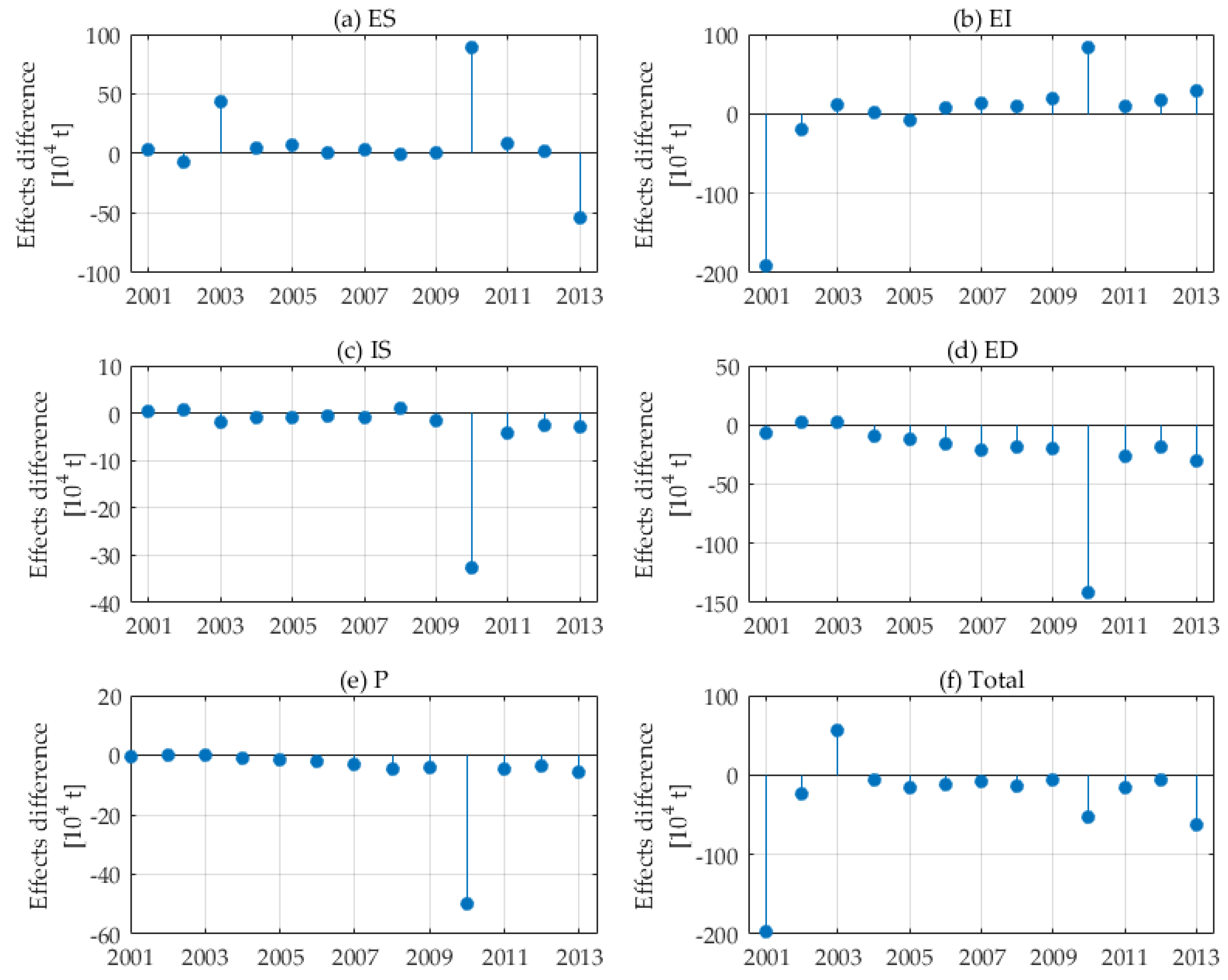
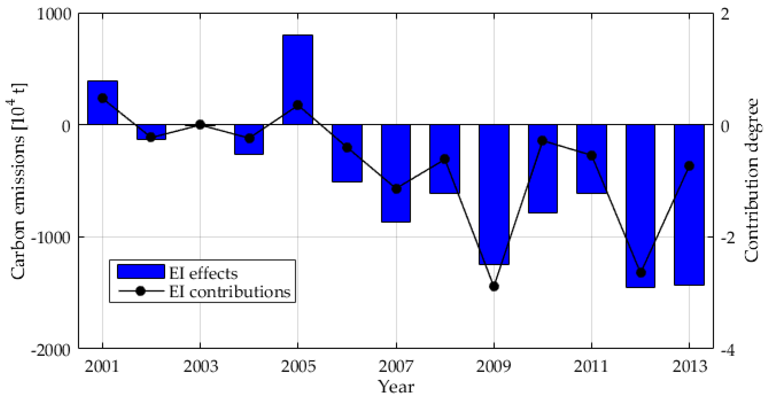
4.3. Analysis of Decomposition Results

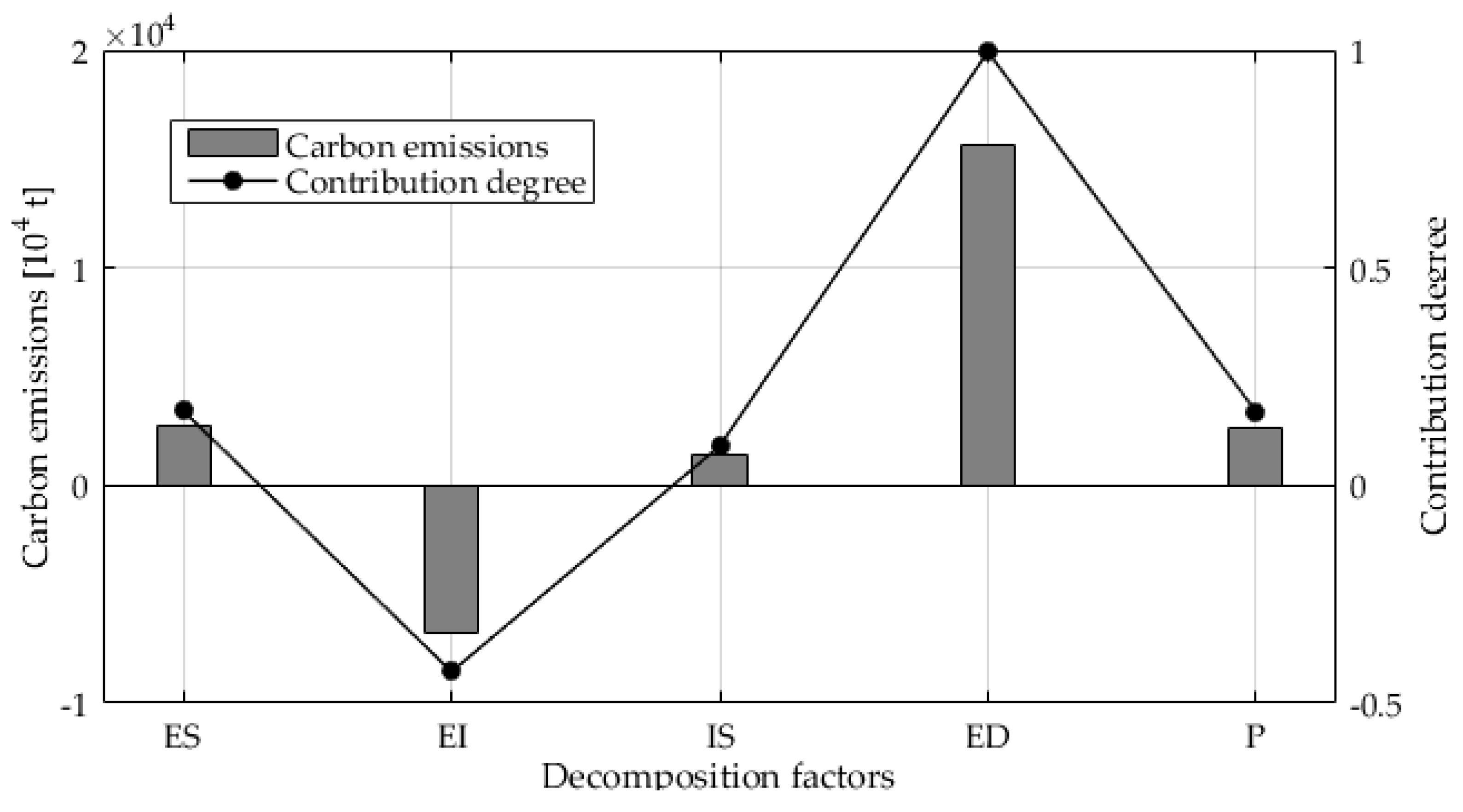
4.3.1. Cumulative Effects Analysis

As shown in Figure 4, the cumulative effect of energy consumption intensity during 2001–2013 was negative, on the contrary, the cumulative effects of energy consumption structure, industrial structure, economic development and population size were positive, reflecting that the changes of energy consumption intensity played an inhibitory effect on carbon emissions in the B-T-H region, while the changes of the energy consumption structure, industrial structure, economic development and population size played a promoting role. For the contribution degree of cumulative effects, the factor of economic development, which was the most important factor for the growth of carbon emissions of energy consumption, contributed most and was responsible for an overwhelming proportion, accounting for 99.62% of the total carbon emissions. Compared with that of the economic development, the contribution to carbon emissions of energy consumption intensity, industrial structure, population size and energy consumption structure was relatively lesser, whose contribution ratio was −42.79%, 9.06%, 16.96% and 17.15% respectively.

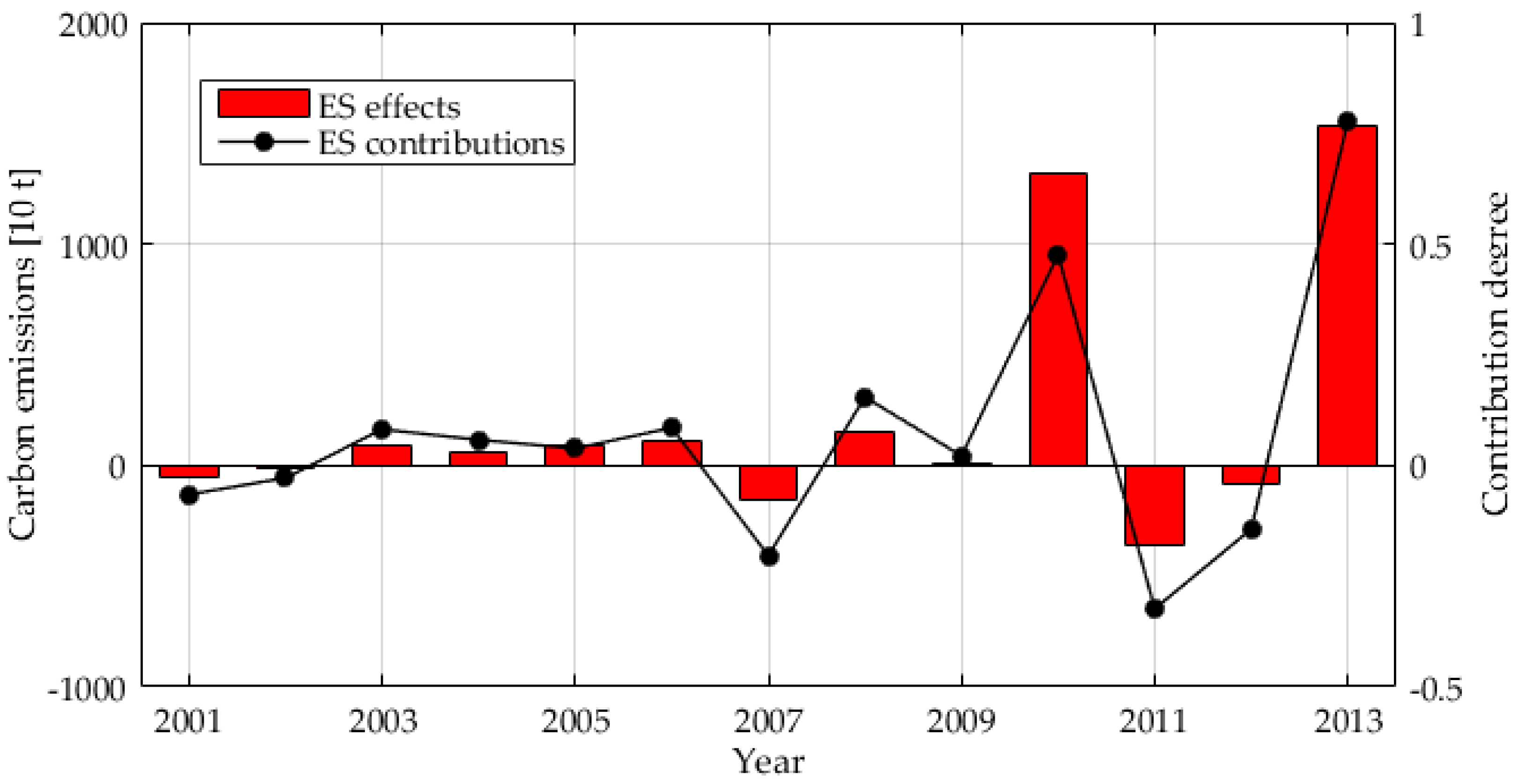
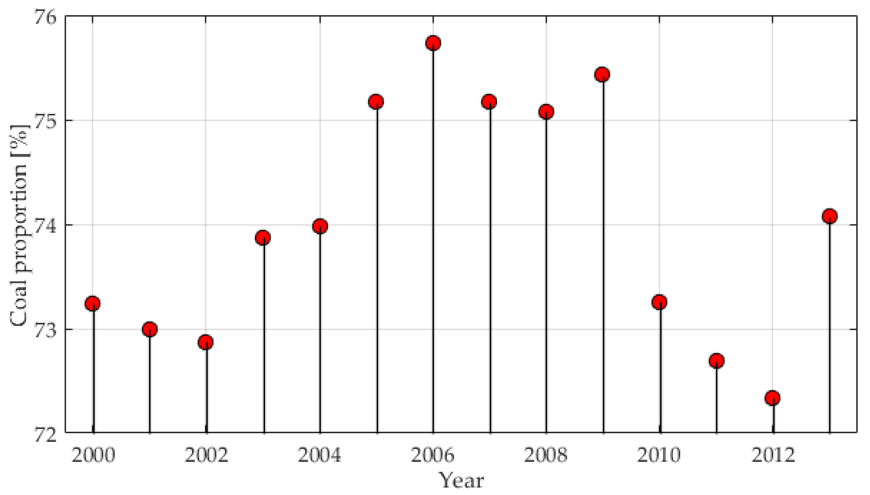
4.3.2. Analysis of Energy Consumption Structure Effects

As shown in Figure 5, the annual contribution effects of energy consumption structure fluctuated significantly, which were negative in 2001, 2002, 2007, 2011 and 2012, and were positive in other years. It was worth noting that the abnormal contribution effects in 2010 and 2013 reached 13,206.9 thousand tons and 15,359.5 thousand tons, respectively, dramatically stimulating the rapid growth of carbon emissions. The main reason is that the proportion of coal consumption has shown a downward trend in these 2 years [37,38,39]. The contribution effects in the other years were smaller, which slightly pulled the carbon emissions growth.

As shown in Figure 6, it is clear that the ratio of coal consumption to end-energy consumption in the B-T-H region in 2001, 2002, 2007, 2011 and 2012 showed a falling trend which was consistent with the trend of energy consumption structure on carbon emissions, indicating that reducing coal consumption suppressed carbon emissions growth to a certain extent; in addition, the proportion increase of oil and other fossil fuels might have led to the anomalies in 2010 and 2013 [37,38,39]. From the viewpoint of contribution degree, the absolute value of the annual contribution effects of energy consumption structure was relatively low, indicating that the energy consumption structure in the B-T-H region should be further optimized to give full pay to carbon reduction.

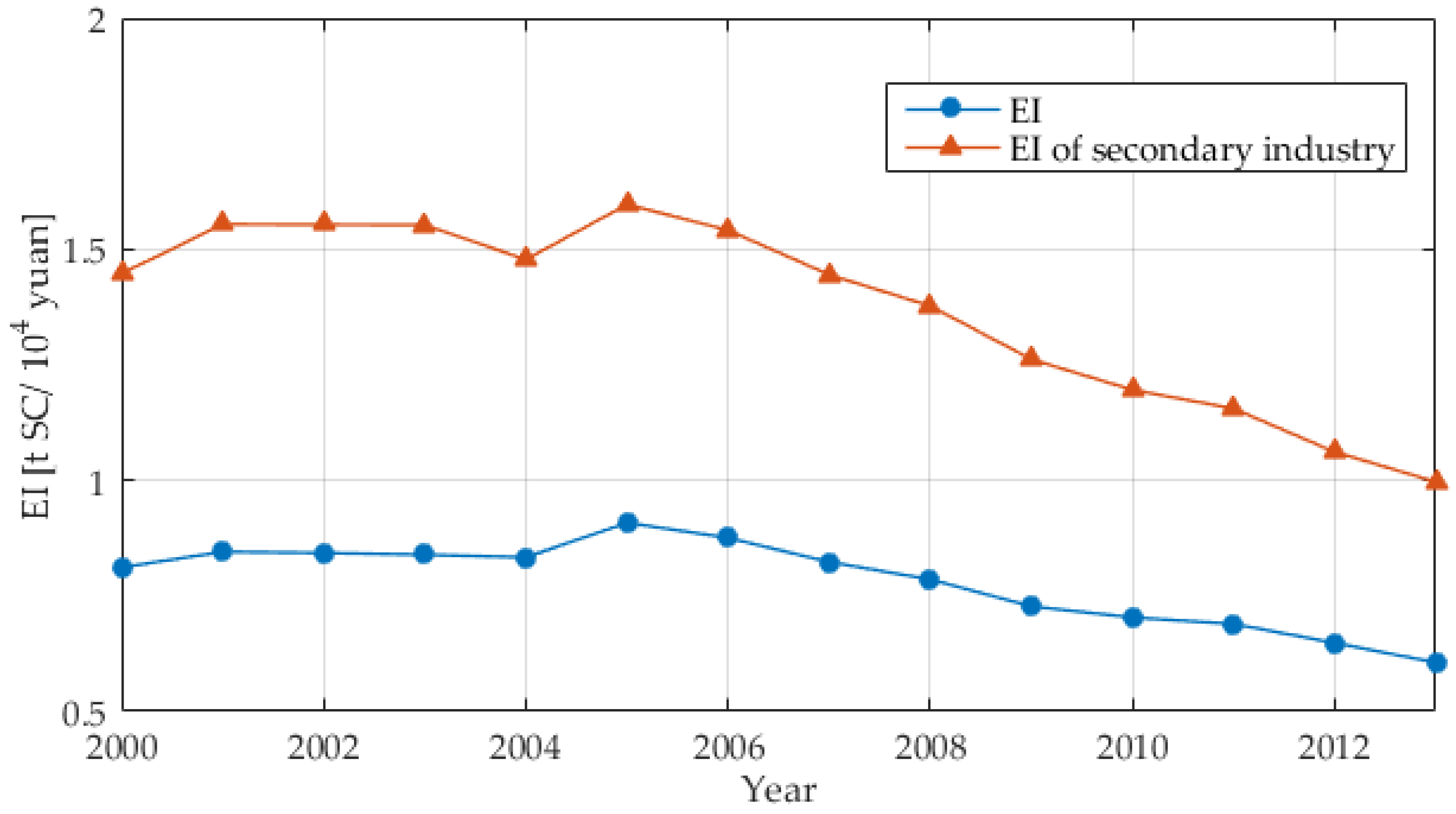
4.3.3. Analysis of Energy Consumption Intensity Effects

As shown in Figure 7, the annual contribution effects of energy consumption intensity were in a state of fluctuation. Except that the contribution effects in 2001 and 2005 were positive, in 2002–2004 and 2006–2012, the contribution effects were negative during which the average value reached −7205.3 thousand tons, indicating that energy consumption intensity had a significant inhibitory effect on carbon emissions.

The energy consumption intensity trend of the secondary industry was in accordance with the total energy consumption intensity trend in the B-T-H region, as shown in Figure 8. However, the energy consumption intensity of the secondary industry, whose changing trend was more significant, tended to descend except in 2001 and 2005. Thus, it could be concluded that the increase of energy consumption intensity of the secondary industry would promote the carbon emissions growth, and vice versa. From the view point of the contribution degree, the absolute value of contribution effects of energy consumption intensity was relatively great, which obviously inhibited the growth of carbon emissions in the B-T-H region, suggesting that, in the future, energy consumption intensity, especially that of the second industry should be cut down to effectively inhibit the carbon emissions growth.

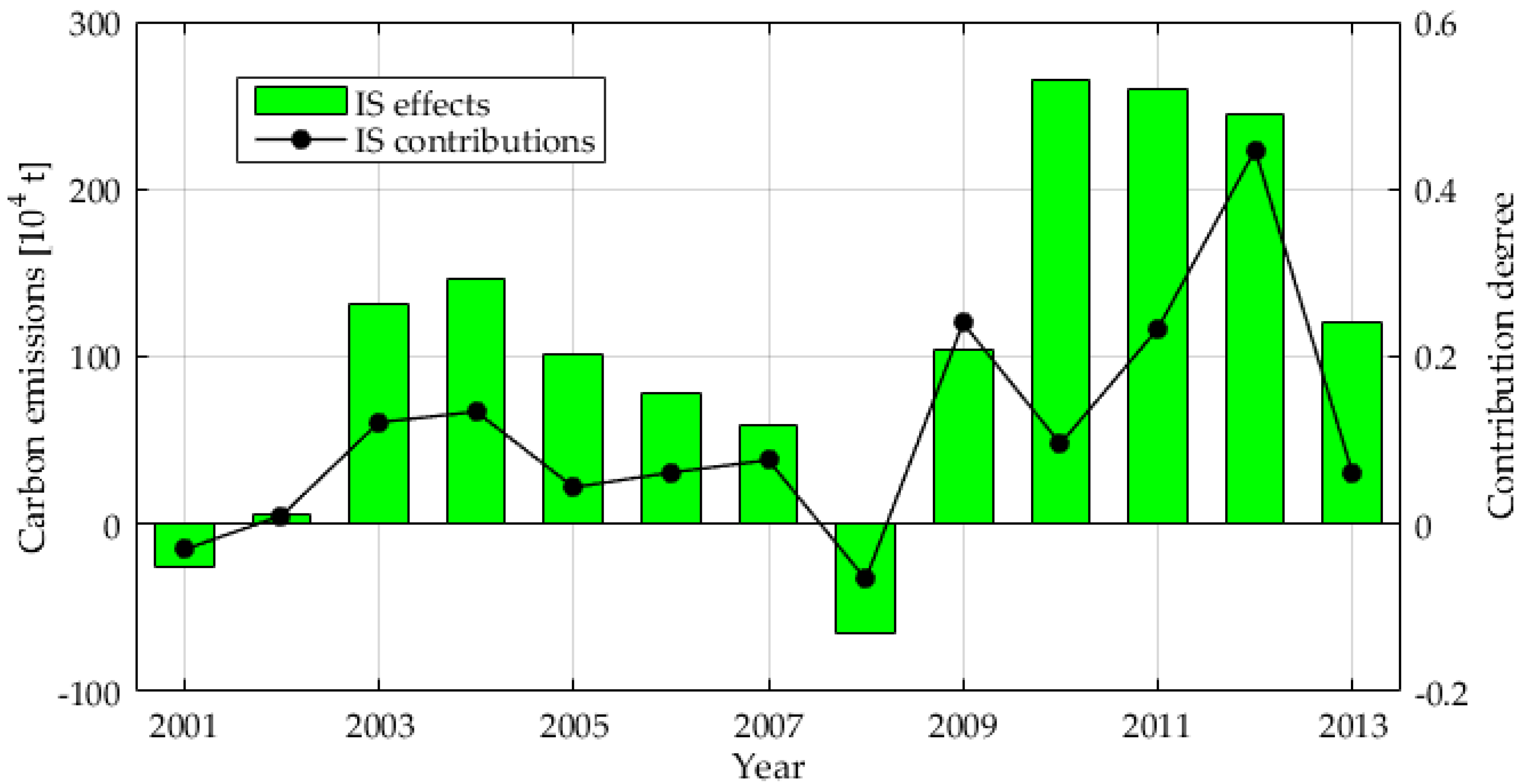
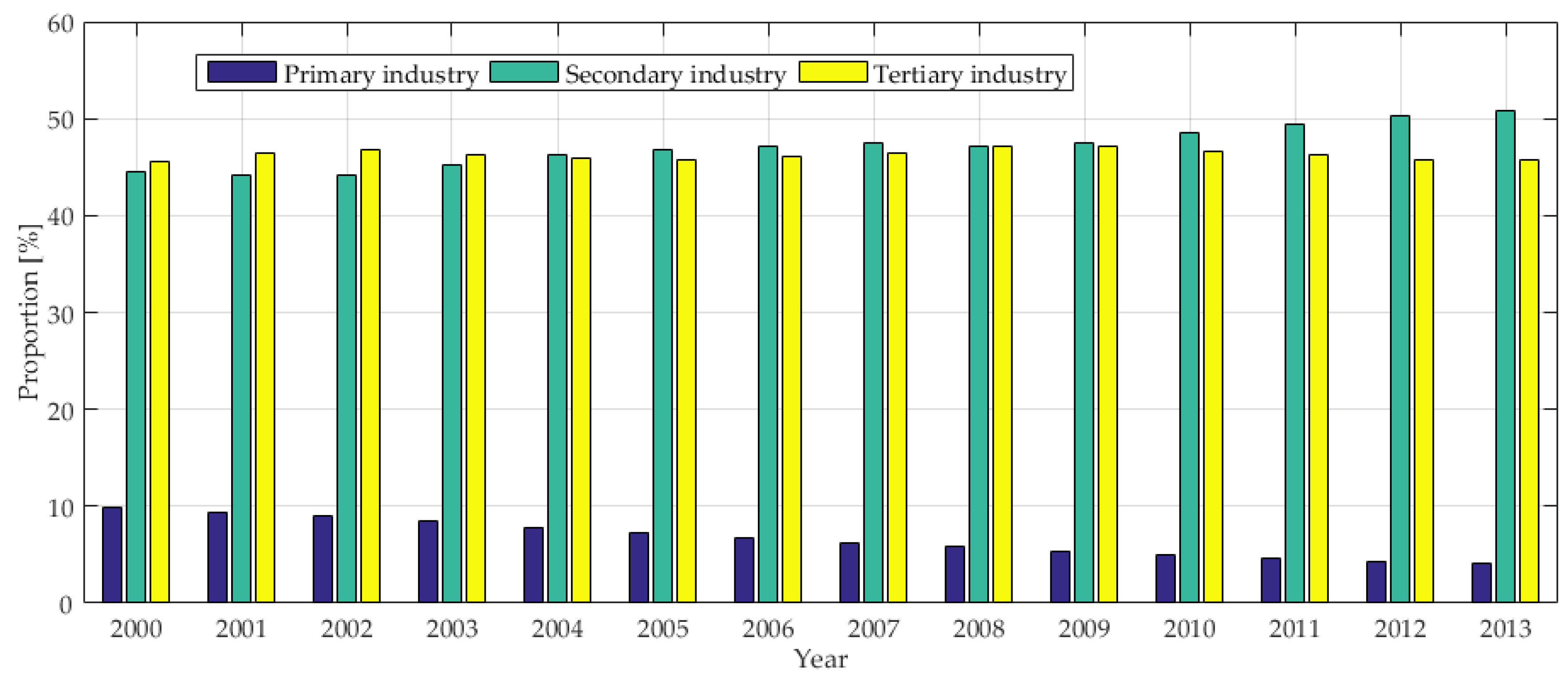
4.3.4. Analysis of Industrial Structure Effects

As shown in Figure 9, on the whole, the factor of industrial structure drove carbon emissions growth. Specifically, the study period can be divided into three stages: during 2001–2004, the contribution effects of industrial structure on carbon emissions turned from negative to positive gradually, indicating that it started to play a pulling role on carbon emissions growth; from 2005, the contribution effects decreased and finally dropped to become negative in 2008; during the period of 2009–2013 when the pulling role was weak, the contribution effects of industrial structure on carbon emissions remained at the average of 1990.2 thousand tons.

The changing trend illustrated in Figure 9 had a certain relationship with the industrial structure changes in the B-T-H region. As shown in Figure 10, during 2002–2007, the proportion of the secondary industry accounting for GDP had steadily increased, then declined slightly in 2008, from then on it climbed up continuously. Therefore, it can be concluded that the decline in GDP proportion of the second industry in the B-T-H region significantly inhibited carbon emissions growth energy. From the viewpoint of contribution degree, the absolute value of the contribution effects of industrial structure was relatively slight, suggesting that the industrial structure of the B-T-H region needed to be further improved and that rationally reducing the GDP proportion of the second industry would be a benefit in controlling carbon emissions.

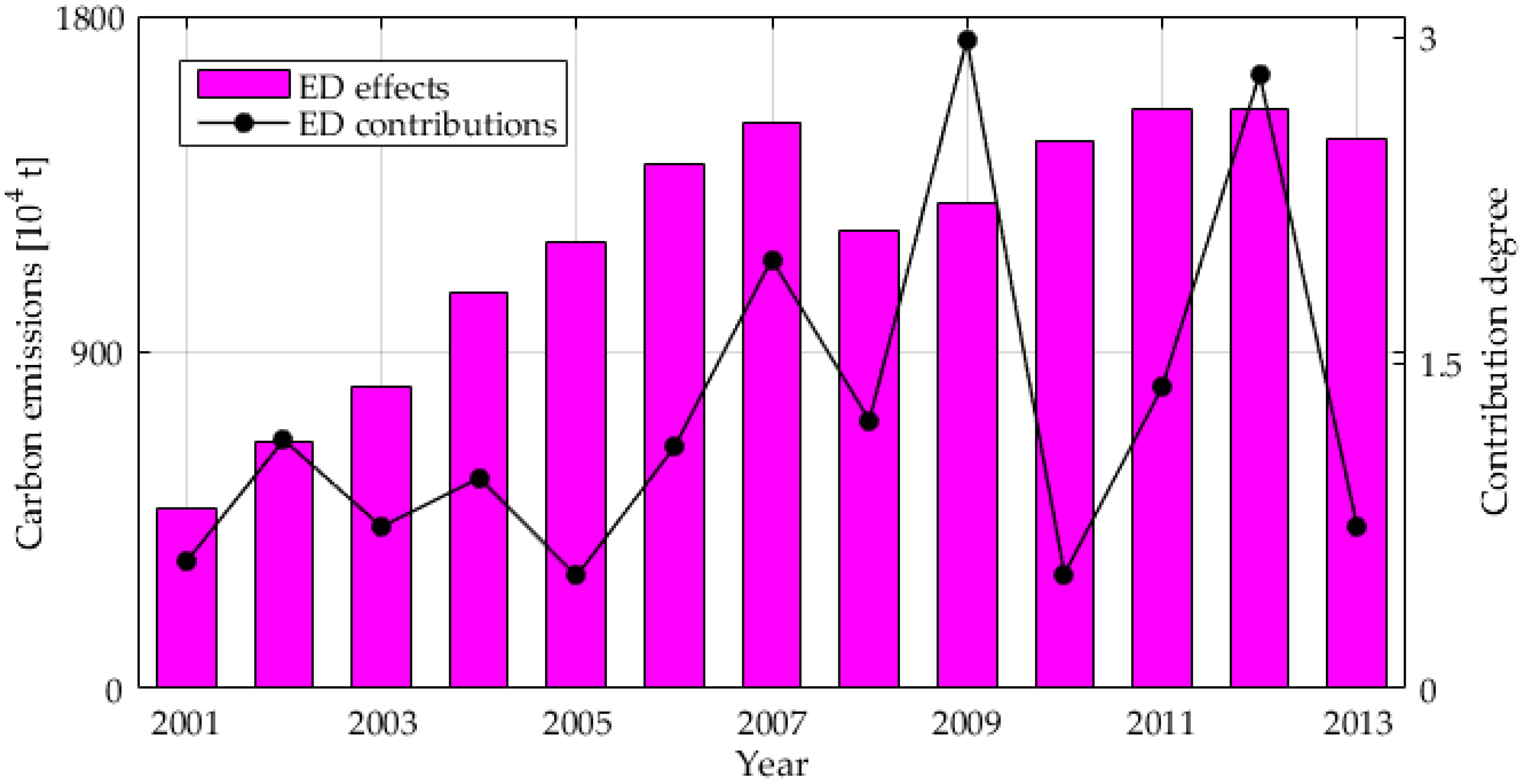
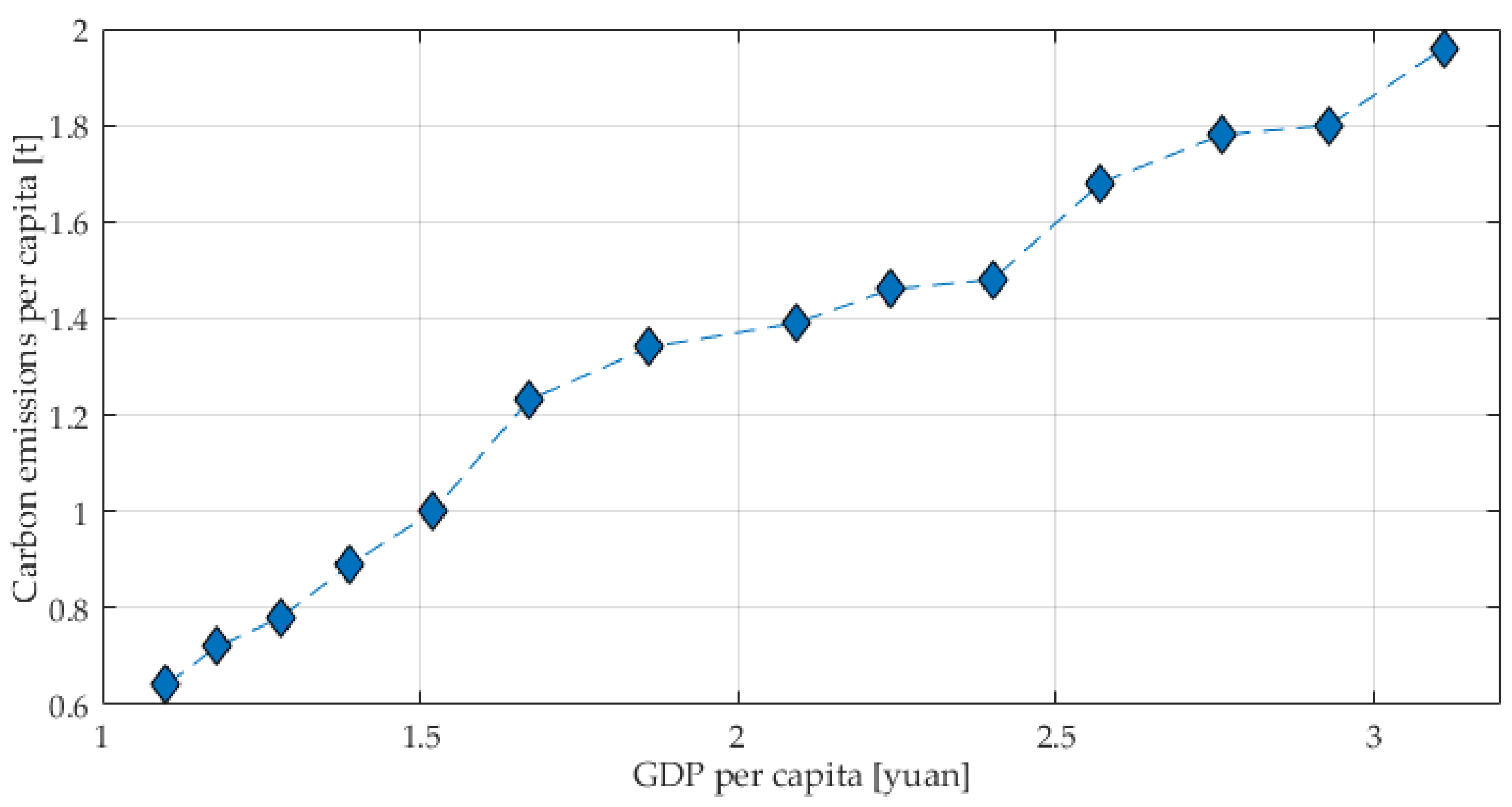
4.3.5. Analysis of Economic Development Effects

As shown in Figure 11, the effects of economic development which were all positive and huge, and the great contribution degree indicated that the economic development significantly gave impetus to carbon emissions growth of energy consumption.

From a macro point of view, China is now in the middle stage of industrial development where the rapid economic development heavily depends on energy, transport and other energy-intensive sectors who remain be the major infrastructure industry departs for a long time in the future. In the B-T-H region, especially in Hebei Province, the energy-intensive industries developed too fast, resulting in continuous carbon emissions growth. Combined with the development process of developed countries, in the process of industrialization development, economic development, carbon emissions and per capita GDP are generally supposed to experience the “inverted U” curve development. When on the left side of the curve, the region is certain and inevitable to suffer from the carbon emissions growth caused by economic development, putting the region in the dilemma of economic growth and carbon emission reduction; in contrast, when on the right side of the curve, which is in the decline phase, the region will extricate itself from the plight to realize economic growth and carbon emissions reduction.

Figure 12 clearly demonstrates that the B-T-H region was on the left side of the “inverted U” curve at the period of 2000–2013. The per capita GDP increased from 11.0 thousand yuan in 2000 to 31.1 thousand yuan in 2013. Meanwhile, the per capita carbon emissions surged from 0.64 tons in 2000 to 1.96 tons in 2013. Consequently, we can draw the conclusion that the B-T-H region is in the dilemma of economic growth and carbon emission reduction, i.e., the rapid development of the economy stimulates carbon emissions growth and it is not practical to control carbon emission by slowing economic growth down, as a result, effective ways should be explored to reduce the carbon emissions.

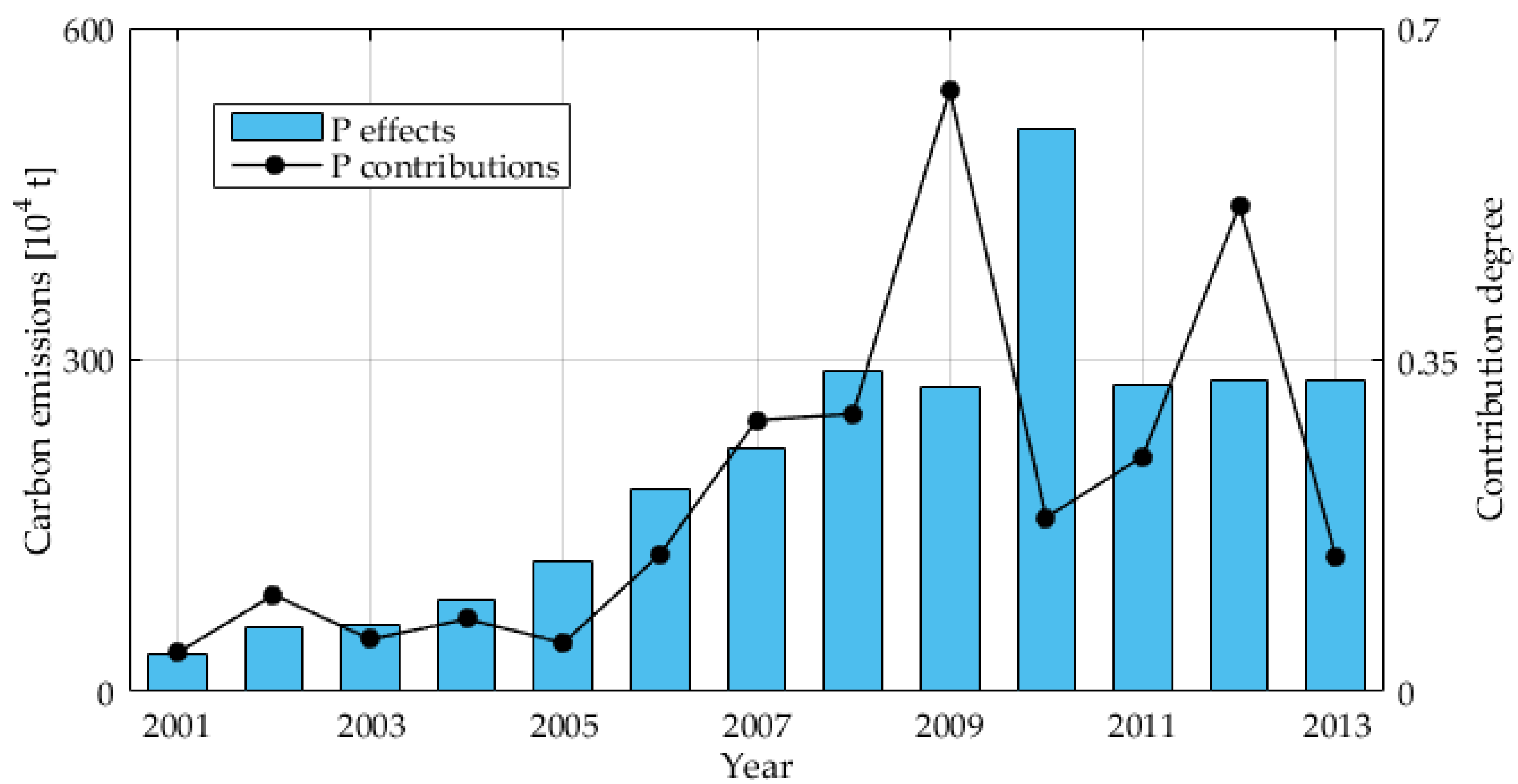
4.3.6. Analysis of Economic Population Size

Figure 13 demonstrates that the annual effects of population size on carbon emissions from 2000–2013 continued to be positive, that is to say, the population size increase led to the carbon emissions growth. Even though the growth rate of population size slowed down in recent years, the huge population base was bound to bring great population increase in volume, which led to the increase of energy demand, transportation, infrastructure and the necessities of life, thus pushing forward the consumption of fossil fuels and other energy sources to drive carbon emissions growth. In addition, the increase of population in poor areas will increase the energy demand to a great extent, which accelerates the destruction of the ecological environment and is against realizing forest carbon sequestration, thus reducing the absorption of carbon dioxide and driving carbon emissions growth [41]. The contribution of population size is relatively small with an average value of 22,054.5 thousand tons, indicating that its pulling effect was slight compared with other factors.

4.4. Suggestions

On the basis of the decomposition results and the analysis of the factors affecting carbon emissions, in this paper, we put forward the following suggestions to further control of the unreasonable carbon emissions condition in the B-T-H region.

4.4.1. Readjusting the Industrial Structure and Promoting Industrial Upgrading

According to the decomposition results, we could reach the conclusion that the proportion reduction of the second industry did benefit in controlling carbon emissions growth and cutting down carbon emission intensity. From the perspective of the industrial structure in the B-T-H region during 2000–2013, the secondary industry accounted most with the steady increasing trend, followed by the tertiary industry with fluctuations and the primary industry who accounted least with the downward trend. The differences of the industrial structure in Beijing, Tianjin and Hebei Province led to the characteristics described above: In Beijing, the tertiary industry who accounted most tended to increase, followed by the secondary industry who was falling down and the primary industry with the declining trend; Tianjin City and Hebei Province were both in economic vertical integration that the second industry accounted for an overwhelming proportion with the upward trend, followed by the tertiary industry who was decreasing and the primary industry with a downward trend. As a matter of fact, the secondary industry does contribute enormously to economic development, therefore, it is crucial to promote energy saving under the precondition of not affecting the economic development. What is most effective is to pull forward industrial upgrading, reconstruct the high energy-consuming industries, eliminate backward production productivity and optimize excessive productivity in Tianjin and Hebei areas; besides, the productivity which does not conform to the capital functions of Beijing City under the background of coordinated development for the B-T-H region should be transferred to Tianjin and Hebei as soon as possible.

4.4.2. Strengthening Technological Progress, and Constantly Reducing the Intensity of Energy Consumption

The reduction of energy consumption intensity whose contribution degree reached −49.27%, played a significant role on inhibiting carbon emissions growth and decreasing carbon emission intensity in the B-T-H region. Technological progress is the key to reducing energy consumption intensity. On the one hand, the government is supposed to insist that science and technology is the primary productive force, to provide more guidance and support to the enterprises, and to narrow the gap with the developed countries in science and technological ability; on the other hand, it is of great importance to strengthen exchanges with foreign developed countries, to introduce advanced energy technologies, shorten the time of technology progress and reduce the cost, and to promote the work of technological progress. In addition, the policy should be confirmed as the guarantee for making technical progress and reducing energy consumption intensity to vigorously launch reduction work in the B-T-H region.

4.4.3. Actively Optimizing the Energy Structure

The analysis of the energy consumption structure reflected that the coal consumption made up for a huge proportion of energy consumption in the B-T-H region, which indicated that reducing coal consumption was of significance to inhibit carbon emissions growth. Therefore, reducing the proportion of coal consumption and optimizing the structure of energy consumption should be the focus of energy saving and emission reduction work. Further, through the analysis of the three areas, Hebei Province got the first place, whose coal consumption proportion of total energy consumption ran up to over 85% in the recent 10 years without a decreasing trend, followed by the Tianjin City with the coal consumption proportion of 45%, and Beijing City whose coal consumption proportion was lowest at about 20%. Therefore, much more efforts should be made to strengthen the energy structure adjustment in Hebei Province and Tianjin City, thereby reducing the overall coal consumption ratio. According to relevant references, Hebei and Tianjin mainly used coal for power generation and heating. Thus, especially for Hebei Province and Tianjin City, the policy of clean utilization of fossil energy and development of non-fossil should always be guaranteed and shown to work. On the one hand, emphasis is supposed to be paid to strengthen the clean use of coal, improve coal utilization efficiency, and strengthen the treatment of carbon emissions; on the other hand, gradually reducing coal and oil consumption, increasing the supply of natural gas, advocating the projects of changing fuel from coal to natural gas, and further encouraging the use of clean energy such as solar energy, wind energy and biomass energy to enlarge the proportion of renewable energy consumption are all in necessity to form a multi-complementary energy consumption structure reasonably and reduce carbon emissions in the B-T-H region.

4.4.4. Building a Long-Term Carbon-Emissions-Reduction Mechanism

There is no doubt that it is of great necessity to establish a long-term mechanism of carbon emissions to carry out the work of energy-saving and emission-reduction in the B-T-H region. For one thing, the government should fully play the role of “ the visible hand” for managers, coordinate the interests of the 13 cities in the B-T-H region under the premise of high fairness and efficiency, and make timely negotiation on regional issues, thus to establish the long-term cooperation mechanism between the three governments for policy formulation and low-carbon industrial clusters establishment; meanwhile, the government performance appraisal system should be established to reduce irrational competition of excessive investment among local governments and to carry out effective assessment and accountability on government officials. For another, the advantages of “the invisible hand” of the market and market means that such as the carbon emission quota, carbon emissions trading, green finance and credit should be fully used. In particular, emphasis should be paid on the establishment of the regional carbon rights trading market, which increases the cost of carbon emissions to stimulate the implementation of carbon emission reduction.

5. Conclusions

As the third biggest economic circle in China, the B-T-H region, which is characterized by high regional production, enormous energy consumption and prominent environmental problems, is facing unprecedented pressure of carbon emission reduction. To accurately analyze the potential influencing factors affecting carbon emissions, in this paper, based on the measurement of carbon emissions in the B-T-H region by the direct carbon emissions coefficient method, the weighted-combination decomposition analysis model, who was made up by LMDI and SV, was applied to quantitatively analyze the effects on carbon emissions during 2001–2013 caused by five factors, including energy consumption structure, energy consumption intensity, industrial structure, economic development and population size. Consequently, the results were as follows: (1) The carbon emissions had shown a sustained growth trend in the B-T-H region with some differences in growth rate among the three areas. In detail, Hebei Province got the first place in carbon emissions with the annual growth rate of 12.68%, followed by Tianjin whose growth rate was 9.35%, and Beijing whose growth rate was 1.53%; (2) economic development was the main driving force for carbon emissions growth in the B-T-H region, whose cumulative contribution degree reached 99.62%. Energy consumption structure, population size and industrial structure promoted carbon emissions growth as well, but the effects weakened in turn and were less obvious than that of economic development; (3) energy consumption intensity played a significant inhibitory role on the carbon emissions growth, whose contribution degree was −42.79%. Further, there was evidence to suggest that reducing energy consumption intensity did benefit in controlling carbon emissions growth. Constrained by the limitations of the decomposition model, this paper only quantitatively analyzes the five factors affecting energy consumption carbon emissions, and factors such as technology level and government policies are not taken into account, and this will be studied in depth in the future.

References

1. Lin, B.; Tan, R. Sustainable development of China’s energy intensive industries: From the aspect of carbon dioxide emissions reduction. Renew. Sustain. Energy Rev. 2017, 77, 386–394. [Google Scholar] [CrossRef]
2. Sun, W.; Meng, M.; He, Y.; Chang, H. CO2 Emissions from China’s Power Industry: Scenarios and Policies for 13th Five-Year Plan. Energies 2016, 9, 825. [Google Scholar] [CrossRef]
3. Ma, X.; Wang, J.; Yu, F. Can MODIS AOD be employed to derive PM2.5 in Beijing-Tianjin-Hebei over China? Atmos. Res. 2016, 181, 250–256. [Google Scholar] [CrossRef]
4. Cai, S.; Wang, Y.; Zhao, B.; Wang, S.; Chang, X.; Hao, J. The impact of the “Air Pollution Prevention and Control Action Plan” on PM2.5 concentrations in Jing-Jin-Ji region during 2012–2020. Sci. Total Environ. 2017, 580, 197–209. [Google Scholar] [CrossRef] [PubMed]
5. Zhang, Y.; Zheng, H.; Yang, Z.; Li, Y.; Liu, G.; Su, M.; Yin, X. Urban energy flow processes in the Beijing-Tianjin-Hebei (Jing-Jin-Ji) urban agglomeration: Combining multi-regional input-output tables with ecological network analysis. J. Clean. Prod. 2016, 114, 243–256. [Google Scholar] [CrossRef]
6. Wang, S.; Ma, H.; Zhao, Y. Exploring the relationship between urbanization and the eco-environment—A case study of Beijing-Tianjin-Hebei region. Ecol. Indic. 2014, 45, 171–183. [Google Scholar] [CrossRef]
7. Wu, Y.; Zhao, Y. Beijing-Tianjin-Hebei Energy Consumption, Carbon Emissions and Economic Growth. Econ. Manag. 2014, 28, 5–12. [Google Scholar]
8. Feng, D.; Li, J. Research of the carbon dioxide emission efficiency and reduction potential of cities in the Beijing-Tianjin-Hebei Region. Resour. Sci. 2017, 39, 978–986. [Google Scholar]
9. Yan, Y. The Carbon Footprint’s Trends and Its Drivers in Beijing-Tianjin-Hebei Region. Soft Sci. 2016, 30, 10–14. [Google Scholar]
10. Piao, S.; Li, J. Measurement and Assessment of Carbon Reduction Capability in Beijing-Tianjin-Hebei Region. Sci. Technol. Manag. Res. 2016, 5, 193–198. [Google Scholar]
11. Cayuela, M.L.; Aguilera, E.; Sanz-Cobena, A. Direct nitrous oxide emissions in Mediterranean climate cropping systems: Emission factors based on a meta-analysis of available measurement data. Agric. Ecosyst. Environ. 2017, 238, 25–35. [Google Scholar] [CrossRef] [Green Version]
12. Lenox, C.; Kaplan, P.O. Role of natural gas in meeting an electric sector emissions reduction strategy and effects on greenhouse gas emissions. Energy Econ. 2016, 60, 460–468. [Google Scholar] [CrossRef]
13. Selvakkumaran, S.; Limmeechokchai, B.; Masui, T.; Hanaoka, T.; Matsuoka, Y. Low carbon society scenario 2050 in Thai industrial sector. Energy Convers. Manag. 2014, 85, 663–674. [Google Scholar] [CrossRef]
14. Yang, L.; Cai, Y.; Zhong, X. A Carbon Emission Evaluation for an Integrated Logistics System—A Case Study of the Port of Shenzhen. Sustainability 2017, 9, 462. [Google Scholar] [CrossRef]
15. IPCC. 2006 IPCC Guidelines for National Greenhouse Gas Inventories; IGES: Ibaraki Prefecture, Japan, 2006. [Google Scholar]
16. International Organization for Standardization. Available online: https://www.iso.org/standard/38381.html (accessed on 31 May 2018).[Green Version]
17. World Resources Institute, World Business Council on Sustainable Development. Available online: http://www.ghgprotocol.org/ (accessed on 31 May 2018).
18. British Standards Institution. Available online: https://www.bsigroup.com/en-GB/PAS-2060-Carbon-Neutrality/ (accessed on 31 May 2018).
19. Nag, B.; Parikh, J.K. Carbon emission coefficient of power consumption in India: Baseline determination from the demand side. Energy Policy 2005, 33, 777–786. [Google Scholar] [CrossRef]
20. Wang, C.; Wang, F.; Zhang, X.; Zhang, H. Influencing mechanism of energy-related carbon emissions in Xinjiang based on the input-output and structural decomposition analysis. J. Geogr. Sci. 2017, 27, 365–384. [Google Scholar] [CrossRef]
21. Nie, H.; Kemp, R.; Vivanco, D.F.; Vasseur, V. Structural decomposition analysis of energy-related CO2 emissions in China from 1997 to 2010. Energy Effic. 2016, 9, 1351–1367. [Google Scholar] [CrossRef]
22. Sun, W.; He, Y.; Chang, H. Regional characteristics of CO2 emissions from China’s power generation: Affinity propagation and refined Laspeyres decomposition. Int. J. Glob. Warm. 2017, 11, 38–66. [Google Scholar] [CrossRef]
23. Zhang, X.; Zhao, Y.; Sun, Q.; Wang, C. Decomposition and Attribution Analysis of Industrial Carbon Intensity Changes in Xinjiang, China. Sustainability 2017, 9, 459. [Google Scholar] [CrossRef]
24. Ang, B.W. Decomposition analysis for policymaking in energy: Which is the preferred method? Energy Policy 2004, 32, 1131–1139. [Google Scholar] [CrossRef]
25. Song, J.; Song, Q.; Zhang, D.; Lu, Y.; Luan, L. Study on Influencing Factors of Carbon Emissions from Energy Consumption of Shandong Province of China from 1995 to 2012. Sci. World J. 2014. [Google Scholar] [CrossRef] [PubMed]
26. Shorrocks, A.F. Decomposition procedures for distributional analysis: A unified framework based on the Shapley value. J. Econ. Inequal. 2013, 11, 99–126. [Google Scholar] [CrossRef]
27. Ang, B.W. The LMDI approach to decomposition analysis: A practical guide. Energy Policy 2005, 33, 867–871. [Google Scholar] [CrossRef]
28. Ang, B.W. LMDI decomposition approach: A guide for implementation. Energy Policy 2015, 86, 233–238. [Google Scholar] [CrossRef]
29. Ang, B.W.; Huang, H.C.; Mu, A.R. Properties and linkages of some index decomposition analysis methods. Energy Policy 2009, 37, 4624–4632. [Google Scholar] [CrossRef]
30. Yu, S.; Wei, Y.; Wang, K. Provincial allocation of carbon emission reduction targets in China: An approach based on improved fuzzy cluster and Shapley value decomposition. Energy Policy 2014, 66, 630–644. [Google Scholar] [CrossRef]
31. Department of Energy Statistics, National Bureau of Statistic, People’s Republic of China. China Energy Statistical Yearbook; China Statistics Press: Beijing, China, 2014.
32. Song, R.; Yang, S.; Sun, M. GHG Protocol Tool for Energy Consumption in China (Version 2.0); World Resources Institute: Washington, DC, USA, 2012. [Google Scholar]
33. National Development and Reform Commission of China. Guidelines for the Preparation of Provincial Greenhouse Gas Inventories; National Development and Reform Commission of China: Beijing, China, 2011. [Google Scholar]
34. Field, A.P. Kendall’s Coefficient of Concordance. In Encyclopedia of Statistics in Behavioral Science; John Wiley & Sons, Ltd.: Hoboken, NJ, USA, 2005. [Google Scholar]
35. Ang, B.W.; Liu, N. Handling zero values in the logarithmic mean Divisia index decomposition approach. Energy Policy 2007, 35, 238–246. [Google Scholar] [CrossRef]
36. Ang, B.W.; Liu, N. Negative-value problems of the logarithmic mean Divisia index decomposition approach. Energy Policy 2007, 35, 739–742. [Google Scholar] [CrossRef]
37. Beijing Municipal Bureau of Statistics, NBS Survey Office in Beijing. Beijing Statistical Yearbook; China Statistics Press: Beijing, China, 2014.
38. Tianjin Municipal Bureau of Statistics, NBS Survey Office in Tianjin. Tianjin Statistical Yearbook; China Statistics Press: Beijing, China, 2014.
39. The People’s Government of Hebei Province. Hebei Economic Yearbook; China Statistics Press: Beijing, China, 2014.
40. National Bureau of Statistics of China. China Statistical Yearbook; China Statistics Press: Beijing, China, 2014.
41. Liang, Y.; Fan, J.; Sun, W.; Han, X.; Ma, H.; Sheng, K.; Xu, Y.; Wang, C. The Influencing Factors of Rural Household Energy Consumption Structure in Mountainous Areas of Southwest China: A Case Study of Zhaotong City of Yunnan Province. Acta Geogr. Sin. 2012, 67, 221–229. [Google Scholar]
Figure 1. The carbon emissions in the B-T-H region.
Sustainability 10 02535 g001
Figure 2. The total carbon emissions in the B-T-H region.
Sustainability 10 02535 g002
Figure 3. The difference between the LMDI and SV.
Sustainability 10 02535 g003
Figure 4. The cumulative effects and contribution degree of 6 factors.
Sustainability 10 02535 g004
Figure 5. The effects and contribution degree of energy consumption structure.
Sustainability 10 02535 g005
Figure 6. The proportion of coal consumption to end-energy consumption.
Sustainability 10 02535 g006
Figure 7. The effects and contribution degree of energy consumption intensity.
Sustainability 10 02535 g007
Figure 8. The energy consumption intensity of B-T-H region.
Sustainability 10 02535 g008
Figure 9. The effects and contribution degree of industrial structure.
Sustainability 10 02535 g009
Figure 10. The industrial structure of B-T-H region.
Sustainability 10 02535 g010
Figure 11. The effects and contribution degree of economic development.
Sustainability 10 02535 g011
Figure 12. The per capita GDP and per capita carbon emissions curve in B-T-H region.
Sustainability 10 02535 g012
Figure 13. The effects and contribution degree of population size.
Sustainability 10 02535 g013