An Efficient Grid-Based K-Prototypes Algorithm for Sustainable Decision-Making on Spatial Objects


Abstract
1. Introduction
- We proposed an effective grid-based k-prototypes algorithm; GK-prototypes, which improves the performance of a basic k-prototypes algorithm.
- We developed a pruning technique which utilizes the minimum and maximum distance on numeric attributes and the maximum distance on categorical attributes between a cell and a cluster center.
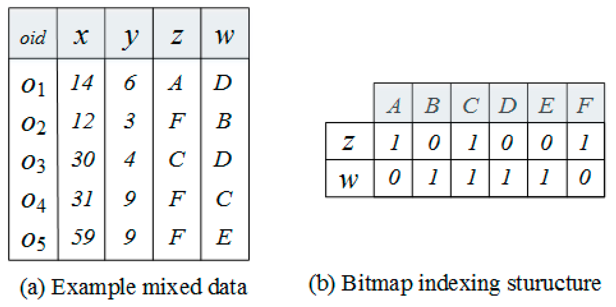
- We developed a pruning technique based on a bitmap index to improve the efficiency of the pruning in case the categorical data is skewed.
- We provided several experimental results using real datasets and various synthetic datasets. The experimental results showed that our proposed algorithms achieve better performance than existing pruning techniques in the k-prototypes algorithm.
2. Related Works
2.1. Spatial Data Mining
2.2. Clustering for Mixed Data
2.3. Grid-Based Clustering Algorithm
2.4. Existing Pruning Technique in the K-Prototypes Algorithm
3. Preliminary
4. GK-Prototypes Algorithm
4.1. Cell Pruning Technique
| Algorithm 1 The k-prototypes algorithm with cell pruning (KCP) |
| Input: k: the number of cluster, G: the grid in which all objects are stored per cell |
| Output: k cluster centers |
| 1: C[ ]← Ø // k cluster centers |
| 2: Randomly choosing k object, and assigning it to C. |
| 3: while IsConverged() do |
| 4: for each cell g in G |
| 5: dmin[ ], dmax[ ] ← Calc(g, C) |
| 6: dminmax ← min(dmax[ ]) |
| 7: candidate ← Ø |
| 8: for j ←1 to k do |
| 9: if (dminmax + mc > dmin[j] ) // Lemma 1 |
| 10: candidate ← candidate ∪ j |
| 11: end for |
| 12: min_distance ← ∞ |
| 13: min_cluster ← null |
| 14: for each object o in g |
| 15: for each center c in candidate |
| 16: if min_distance > d(o, c) |
| 17: min_cluster ← index of c |
| 18: end for |
| 19: Assign(o, min_cluster) |
| 20: UpdateCenter(C[c]) |
| 21: end for |
| 22: end while |
| 23: return C[k] |
4.2. Bitmap Pruning Technique
| Algorithm 2 The k-prototypes algorithm with bitmap pruning (KBP) |
| Input: k: the number of cluster, G: the grid in which all objects are stored per cell |
| Output: k cluster centers |
| 1: C[ ]← Ø // k cluster center |
| 2: Randomly choosing k object, and assigning it to C. |
| 3: while IsConverged() do |
| 4: for each cell g in G |
| 5: dmin[ ], dmax[ ] ← Calc(g, C) |
| 6: dminmax ← min(dmax[ ]) |
| 7: arrayContain[] ← IsContain(g, C) |
| 8: candidate ← Ø |
| 9: for j ←1 to k do |
| 10: if (dminmax + mc > dmin[j] ) // Lemma 1 |
| 11: candidate ← candidate ∪ j |
| 12: end for |
| 13: min_distance ← ∞ |
| 14: min_cluster ← null |
| 15: distance ← null |
| 16: for each object o in g |
| 17: for each center c in candidate |
| 18: if (arrayContain [c] == 0) |
| 19: distance = dr(o, c) + mc |
| 20: else |
| 21: distance = dr(o, c) + dc(o, c) |
| 22: if min_distance > distance |
| 23: min_cluster ← index of cluster center |
| 24: end for |
| 25: Assign(o, min_cluster) |
| 26: UpdateCenter(C) |
| 27: end for |
| 28: end while |
| 29: return C[k] |
4.3. Complexity
5. Experiments
5.1. Data Sets
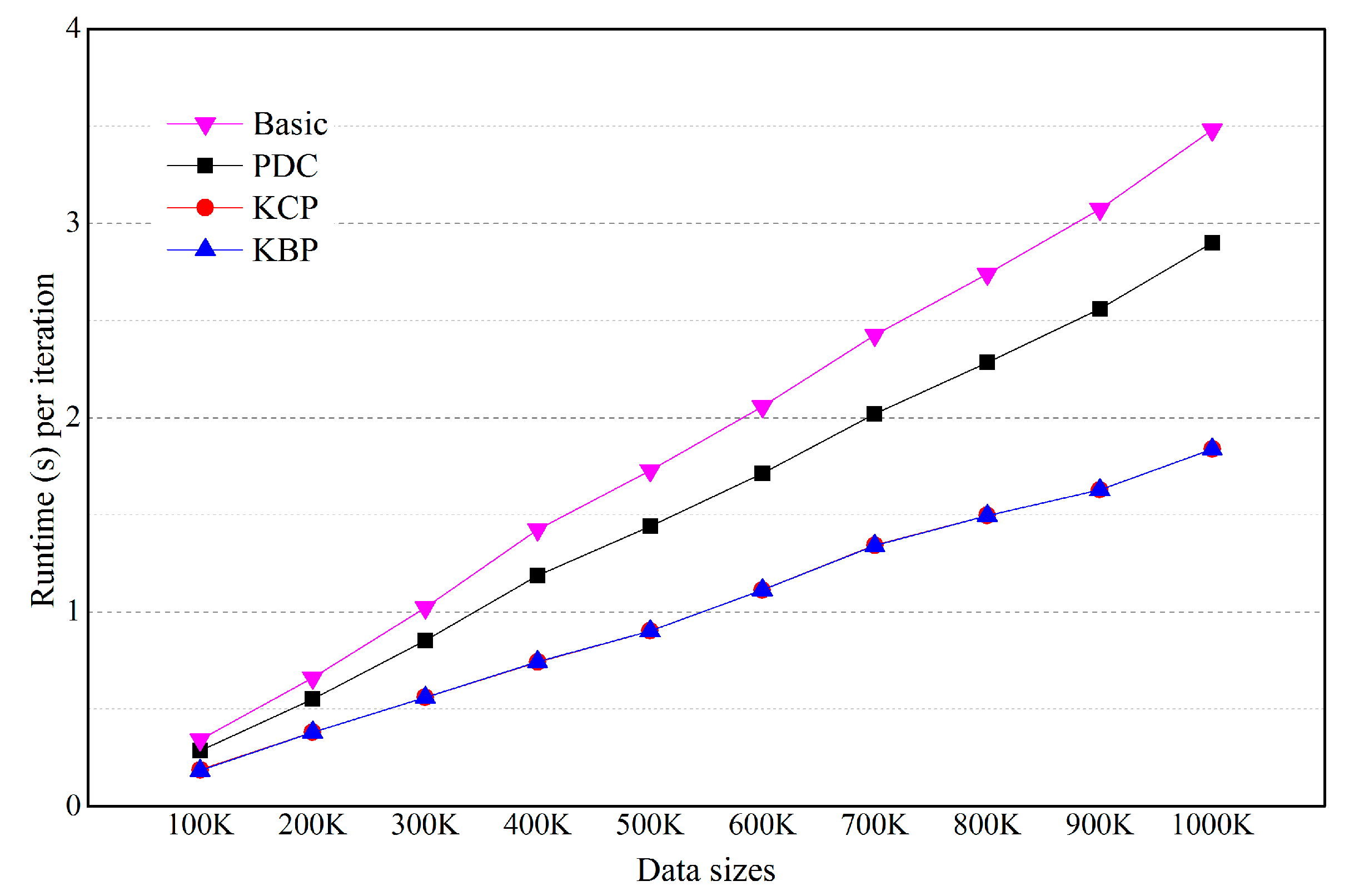
5.2. Effects of the Number of Objects
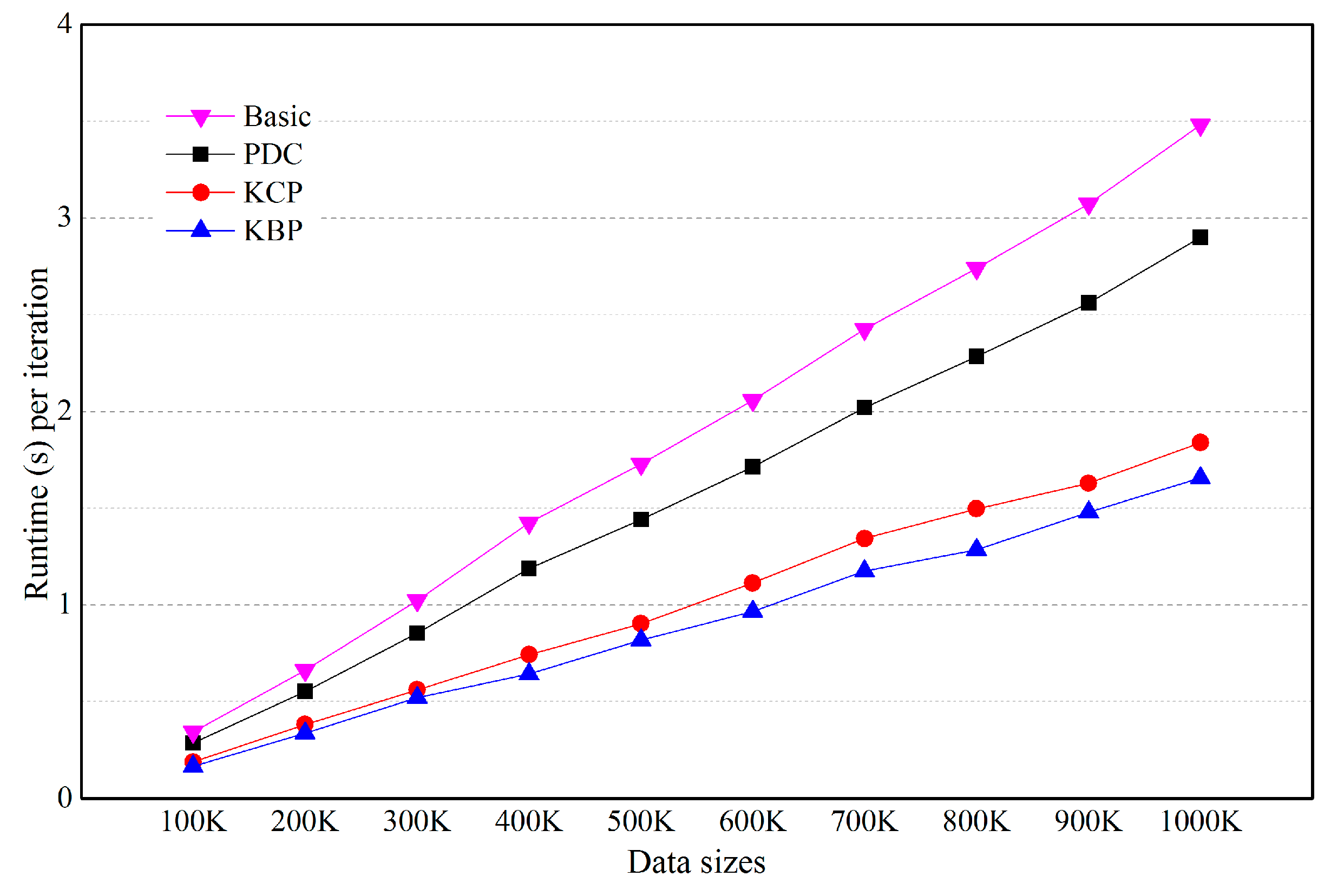
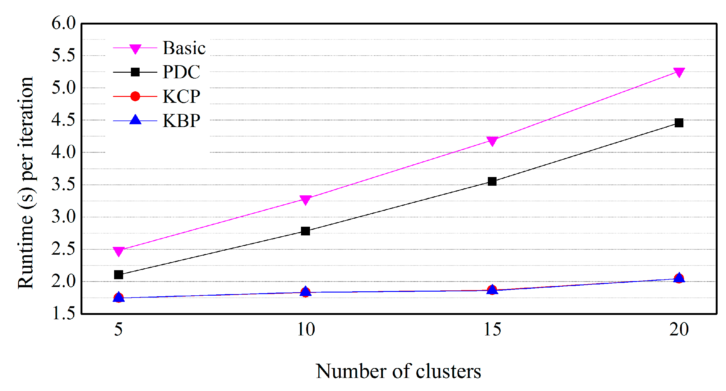
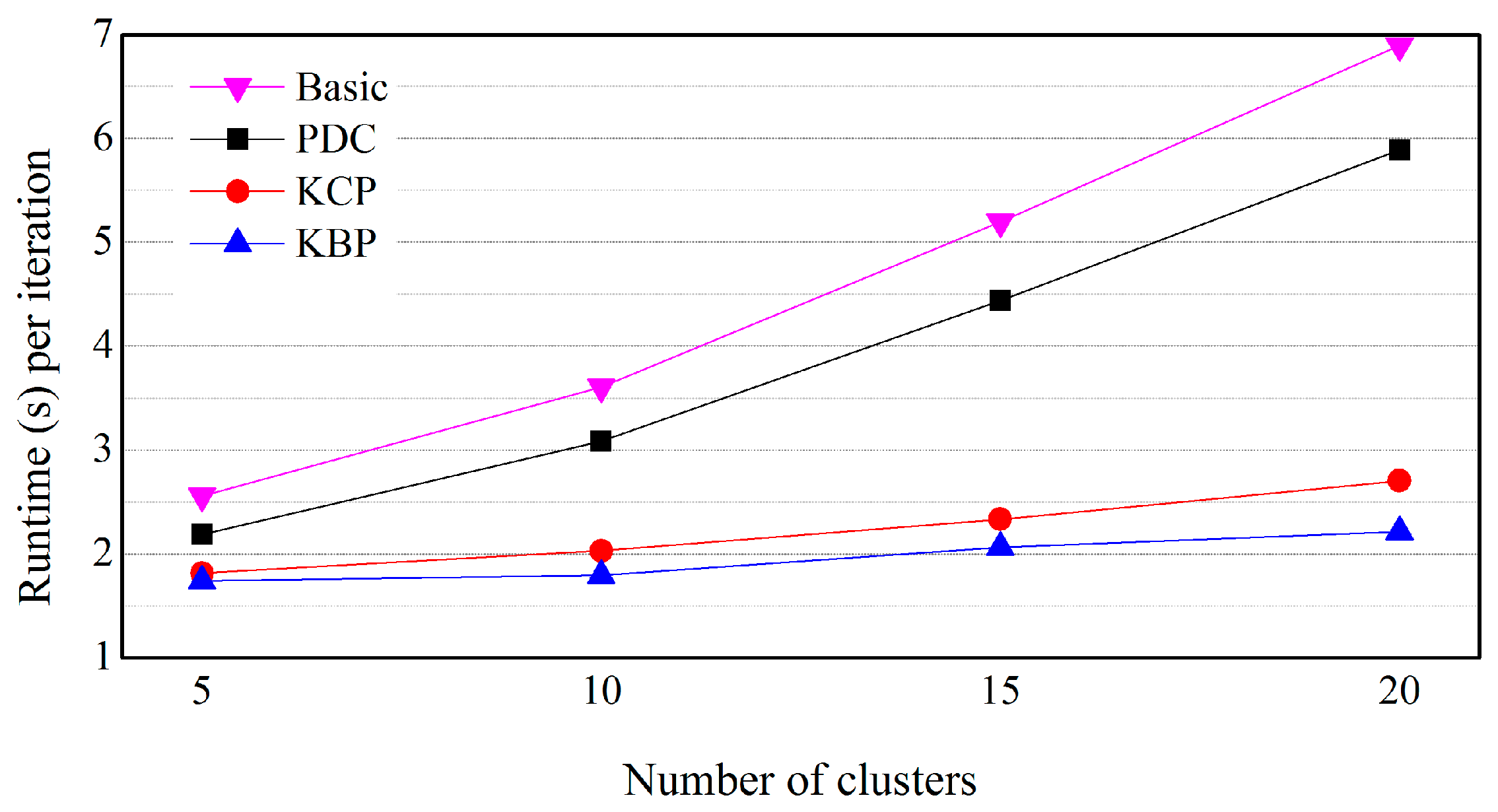
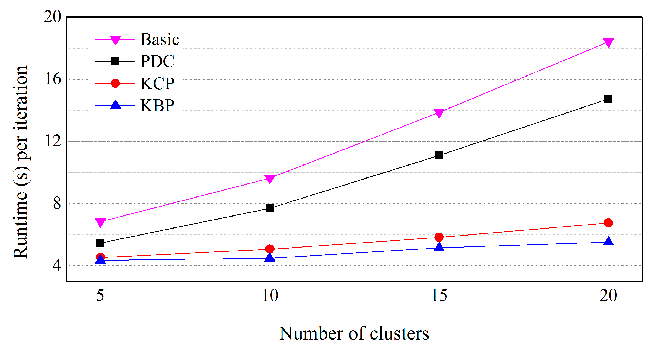
5.3. Effects of the Number of Clusters
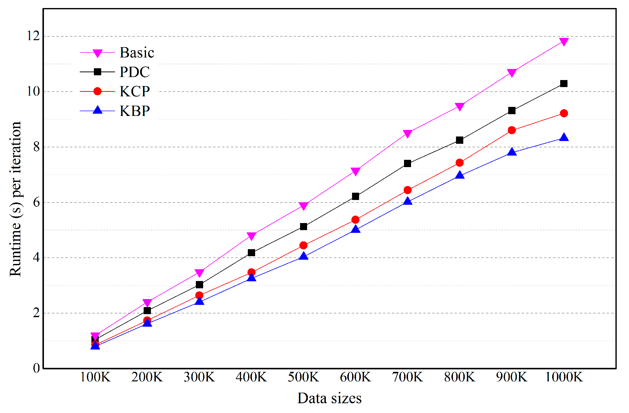
5.4. Effects of the Number of Categorical Attributes
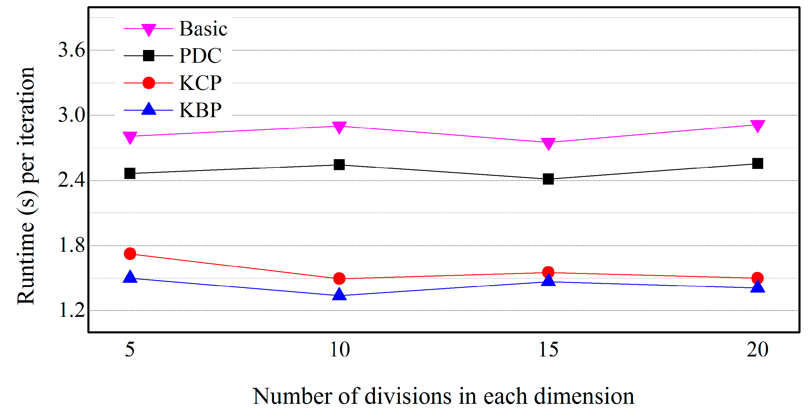
5.5. Effects of the Size of Cells
6. Conclusions
Author Contributions
Funding
Conflicts of Interest
References
- Zavadskas, E.K.; Antucheviciene, J.; Vilutiene, T.; Adeli, H. Sustainable Decision Making in Civil Engineering, Construction and Building Technology. Sustainability 2018, 10, 14. [Google Scholar] [CrossRef]
- Hersh, M.A. Sustainable Decision Making: The Role of Decision Support systems. IEEE Trans. Syst. Man Cybern. C Appl. Rev. 1999, 29, 395–408. [Google Scholar] [CrossRef]
- Gomes, C.P. Computational Sustainability: Computational Methods for a Sustainable Environment, Economy, and Society. Bridge Natl. Acad. Eng. 2009, 39, 8. [Google Scholar]
- Morik, K.; Bhaduri, K.; Kargupta, H. Introduction to Data Mining for Sustainability. Data Min. Knowl. Discov. 2012, 24, 311–324. [Google Scholar] [CrossRef]
- Aissi, S.; Gouider, M.S.; Sboui, T.; Said, L.B. A Spatial Data Warehouse Recommendation Approach: Conceptual Framework and Experimental Evaluation. Hum.-Centric Comput. Inf. Sci. 2015, 5, 30. [Google Scholar] [CrossRef]
- Kim, J.-J. Spatio-temporal Sensor Data Processing Techniques. J. Inf. Process. Syst. 2017, 13, 1259–1276. [Google Scholar] [CrossRef]
- Sander, J.; Ester, M.; Kriegel, H.P.; Xu, X. Density-Based Clustering in Spatial Databases: The Algorithm GDBSCAN and Its Applications. Data Min. Knowl. Discov. 1998, 2, 169–194. [Google Scholar] [CrossRef]
- Koperski, K.; Han, J.; Stefanovic, N. An Efficient Two-Step Method for Classification of Spatial Data. In Proceedings of the International Symposium on Spatial Data Handling (SDH’98), Vancouver, BC, Canada, 12–15 July 1998; pp. 45–54. [Google Scholar]
- Koperski, K.; Han, J. Discovery of Spatial Association Rules in Geographic Information Databases. In Proceedings of the 4th International Symposium on Advances in Spatial Databases (SSD’95), Portland, ME, USA, 6–9 July 1995; pp. 47–66. [Google Scholar]
- Ester, M.; Frommelt, A.; Kriegel, H.P.; Sander, J. Algorithms for Characterization and Trend Detection in Spatial Databases. In Proceedings of the Fourth International Conference on Knowledge Discovery and Data Mining (KDD’98), 27–31 August 1995; pp. 44–50. [Google Scholar]
- Deren, L.; Shuliang, W.; Wenzhong, S.; Xinzhou, W. On Spatial Data Mining and Knowledge Discovery. Geomat. Inf. Sci. Wuhan Univ. 2001, 26, 491–499. [Google Scholar]
- Boldt, M.; Borg, A. A Statistical Method for Detecting Significant Temporal Hotspots using LISA Statistics. In Proceedings of the Intelligence and Security Informatics Conference (EISIC), Athens, Greece, 27–31 September 2017. [Google Scholar]
- Yu, Y.-T.; Lin, G.-H.; Jiang, I.H.-R.; Chiang, C. Machine-Learning-Based Hotspot Detection using Topological Classification and Critical Feature Extraction. In Proceedings of the 50th Annual Design Automation Conference, Austin, TX, USA, 29 May–7 June 2013; pp. 460–470. [Google Scholar]
- Murray, A.; McGuffog, I.; Western, J.; Mullins, P. Exploratory Spatial Data Analysis Techniques for Examining Urban Crime. Br. J. Criminol. 2001, 41, 309–329. [Google Scholar] [CrossRef]
- Chainey, S.; Tompson, L.; Uhlig, S. The Utility of Hotspot Mapping for Predicting Spatial Patterns of Crime. Secur. J. 2008, 21, 4–28. [Google Scholar] [CrossRef]
- Di Martino, F.; Sessa, S. The Extended Fuzzy C-means Algorithm for Hotspots in Spatio-temporal GIS. Expert. Syst. Appl. 2011, 38, 11829–11836. [Google Scholar] [CrossRef]
- Di Martino, F.; Sessa, S.; Barillari, U.E.S.; Barillari, M.R. Spatio-temporal Hotspots and Application on a Disease Analysis Case via GIS. Soft Comput. 2014, 18, 2377–2384. [Google Scholar] [CrossRef]
- Mullner, R.M.; Chung, K.; Croke, K.G.; Mensah, E.K. Geographic Information Systems in Public Health and Medicine. J. Med. Syst. 2004, 28, 215–221. [Google Scholar] [CrossRef] [PubMed]
- Polat, K. Application of Attribute Weighting Method Based on Clustering Centers to Discrimination of linearly Non-separable Medical Datasets. J. Med. Syst. 2012, 36, 2657–2673. [Google Scholar] [CrossRef] [PubMed]
- Wei, C.K.; Su, S.; Yang, M.C. Application of Data Mining on the Development of a Disease Distribution Map of Screened Community Residents of Taipei County in Taiwan. J. Med. Syst. 2012, 36, 2021–2027. [Google Scholar] [CrossRef] [PubMed]
- Huang, Z. Clustering Large Data Sets with Mixed Numeric and Categorical Values. In Proceedings of the First Pacific Asia Knowledge Discovery and Data Mining Conference, Singapore, 22–24 July 1997; pp. 21–34. [Google Scholar]
- Kim, B. A Fast K-prototypes Algorithm using Partial Distance Computation. Symmetry 2017, 9, 58. [Google Scholar] [CrossRef]
- Goodchild, M. Geographical Information Science. Int. J. Geogr. Inf. Sci. 1992, 6, 31–45. [Google Scholar] [CrossRef]
- Fischer, M.M. Computational Neural Networks: A New Paradigm for Spatial Nalysis. Environ. Plan. A 1998, 30, 1873–1891. [Google Scholar] [CrossRef]
- Yao, X.; Thill, J.-C. Neurofuzzy Modeling of Context–contingent Proximity Relations. Geogr. Anal. 2007, 39, 169–194. [Google Scholar] [CrossRef]
- Frank, R.; Ester, M.; Knobbe, A. A Multi-relational Approach to Spatial Classification. In Proceedings of the 15th ACM SIGKDD International Conference on Knowledge Discovery and Data Mining, 28 June–1 July 2009; pp. 309–318. [Google Scholar]
- Mennis, J.; Liu, J.W. Mining Association Rules in Spatio-temporal Data: An Analysis of Urban Socioeconomic and Land Cover Change. Trans. GIS 2005, 9, 5–17. [Google Scholar] [CrossRef]
- Shekhar, S.; Huang, Y. Discovering Spatial Co-location Patterns: A Summary of Results. In Advances in Spatial and Temporal Databases (SSTD 2001); Jensen, C.S., Schneider, M., Seeger, B., Tsotras, V.J., Eds.; Springer: Berlin/Heidelberg, Germany, 2001. [Google Scholar]
- Wan, Y.; Zhou, J. KNFCOM-T: A K-nearest Features-based Co-location Pattern Mining Algorithm for Large Spatial Data Sets by Using T-trees. Int. J. Bus. Intell. Data Min. 2009, 3, 375–389. [Google Scholar] [CrossRef]
- Yu, W. Spatial Co-location Pattern Mining for Location-based Services in Road Networks. Expert. Syst. Appl. 2016, 46, 324–335. [Google Scholar] [CrossRef]
- Hartigan, J.A.; Wong, M.A. Algorithm as 136: A K-means Clustering Algorithm. J. R. Stat. Soc. 1979, 28, 100–108. [Google Scholar] [CrossRef]
- Sharma(sachdeva), R.; Alam, A.M.; Rani, A. K-Means Clustering in Spatial Data Mining using Weka Interface. In Proceedings of the International Conference on Advances in Communication and Computing Technologies, Chennai, India, 3–5 August 2012; pp. 26–30. Available online: https://www.ijcaonline.org/proceedings/icacact/number1/7970-1006 (accessed on 12 July 2018).
- Ester, M.; Kriegel, H.P.; Sander, J.; Xu, X. Density-based Algorithm for Discovering Clusters in Large Spatial Databases with Noise. In Proceedings of the Second International Conference on Knowledge Discovery and Data Mining, Portland, OR, USA, 2–4 August 1996; AAAI Press: Portland, OR, USA, 1996; pp. 226–231. [Google Scholar]
- Kumar, K.M.; Reddy, A.R.M. A Fast DBSCAN Clustering Algorithm by Accelerating Neighbor Searching using Groups Method. Pattern Recognit. 2016, 58, 39–48. [Google Scholar] [CrossRef]
- Ahmad, A.; Dey, L. A K-mean Clustering Algorithm for Mixed Numeric and Categorical Data. Data Knowl. Eng. 2007, 63, 503–527. [Google Scholar] [CrossRef]
- Hsu, C.-C.; Chen, Y.-C. Mining of Mixed Data with Application to Catalog Marketing. Expert Syst. Appl. 2007, 32, 12–23. [Google Scholar] [CrossRef]
- Böhm, C.; Goebl, S.; Oswald, A.; Plant, C.; Plavinski, M.; Wackersreuther, B. Integrative Parameter-Free Clustering of Data with Mixed Type Attributes. In Advances in Knowledge Discovery and Data Mining; Zaki, M.J., Yu, J.X., Ravindran, B., Pudi, V., Eds.; Springer: Berlin/Heidelberg, Germany, 1996. [Google Scholar]
- Ji, J.; Bai, T.; Zhou, C.; Ma, C.; Wang, Z. An Improved K-prototypes Clustering Algorithm for Mixed Numeric and Categorical Data. Neurocomputing 2013, 120, 590–596. [Google Scholar] [CrossRef]
- Ding, S.; Du, M.; Sun, T.; Xu, X.; Xue, Y. An Entropy-based Density Peaks Clustering Algorithm for Mixed Type Data Employing Fuzzy Neighborhood. Knowl.-Based Syst. 2017, 133, 294–313. [Google Scholar] [CrossRef]
- Du, M.; Ding, S.; Xue, Y. A novel density peaks clustering algorithm for mixed data. Pattern Recognit. Lett. 2017, 97, 46–53. [Google Scholar] [CrossRef]
- Gu, H.; Zhu, H.; Cui, Y.; Si, F.; Xue, R.; Xi, H.; Zhang, J. Optimized Scheme in Coal-fired Boiler Combustion Based on Information Entropy and Modified K-prototypes Algorithm. Results Phys. 2018, 9, 1262–1274. [Google Scholar] [CrossRef]
- Davoodi, R.; Moradi, M.H. Mortality Prediction in Intensive Care Units (ICUs) using a Deep Rule-based Fuzzy Classifier. J. Biomed. Inform. 2018, 79, 48–59. [Google Scholar] [CrossRef] [PubMed]
- Xiaoyun, C.; Yi, C.; Xiaoli, Q.; Min, Y.; Yanshan, H. PGMCLU: A Novel Parallel Grid-based Clustering Algorithm for Multi-density Datasets. In Proceedings of the 1st IEEE Symposium on Web Society, 2009 (SWS’09), Lanzhou, China, 23–24 August 2009; pp. 166–171. [Google Scholar]
- Wang, W.; Yang, J.; Muntz, R.R. STING: A Statistical Information Grid Approach to Spatial Data Mining. In Proceedings of the 23rd International Conference on Very Large Data Bases (VLDB’97), San Francisco, CA, USA, 25–29 August 1997; pp. 186–195. [Google Scholar]
- Agrawal, R.; Gehrke, J.; Gunopulos, D.; Raghavan, P. Automatic Subspace Clustering of High Dimensional Data for Data Mining Applications. In Proceedings of the ACM SIGMOD International Conference on Management of Data, Washington, DC, USA, 1–4 June 1998; pp. 94–105. [Google Scholar]
- Chen, X.; Su, Y.; Chen, Y.; Liu, G. GK-means: An Efficient K-means Clustering Algorithm Based on Grid. In Proceedings of the Computer Network and Multimedia Technology (CNMT 2009) International Symposium, Wuhan, China, 18–20 January 2009. [Google Scholar]
- Choi, D.-W.; Chung, C.-W. A K-partitioning Algorithm for Clustering Large-scale Spatio-textual Data. Inf. Syst. J. 2017, 64, 1–11. [Google Scholar] [CrossRef]
- Ji, J.; Pang, W.; Zheng, Y.; Wang, Z.; Ma, Z.; Zhang, L. A Novel Cluster Center Initialization Method for the K-Prototypes Algorithms using Centrality and Distance. Appl. Math. Inf. Sci. 2015, 9, 2933–2942. [Google Scholar]
- Mautz, D.; Ye, W.; Plant, C.; Böhm, C. Towards an Optimal Subspace for K-Means. In Proceedings of the 23rd ACM SIGKDD International Conference on Knowledge Discovery and Data Mining, Halifax, NS, Canada, 13–17 August 2017; pp. 365–373. [Google Scholar]


| Notation | Description |
|---|---|
| O | a set of data |
| oi | i-th data in O |
| n | the number of objects |
| m | the number of attributes of an object |
| ci | the i cluster center point |
| gk | a cell of grid |
| d(oi, cj) | a distance between an object and an cluster center |
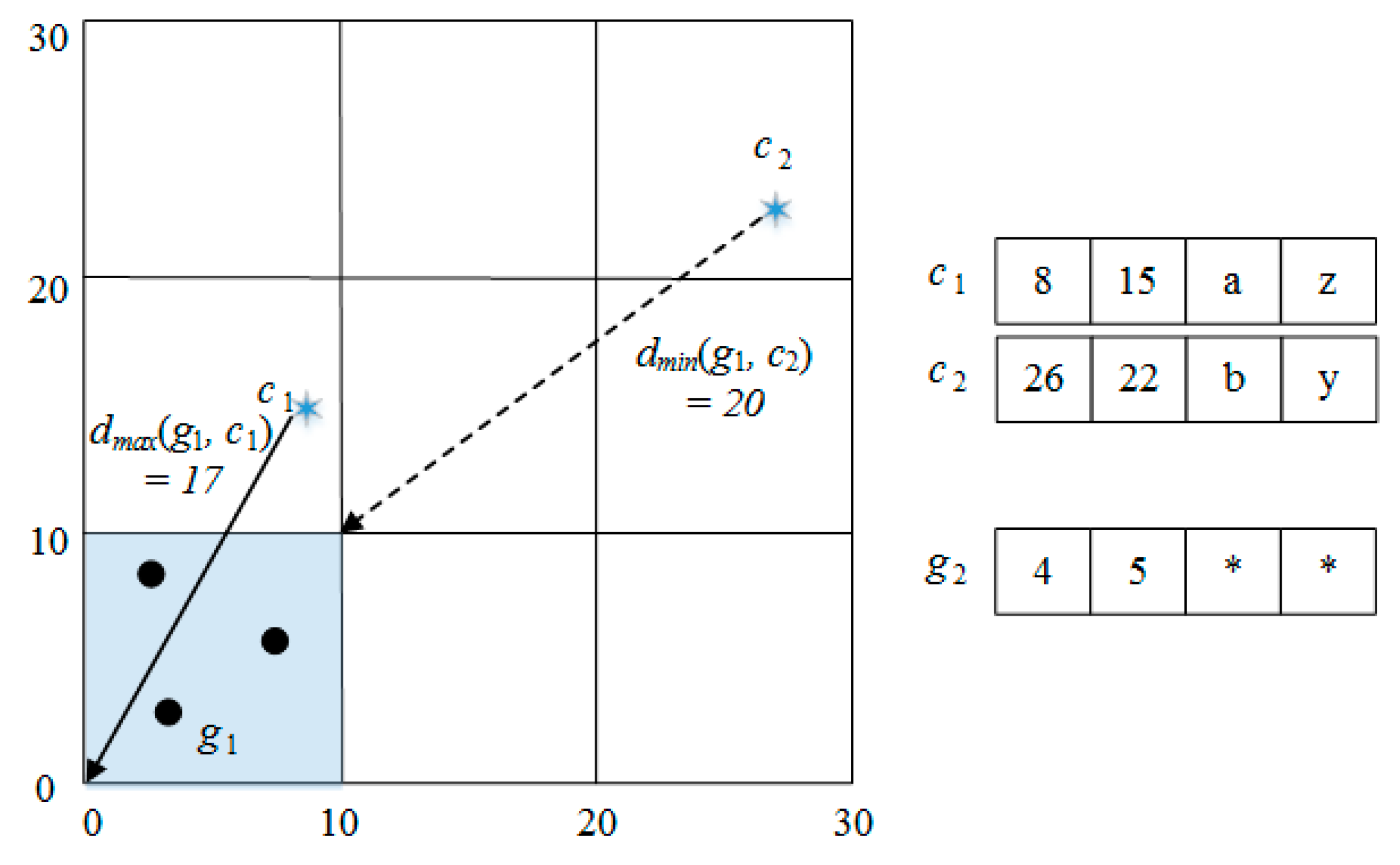
| dr(oi, cj) | a distance between an object and an cluster center for only numeric attributes |
| dc(oi, cj) | a distance between an object and an cluster center for only categorical attributes |
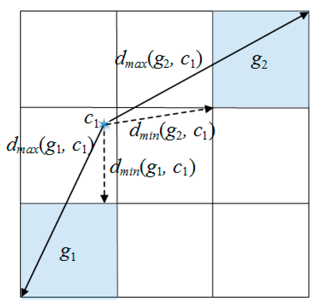
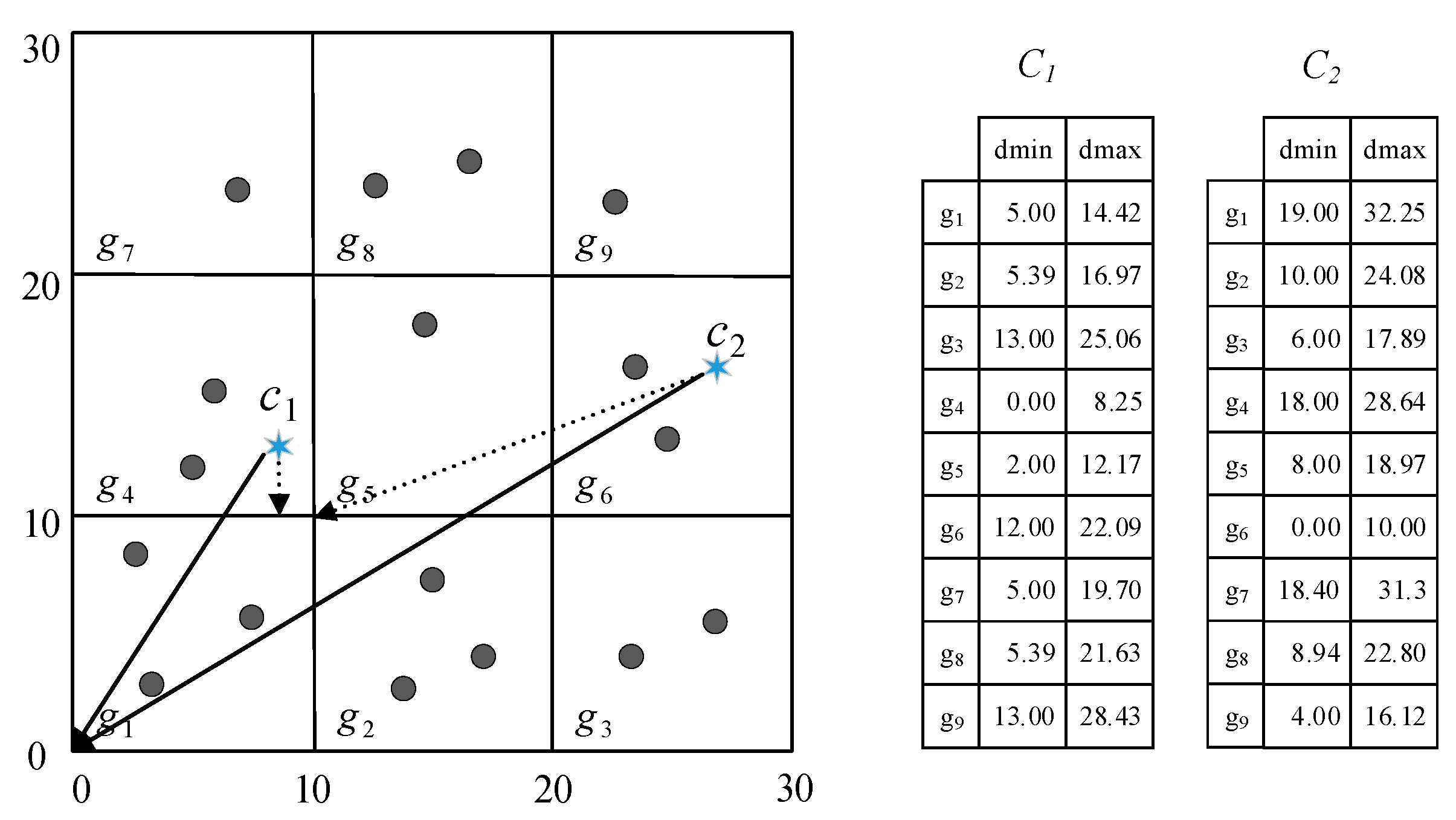
| dmin(gi, cj) | the minimum distance between a cell and a cluster center for only numeric attributes |
| dmax(gi, cj) | the maximum distance between a cell and a cluster center for only numeric attributes |
| Parameter | Description | Baseline Value |
|---|---|---|
| n | no. of objects | 1000 K |
| k | no. of clusters | 10 |
| mr | no. of numeric attributes | 2 |
| mc | no. of categorical attributes | 5 |
| s | no. of division in each dimensions | 10 |
© 2018 by the authors. Licensee MDPI, Basel, Switzerland. This article is an open access article distributed under the terms and conditions of the Creative Commons Attribution (CC BY) license (http://creativecommons.org/licenses/by/4.0/).
Share and Cite
Jang, H.-J.; Kim, B.; Kim, J.; Jung, S.-Y. An Efficient Grid-Based K-Prototypes Algorithm for Sustainable Decision-Making on Spatial Objects. Sustainability 2018, 10, 2614. https://doi.org/10.3390/su10082614
Jang H-J, Kim B, Kim J, Jung S-Y. An Efficient Grid-Based K-Prototypes Algorithm for Sustainable Decision-Making on Spatial Objects. Sustainability. 2018; 10(8):2614. https://doi.org/10.3390/su10082614
Chicago/Turabian StyleJang, Hong-Jun, Byoungwook Kim, Jongwan Kim, and Soon-Young Jung. 2018. "An Efficient Grid-Based K-Prototypes Algorithm for Sustainable Decision-Making on Spatial Objects" Sustainability 10, no. 8: 2614. https://doi.org/10.3390/su10082614
APA StyleJang, H.-J., Kim, B., Kim, J., & Jung, S.-Y. (2018). An Efficient Grid-Based K-Prototypes Algorithm for Sustainable Decision-Making on Spatial Objects. Sustainability, 10(8), 2614. https://doi.org/10.3390/su10082614