Morphological Precision Assessment of Reconstructed Surface Models for a Coral Atoll Lagoon

1
State Key Laboratory of Resources and Environmental Information System, Institute of Geographic Sciences and Natural Resources Research, Chinese Academy of Sciences, Beijing 100101, China
2
College of Resources and Environment, University of Chinese Academy of Sciences, Beijing 100049, China
3
School of Geography, Beijing Normal University, Beijing 100875, China
4
Department of Geographic Information Science, Nanjing University, Nanjing 210023, China
*
Author to whom correspondence should be addressed.
Sustainability 2018, 10(8), 2749; https://doi.org/10.3390/su10082749
Submission received: 15 June 2018
/
Revised: 21 July 2018
/
Accepted: 31 July 2018
/
Published: 3 August 2018
(This article belongs to the Special Issue Monitoring and Modelling Techniques for Sea Environment and Sustainable Development)
Abstract
:In addition to remote-sensing monitoring, reconstructing morphologic surface models through interpolation is an effective means to reflect the geomorphological evolution, especially for the lagoons of coral atolls, which are underwater. However, which interpolation method is optimal for lagoon geomorphological reconstruction and how to assess the morphological precision have been unclear. To address the aforementioned problems, this study proposed a morphological precision index system including the root mean square error (RMSE) of the elevation, the change rate of the local slope shape (CRLSS), and the change rate of the local slope aspect (CRLSA), and introduced the spatial appraisal and valuation approach of environment and ecosystems (SAVEE). In detail, ordinary kriging (OK), inverse distance weighting (IDW), radial basis function (RBF), and local polynomial interpolation (LPI) were used to reconstruct the lagoon surface models of a typical coral atoll in South China Sea and the morphological precision of them were assessed, respectively. The results are as follows: (i) OK, IDW, and RBF exhibit the best performance in terms of RMSE (0.3584 m), CRLSS (51.43%), and CRLSA (43.29%), respectively, while with insufficiently robust when considering all three aspects; (ii) IDW, LPI, and RBF are suitable for lagoon slopes, lagoon bottoms, and patch reefs, respectively; (iii) The geomorphic decomposition scale is an important factor that affects the precision of geomorphologic reconstructions; and, (iv) This system and evaluation approach can more comprehensively consider the differences in multiple precision indices.
1. Introduction
Coral reefs are some of the most productive and species-rich ecosystems on Earth. Currently, 275 million people living near coral reefs, which provide fisheries, oil and gas resources, and shoreline protection for communities [1]. Coral reefs also have very high tourist value [2], and many countries and regions benefit from the coral-reef tourism [1,3]. Many coral reefs also have important strategic value, and their key locations play unique roles in the division of territorial waters and exclusive economic zones in oceans [4]. However, coral reefs are suffering from a range of climatic and environmental changes, such as global warming, sea-level rise, ocean acidification, and typhoons [5,6,7,8], which can destroy coral reefs through extreme external stress [9,10,11]. In addition, coral reefs have suffered under the effects of human activities, including overfishing, destructive fishing, pollution, and habitat change due to coastal development, which have caused their degeneration [12,13,14]. The changes have affected the growth, transportation, degradation, and deposition of coral reefs, which have had important effects on their macro- and micro-morphological changes, causing the coral reefs to have highly dynamic geomorphology [15,16,17]. Therefore, the geomorphic evolution study of coral reefs is significant for their exploitation, protection, and management.
The evolution of geomorphology can be simulated by comparing the geomorphology of different periods. The basis of the simulating process is to reconstruct a highly precise surface model of the geomorphology at any time scale [18]. The data sources of morphological reconstructions are discrete and temporally and spatially limited, so appropriate reconstruction approaches are required in order to establish the continuous morphological surface model [18]. Since the 1970s, many scholars have proposed a series of interpolation methods for surface-model reconstruction, including polynomial interpolation, radial basis function interpolation, kriging interpolation, weighted average interpolation, triangle subdivision interpolation, and mathematical morphology interpolation, which have been widely used in many fields [19,20,21,22,23,24,25,26,27]. To evaluate the performance of reconstruction approaches for morphological surface models, many scholars have analyzed their respective advantages and disadvantages and their adaptability to different geomorphic types [28,29,30,31,32,33]. Because coral atoll reefs have spatial differentiation characteristics (i.e., “macroscopic ring-like continuous, microcosmic heterogeneous fragmentation”) [34], the previous empirical conclusions may not be applicable to a particular coral reef’s geomorphology, especially the lagoon geomorphic unit, which has various internal morphologies. Therefore, which reconstruction approaches is suitable for geomorphological reconstruction of coral atoll reefs has been unclear.
Moreover, the theory and technique of the morphological precision assessment still have some shortcomings. In many studies, the morphological precision assessment is limited to the precision of the elevation, and the root mean square error (RMSE) and mean error (ME) are always used as the main indices to measure the morphological precision [19,28,30,35,36,37,38]. However, Desmet and Govers defined the morphological precision as a compromise between numerical precision and shape reliability [39]. Wang et al. argued that morphological precision indices mainly include the closeness of the elevation surface, the similarity of local morphologies, and the compliance of local features [36]; these authors evaluated the morphological precision by using indices that contain the RMSE of the elevation and the correctness of the concave and convex characteristics of the local slope area. However, no accurate conceptual definition or mature quantitative analysis method currently exists for morphological precision.
The main objectives of this study are as follows: (1) establish a morphological precision assessment approach for reconstructed geomorphological surfaces and (2) evaluate the performance of the morphological reconstruction methods to select the optimal methods for coral atoll lagoon geomorphology. In this study, the change rate of the local slope aspect (CRLSA) is proposed to build an index system that combines the RMSE of the elevation and the change rate of the local slope shape (CRLSS), which is used to assess the morphological precision. The spatial appraisal and valuation of environment and ecosystems (SAVEE) is introduced to evaluate the performance of the reconstruction approaches. Four interpolation methods (inverse distance weighting, local polynomial interpolation, radial basis function interpolation, and ordinary Kriging interpolation), the selected conventional reconstruction approaches, are applied on a typical coral atoll in the Nansha Islands to reconstruct the lagoon geomorphic surface models. Specifically, robustness and geomorphic type adaptability of interpolation methods, effects of the geomorphic decomposition scale and potential and insufficiencies of the morphological precision index system are discussed to indicate the future work in this research.
2. Materials and Methods
2.1. Study Site and Datasets
The Nansha Islands (also known as the Spratly Islands in English) are located in the southern portion of the South China Sea (Figure 1a) and are dotted with islands, reefs, sands, and beaches, which cover an area of 880,000 km2. The coral reefs of the Nansha Islands can be classified as atolls, table reefs, patch reefs, etc., which are mainly atolls that are dominated by large atolls. Most of the Nansha Islands have a marine tropical rain-forest climate, with prevailing northeast and southwest monsoons. During the southwest monsoon season, the coral reefs are often affected by typhoons from the western Pacific, with dramatic morphological changes. In addition, the Nansha Islands have abundant fishery resources and oil and gas resources, and the islands’ coral reef ecosystems have been greatly affected as their exploitation increased in recent years.
We selected a typical atoll on the north of the Nansha Islands as the study site (Figure 1b), which is only exposed at low tide and whose forms are difficult to comprehensively obtain with remote-sensing images. Figure 1c shows the geomorphology of the lagoon at the study site. Its geomorphic units at the first-order scale (e.g., lagoon) were divided into geomorphic units at the second-order scale (e.g., lagoon slope, lagoon bottom, and patch reef), and the geomorphic units at the second-order scale (e.g., patch reef) were further decomposed into geomorphic units at the third-order scale (e.g., shallow patch reef and deep patch reef) based on the water depth (e.g., the top depths of the shallow patch reefs were less than 2 m) and shape (e.g., the top of the shallow patch reefs were relatively flat, and the deep patch reefs were always cone-shaped). The geomorphic subunits at all of the decomposition scales had various morphological characteristics.
We collected the bathymetry data from the study site in March 2012 to construct the surface models of the lagoon’s geomorphology. During the data collection, we conducted tidal corrections to ensure that the measurement results reflected the actual geomorphology of the lagoon as much as possible. During the data preprocessing, we detected and eliminated the gross errors in the data to ensure that the results were not affected. In addition, for the large amount of data, we used a 5-m grid for data thinning to facilitate the operation, after which we obtained the experimental dataset.
2.2. Interpolation Methods for the Morphology Surface Model Reconstruction
In this study, some commonly used deterministic and geostatistical interpolation methods were selected to construct the lagoon surface models, including inverse distance weighting (IDW), local polynomial interpolation (LPI), radial basis function interpolation (RBF), and ordinary kriging interpolation (OK). All of the above methods are based on the locations and values of the sampling points to estimate the values of unmeasured locations through mathematical functions or statistical models [31]. In addition, most GIS or data processing software integrates the above interpolation methods, which is convenient for us to study geomorphology. The “Geostatistical Wizard” tool in the “Geostatistical Analyst” tool set of ArcGIS 10.2 contains the above four interpolation methods, so we chose it as the experimental tool.
After selecting the interpolation methods, some parameter options that were related to the methods were identified, including the neighborhood type, search sectors, search neighbors, kernel function, and function variables. The interpolation parameters were the relative optimization parameters that were chosen by cross validation after several experiments. The parameter settings for each interpolation method are shown in Table 1.
2.3. Morphological Precision Assessment of the Surface Models
2.3.1. Assessment Approach of the Morphological Precision
An approach was designed to assess the precision of the morphology surface models, and the technical process of this assessment is shown in Figure 2. The following five procedures were adopted to analyze the morphological precision:
- (1)
- The original dataset was homogeneously diluted into a model training dataset (approximately 70%), which was used to reconstruct the surface models, and a model testing dataset (approximately 30%), which was used to validate the precision of the surface models and to extract the morphological errors.
- (2)
- A TIN surface model was reconstructed from the original dataset and converted into a grid surface model with a resolution of 1 m by using “TIN to Raster” tool in ArcGIS 10.2, to represent the true synthetic morphology.
- (3)
- Several grid surface models were reconstructed from the training dataset by IDW, LPI, RBF, and OK interpolation with a resolution of 1 m, to represent the estimated simulation morphology.
- (4)
- The morphological errors were calculated between the simulation morphology and synthetic morphology. The statistical morphological error was extracted from the testing dataset to conduct the precision assessment and error analysis.
- (5)
- The statistical morphological errors of the geomorphic subunits at different decomposition scales were extracted from the boundary and testing datasets to evaluate the precision of the surface models and the performance of the interpolation methods.
2.3.2. Morphological Precision Index System
In addition to the closeness of the elevation and changes in the concave and convex characteristics of the local slope surface, the morphological precision should be described to determine any aspect changes in the local slope surface. Therefore, this study inherited a change ratio for the concave and convex characteristics of the local slope surface, proposed a change ratio for the aspect characteristics of the local slope surface as the other morphological quantitative index, and reconstructed the morphological precision quantitative index system.
(1) Root mean square error (RMSE) of the elevation
The closeness of the elevation surface refers to the closeness between the simulated morphology surface and the synthetic morphology surface; this factor meets the basic requirements of random error by not introducing system error, so the root mean square error can be used in the quantitative description. The equation of RMSE can be expressed, as follows:
where Z is the observed elevation of the checkpoint in the synthetic surface model and Z* is the estimated elevation of the checkpoint in the simulation surface model.
(2) Change ratio of the local slope shape (CRLSS)
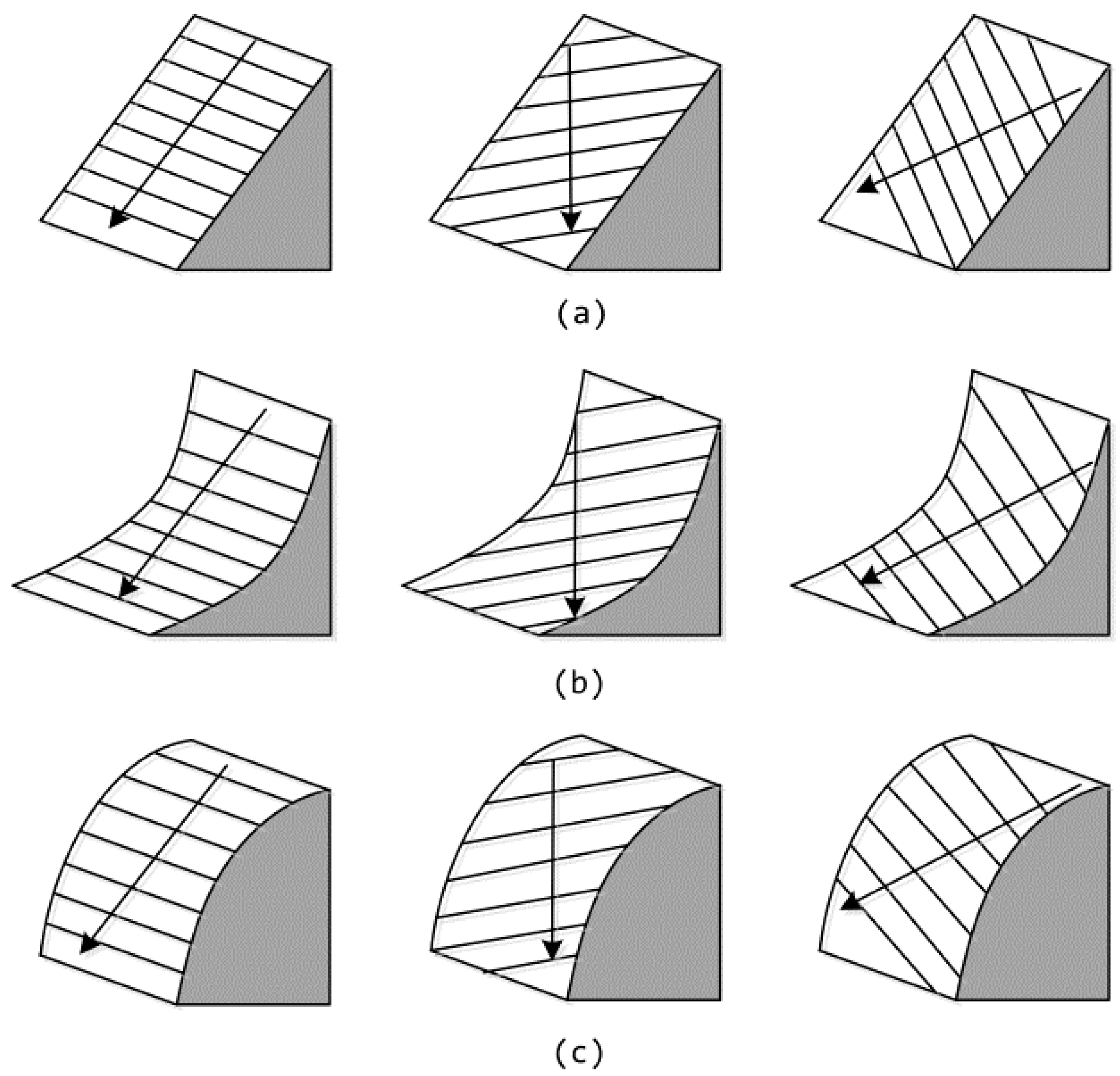
In terms of the morphology of the local slope shape, Tang [40] argues that any complex morphology surface can be decomposed into a flat slope (Figure 3a), concave slope (Figure 3b), and convex slope (Figure 3c). To some extent, this approach is equivalent to the reconstruction of high-precision geomorphology if every local slope shape can be accurately expressed when describing the geomorphology. Therefore, the precision of different surface models can be objectively analyzed by using the change ratio of the local slope shape as the precision index. The equation of CRLSS can be expressed, as follows:
where N is the number of checkpoints and Nc-ss is the number of changes in the local slope shape of all of the checked points.
The processing of slope shape statistics was, as follows [36].
- (i)
- Based on the synthetic surface model and the simulated surface models, which were recorded as “S”, the average value of the surface models was calculated by using the focal statistics tool in ArcGIS 10.2 with a 3 × 3 neighborhood analysis window, which was recorded as “Sm”.
- (ii)
- The raster calculator tool in ArcGIS 10.2 was used to subtract “S” from “Sm”, and the calculated results were recorded as “Sm-S”.
- (iii)
- “Sm-S” was reclassified into three local slope-shape types by using the raster calculator tool in ArcGIS10.2 based on the principle that the pixel value was greater than 0 for a concave slope, less than 0 for a convex slope, and equal to 0 for a flat slope; the result was recorded as “Ssm”.
- (iv)
- The local slope shapes of the morphology’s synthetic surface model and simulated surface models were extracted by using the testing dataset. In addition, the changed number or the proportion of the local slope shape of the simulated surface models relative to the synthetic surface model was counted to evaluate the precision (CRLSS) of the different simulated surface models.
(3) Change ratio of the local slope aspect (CRLSA)
The local slope aspect is also an important feature of the local geomorphology, such as local slopes with the same slope shape, which may have different slope aspects (Figure 4). In some cases, the morphological changes may not be reflected in the local slope shape but in the local slope aspect. Therefore, the CRLSA can also objectively reflect the precision of the morphology’s surface model. The equation of CRLSA can be expressed, as follows:
where N is the number of checkpoints and Nc-sa is the number of changes in the local slope shape of all of the checked points.
The processing of slope aspect statistics was, as follows.
- (i)
- Based on the synthetic surface model and the simulated surface models, the slope aspect of the surface models was calculated by using the aspect tool in ArcGIS 10.2, which were recorded as “Sa”. The slope aspect in ArcGIS software is measured in a clockwise direction, ranging from 0 (positive north) to 360 (still positive north), that is, a complete circle.
- (ii)
- “Sa” was reclassified into eight directions by using the raster calculator tool in ArcGIS10.2 based on the principle that the pixel value was greater than or equal to 0 and less than 22.5 for North, greater than or equal to 22.5 and less than 67.5 for Northeast, greater than or equal to 67.5 and less than 112.5 for East, greater than or equal to 112.5 and less than 157.5 for Southeast, greater than or equal to 157.5 and less than 202.5 for South, greater than or equal to 202.5 and less than 247.5 for Southeast, greater than or equal to 247.5 and less than 292.5 for West, greater than or equal to 292.5 and less than 337.5 for Northwest, greater than or equal to 337.5 and less than 360 for North; the result was recorded as “Sar”.
- (iii)
- The local slope aspects of the synthetic surface model and the simulated surface models were extracted by the testing dataset. In addition, the changed numbers or proportions of the local slope aspect between them were counted to evaluate the precision (CRLSA) of the different simulated surface models.
2.4. Performance Evaluation of the Interpolation Methods
To evaluate the performance of different interpolation methods, we should select a comprehensive evaluation approach that considers the various influencing factors to determine the optimal interpolation method for geomorphic types at different decomposition scales. Spatial Appraisal and Valuation of the Environment and Ecosystems (SAVEE) is a comprehensive evaluation system that can be applied to the values of multiple perspectives based on the concept of uncertainty reasoning; this approach was developed by the Ecological Science and Management department’s renewable resources application technology laboratory at Texas A&M University (STARR Lab). SAVEE has already obtained good evaluation results in forest management, landscape ecology, wildlife management, resource planning, reef spatial value evaluation, resource spatial value evaluation [41], and it has been continuously applied to new fields [42,43]. Therefore, SAVEE was introduced to evaluate the performance of different interpolation methods based on RMSE, CRLSS, and CRLSA.
The basic idea of SAVEE is to select appropriate factors and conduct standardized processing, so that each factor has a standardized value, which both reflects the relationship of the weight and embodies the value attribute of the factor itself. The factors can be compared to each other, and the influence of all the factors can be summed through the SAVEE operation formula, so that complex decision-making and evaluation problems can be expressed through numbers. The SAVEE method mainly includes the following steps:
(1) Data preparation
First, an optional subset can be set up based on the required data. In this study, a factor subset {RMSE, CRLSS, and CRLSA} was created based on the morphological precision index system.
(2) Data standardization
The standardization process converts all data to a value between (−1, 1). A value between (−1, 0) is a negative factor, which is harmful to the evaluation result. The factors that have a beneficial influence on the evaluation result are positive factors and they are represented by values between (0, 1). These factors are all positive influencing factors according to the properties of the precision indices, and the comprehensive evaluation value “V” decreases with an increase in the influencing factors “x”. The equation of data standardization can be expressed, as follows:
where V is the standardized value, x is the independent variable, and A is the boundary value of x.
(3) Superposition calculation (IAB)
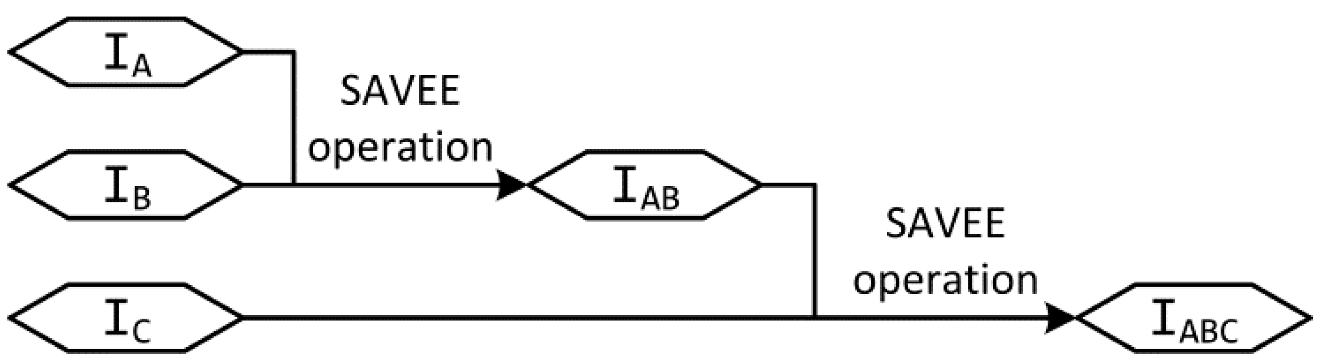
The SAVEE superposition equation is based on the EMYCIN formula, which is used to solve the equation of the superposition value of the influencing factors. EMYCIN is an “expert system” for building and developing expert systems. The concept that is defined by the EMYCIN formula itself is credibility. In this method, the superposition of the credibility is transformed into a superposition value of the influencing factors. Because the influencing factors are all positive, their values are all greater than 0. The superposition process of SAVEE is the repeated operation of the double factors until all of the factors are involved in the operation and the final result is the required superposition value. The calculation flow diagram is shown in Figure 5. The equation of superposition calculation can be expressed, as follows:
where the values of IA and IB are (−1, +1), IA is the standardized value of factor A, IB is the standardized value of factor B, and IAB is the superposition value of the factors A and B.
3. Results
Four lagoon morphology simulation surface models with a resolution of 1 m were reconstructed through IDW, LPI, RBF, and OK using the training dataset. A TIN surface model from the original data was converted to a synthetic grid surface model with a resolution of 1 m. Then, the elevation field models (Figure 6), local slope shape field models (Figure 7), and local slope aspect field models (Figure 8) of the lagoon were calculated for visual comparison, and several typical lagoon geomorphic subunits were selected as comparison objects for further local visual comparison.
3.1. Morphological Precision Comparison of the Lagoon Surface Models
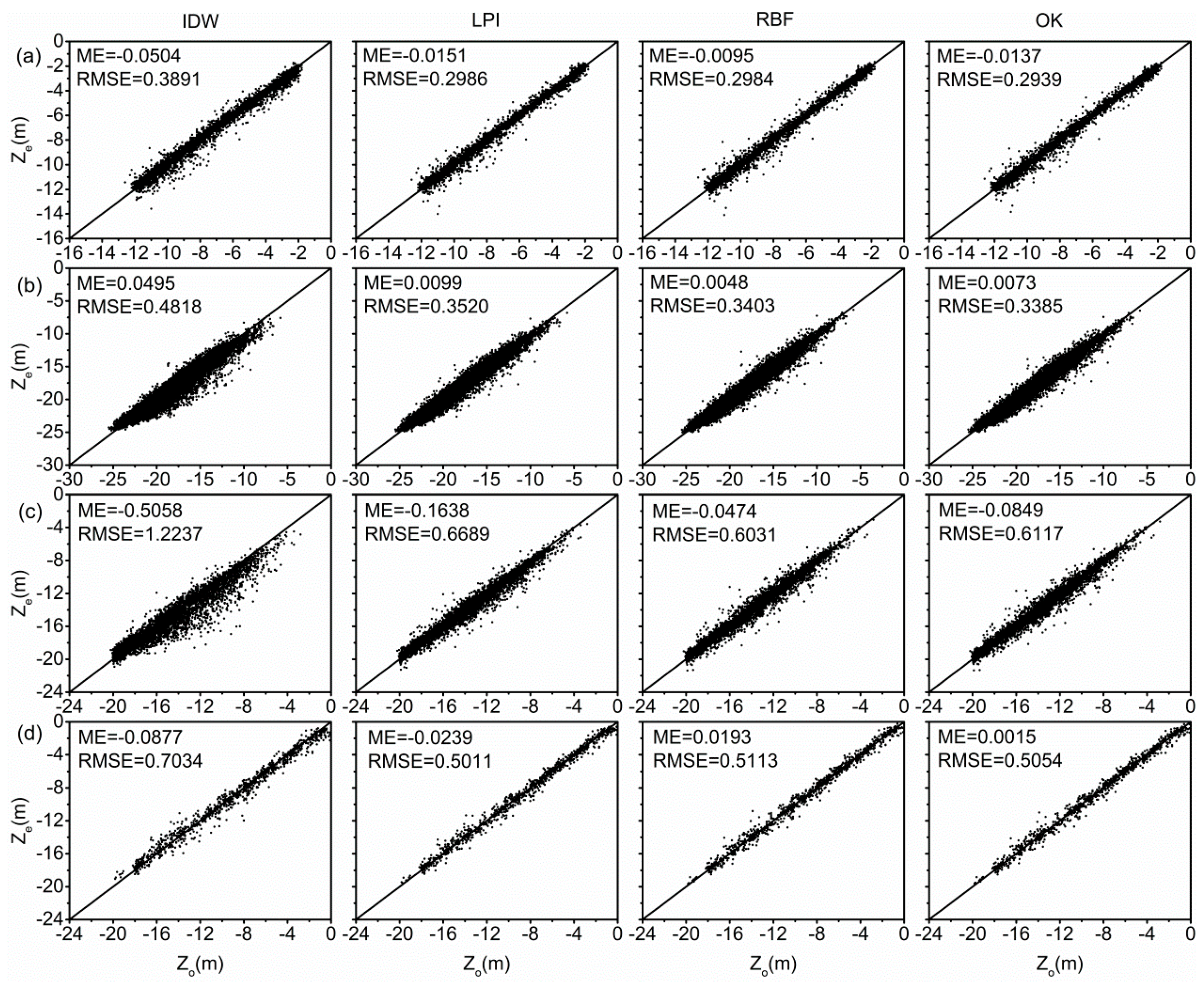
The elevation precision (RMSE) values of the surface models among OK, RBF, and LPI were relatively close; the surface model that was reconstructed by OK had the highest elevation precision, followed by RBF and LPI; IDW had the lowest elevation precision (Figure 9).
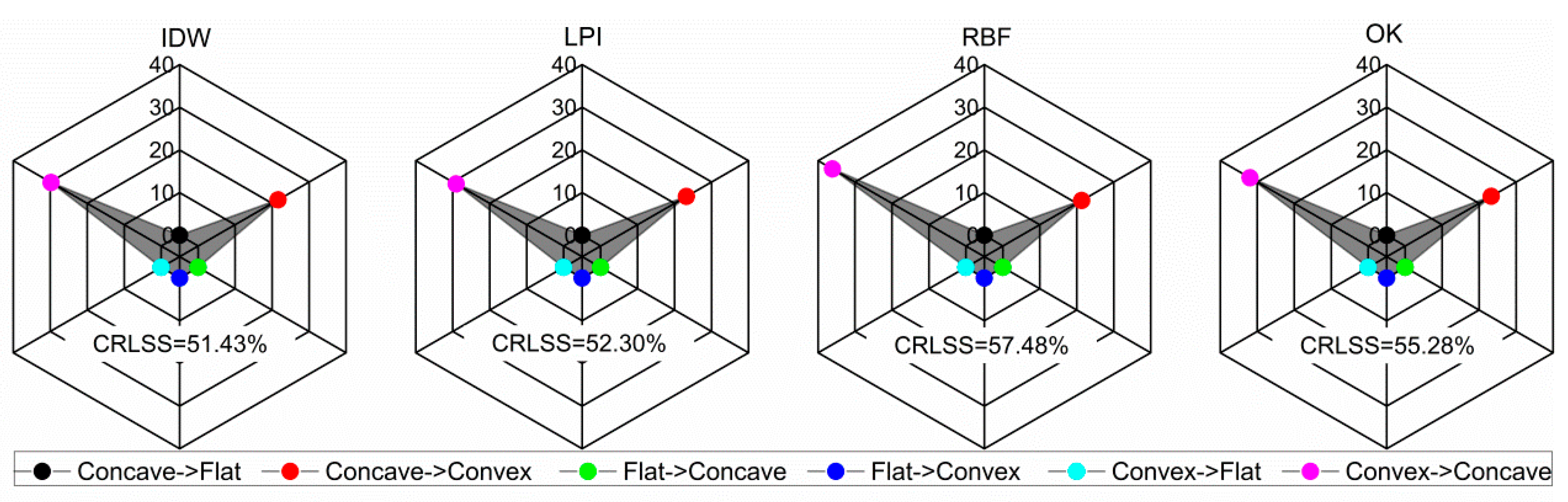
However, the statistical results of the local slope shape change (CRLSS) showed that the surface model that was reconstructed by IDW had the highest local slope shape precision, followed by LPI, OK, and RBF. According to the rule of local slope shape changes (Figure 10), the vast majority of slope shape changes existed between concave and convex slopes (called a “skip rank change”), and only a few changes existed between flat and concave slopes or between flat and convex slopes. The skip rank change rate of IDW was the lowest (51.41%), followed by LPI (52.28%) and OK (55.25%), while that of RBF was the highest (57.46%).
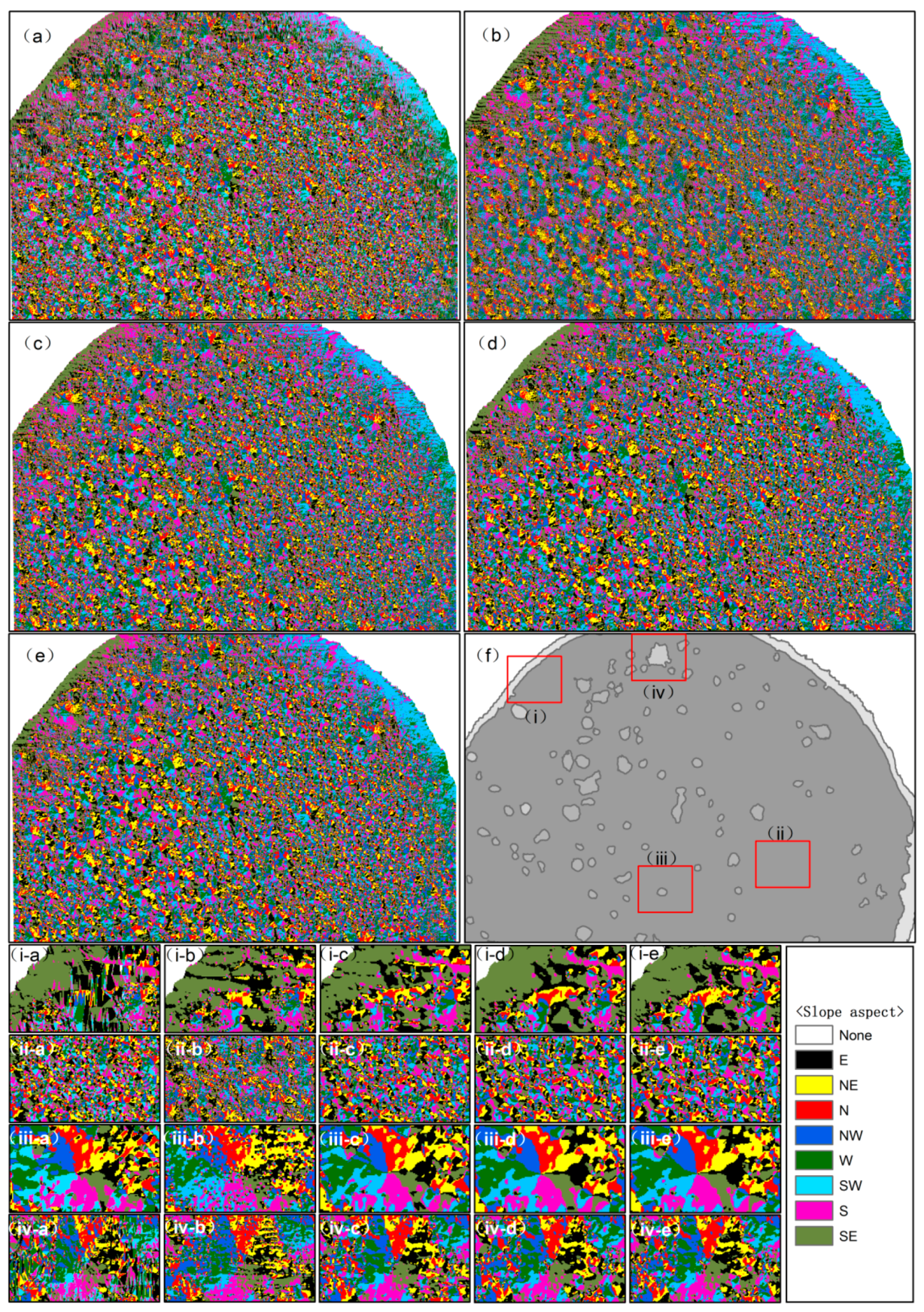
In addition, the surface model that was reconstructed by RBF had the highest local slope aspect precision (CRLSA), followed by OK, LPI, and IDW. According to the rule of local slope aspect changes (Figure 11), most of the changes occurred between the original slope aspect and its adjacent slope aspects, with very few changes between the original slope aspect and its opposite slope aspects (a “reverse change”). The reverse change rate of the RBF interpolation method was the lowest (4.27%), followed by OK (4.30%) and LPI (5.34%), while that of the IDW interpolation method was the highest (5.78%).
The quality of the surface models that were reconstructed by the interpolation methods was ordered by the morphological precision indices (Table 2). The four interpolation methods only had excellent performance for one morphological precision index, while with large differences occurring for the other three precision indices. For example, OK had the best performance in terms of RMSE but poor performance in terms of CRLSS. IDW had the best performance in terms of CRLSS but poor performance in terms of RMSE and CRLSA. RBF had the best performance in terms of CRLSA but the worst performance in terms of CRLSS. When considering the geomorphic characteristics, including the elevation, local slope shape, and local slope aspect, the performances of the four interpolation methods were not sufficiently robust.
3.2. Morphological Precision Comparison of the Lagoon Geomorphic Subunit Surface Models
The lagoon was divided into a lagoon slope, lagoon bottom, deep patch reef, and shallow patch reef, according to the second-order scale and third-order scale. The morphological errors of the surface models of the different geomorphic subunits were extracted, and the three morphological precision indices of RMSE, CRLSS, and CRLSA were analyzed.
According to the RMSE statistical results that are based on the surface models of different geomorphic subunits (Figure 12), the quality order of the lagoon slope surface models that were reconstructed by the interpolation methods was OK > RBF > LPI > IDW, which was consistent with the order of lagoon bottom. However, the quality order of the deep patch reef surface models was RBF > OK > LPI > IDW, and the quality order of the shallow patch reef surface models was LPI > OK > RBF > IDW.
From the CRLSS statistical results of the surface models of different geomorphic subunits (Figure 13), the quality order of the lagoon slope surface models was IDW > LPI > OK > RBF, which was consistent with the order of lagoon bottom. The quality order of the deep patch reef surface models was LPI > IDW > OK > RBF, and the quality order of the shallow patch reef surface models was IDW > OK > RBF > LPI.
According to the CRLSA statistical results of the surface models of different geomorphic subunits (Figure 14), the quality order of the lagoon slope surface models was RBF > OK > LPI > IDW, which was consistent with the order of lagoon bottom. The quality order of the deep patch reef surface models was OK > RBF> LPI > IDW, and the quality order of the shallow patch reef surface models was LPI > RBF > OK > IDW.
We obtained the mean morphological precision values of the surface models of different geomorphic subunits (Table 3). In terms of the mean RMSE value, the quality order was lagoon slope > lagoon bottom > shallow patch reef > deep patch reef. In terms of the mean CRLSS value, the quality order was lagoon bottom > lagoon slope > shallow patch reef > deep patch reef. In terms of the mean CRLSA value, the quality order was deep patch reef > shallow patch reef > lagoon slope > lagoon bottom. The morphological precision indices exhibited different anti-deformation abilities among different geomorphic subunits.
The above results showed that the unique morphological characteristics of the geomorphic subunits influenced the performance of the interpolation methods and determined the anti-deformation ability of the three morphological precision indices.
3.3. Adaptive Analysis of the Interpolation Methods for Lagoon Geomorphic Subunits
The comprehensive performance of different interpolation methods for constructing geomorphic subunit surface models was evaluated by the SAVEE method in order to determine the optimal interpolation method for different geomorphic subunits. First, the morphological precision index values were standardized, and a superposition calculation was implemented to obtain the comprehensive evaluation value.
According to the evaluation results (Table 4), the comprehensive performance of IDW in the lagoon slope, LPI in the lagoon bottom, RBF in the deep patch reef, and LPI in the shallow patch reef was optimal, respectively.
In addition, the comprehensive evaluation values of optimal interpolation methods between patch reef and shallow patch reef and deep patch reef were compared. As shown in Table 5, the optimal interpolation method of the patch reef at the second-order geomorphic scale was RBF, while the deep patch reef and shallow patch reef at the third-order geomorphic scale were RBF and LPI, respectively. This shows that different decomposition scales have a large influence on the determination of the optimal interpolation method of geomorphic subunits, which will influence the morphological precision of the reconstructed surface model.
4. Discussion
4.1. Robustness and Geomorphic Type Adaptability of Interpolation Methods
The performance of the several interpolation methods that were used in this study were better in terms of individual indices, but not sufficiently robust of synthesizing other indices. Ordinary kriging (OK), as a type of Kriging, has very high fitting precision in elevation (RMSE of elevation) and it is always preferred modeling method in many practical applications [28,29,30,31,32,33,44,45,46]. However, the high numerical precision also exists the phenomenon of over-fitting [47,48,49]. With the application of OK to obtain a high elevation numerical precision, the local morphology of the surface model may change, such as a concave slope becomes a convex one, thus causing the change of slope aspect. RBF fits a minimum-curvature surface through the input points, and ensure the preservation of trend in the sample data along with rapid changes in gradient or slope [30], which enables it to maintain relatively good local slope aspect precision. In most cases, RBF is similar to geostatistical interpolation, and it also has the smoothing effect when obtaining better elevation numerical precision [28,29,30,31,45]. In previous studies, elevation numerical precision of IDW is lower than OK, RBF, or other interpolation methods [25,28,30,31,32,50]. The maximum and minimum values of the surface model constructed by IDW can only be found at the sampling point [39,43,51], which reduces the over-fitting of unknown points to a certain extent, so that it performs well in the shape precision of local slope.
The shape of the lagoon slope is inclined, mainly composed of fine coral sand with relatively flat and smooth surface [52]. IDW have been found to be good for interpolation of geo-morphologically smooth areas [30]. When compared with other methods, IDW has no significant difference in elevation numerical precision, and it has a higher shape precision of local slope. Therefore, IDW is superior to other methods in the comprehensive evaluation of geomorphic adaptability of lagoon slope. Shallow patch reefs generally have flat tops and are similar to the bottom of lagoons in macroscopic morphology [34]. At the micro level, the surface of shallow patch reef is full of coral reefs, and the lagoon bottom is composed of coarse grained coral gravel and coral sand, all of which have certain characteristics of local relief [34,52]. From the results, the comprehensive evaluation values of LPI, RBF, and OK in the geomorphic adaptability of shallow patch reef and lagoon bottom are similar, but LPI is better than them. On the one hand, LPI method can reflect trend changes in all data points; on the other hand, it has the advantages of reflecting local features and making local smooth surface [53]. The deep patch reef is conical-shaped [52], and the change of local slope aspect is the main factor affecting the simulation precision. The comprehensive evaluation value of OK is close to RBF, but the characteristics of RBF make it more suitable for morphological simulation of deep patch reef. When this morphological index system is considered comprehensively, OK is not the optimal interpolation method for any lagoon geomorphic subunit. The main reason is that when OK extremely approaches the macroscopic morphology as much as possible, the over-fitting effect causes the distortion of local morphology.
In fact, it is very difficult to use a formula to accurately express the natural morphological surface, so it can only make the simulated surface as close as possible to the natural surface. Currently, there have been many studies on the adaptability of geomorphic types of interpolation methods [29,30,31,38,47]. Some scholars have also studied the problem of over-fitting correction of interpolation methods, and put forward some feasible improvement methods, such as cross validation [47,48,49]. However, it is well known that the optimal interpolation method for different geomorphic types is relative, which means that no interpolation method is absolutely suitable for a geomorphic type. In addition, the interpolation methods that were used in this study are common in other fields, and the optimal interpolation method of each lagoon geomorphic unit may be different if other interpolation methods are involved in model building. In order to construct a surface model with morphological fidelity, we need to further the study of surface model reconstruction methods.
4.2. Effect of the Geomorphic Decomposition Scale
When the geomorphology is decomposed at different scales, the final reconstruction surface model will be different and will further affect the reconstruction approaches. For example, as shown in Table 5, patch reef at the second-order geomorphic scale was further decomposed into shallow patch reef and deep patch reef, so there were differences in the morphological precision and optimal construction methods of the final surface model. Essentially, these differences in morphological precision and optimal construction method are caused by the difference of local morphology between the shallow patch reef and the deep patch reef.
In the previous studies, morphological features, the sampling point density and distribution, and different interpolation parameters all have a large influence on the performance of interpolation methods and morphological surface precision [28,31,37]. Among them, geomorphic type determines the difficulty of surface expression. However, the effect of this difference on morphological surface reconstruction is mostly discussed at the same geomorphic scale [29,30,31,38,50]. In this study, the differences in surface morphology between patch reef and lagoon slope and lagoon bottom were compared at the same scale as previous studies, while that between patch reef and shallow patch reef and deep patch reef were compared at different geomorphic scales. Comparison results show that we should pay attention to the influence of geomorphic decomposition scales on the surface morphological reconstruction in the actual production process.
In theory, geomorphic types can be infinitely decomposed as long as reasonable and effective decomposition bases or methods exist. However, further decomposing a geomorphic unit becomes difficult after it has been decomposed to a certain extent. Therefore, it is necessary to further establish the decomposing signs or indicators of the geomorphic types at different scales.
4.3. Potential and Shortcomings of the Morphological Precision Index System
Research on surface-model precision has been ongoing, but it has mostly focused on the numerical precision of the elevation in the surface model [19,28,30,35,36,37,38], and a few studies have considered shape reliability [31,36,54]. From the perspective of morphological characteristics, the numerical precision of elevation is only a measure of the elevation dispersion degree of points. This study proposed that any morphological characteristics can be expressed by “point, line and area” as the three main features. Therefore, when combined with the RMSE of the elevation (to measure the elevation dispersion degree of points) and local slope shape error (to measure the concave and convex properties of areas), the local slope aspect error (to measure the direction change of lines) was proposed to build a morphological precision index system. When compared to many previous studies, the morphological precision index system established in this study is a more comprehensive system. For another, the proposed morphological precision index system was combined with the SAVEE method, which provides an approach for the reconstruction methods optimization of surface model by considering the multi-index differences.
Furthermore, the precision index system has been applied well in the morphological precision assessment of the lagoon. We consider that this technique can be also applied to the morphological precision assessment of other research fields, such as the surface erosion, deposition change, and the precision assessment of terrain sampling data thinning.
However, many questions remain regarding the quality connotation and assessment method of the surface model, such as the morphological precision of the simulated geomorphology surface model and how this value be quantified. The morphological index system in this study does not represent a complete system. It is a comprehensive system, and other indices representing morphological changes should be considered. Therefore, both the theories and approaches of assessing geomorphological precision require further research.
5. Conclusions
Understanding the geomorphic evolution of coral reefs requires reconstructing their morphological surface models. However, it is unclear which method is optimal for lagoon geomorphological reconstruction, and the theory and technique are currently not yet sufficient to assess morphological precision. Therefore, this study designed a morphological precision index system and evaluation approach. The lagoon geomorphic unit of a typical atoll in the Nansha Islands was used as the experimental object. Surface models of the lagoon’s geomorphology were established by several conventional interpolation methods, and precision assessment and performance evaluations were conducted. The key findings in this study were as follows:
- (1)
- OK had the best performance in terms of RMSE but poor performance of CRLSS. IDW had the best performance in terms of CRLSS but poor performance of RMSE and CRLSA. RBF had the best performance in terms of CRLSA, but the worst performance of CRLSS. The performance of these interpolation methods was not sufficiently robust in the morphological reconstruction of lagoons. Because of their unique morphological characteristics, the surface models of the lagoon’s geomorphic subunits had various quality orders in the three of the morphological precision indices, indicating large differences in morphological precision among the lagoon’s geomorphic subunits. The morphological characteristics of the lagoon’s geomorphic subunits determined their anti-deformation ability in the three morphological precision indices when reconstructing morphological surface models.
- (2)
- The adaptive analysis results showed that IDW was the optimal method for lagoon slopes, LPI was the best method for lagoon bottoms and shallow patch reefs, and RBF was better than the other methods for deep patch reefs. Previous studies generally showed that kriging was superior to other interpolation methods in many fields, but kriging was not the optimal interpolation method for any of the lagoon’s geomorphic subunits when being measured by the morphological precision index system.
- (3)
- In addition to morphological features, the sampling point density and distribution, and different interpolation parameters, the geomorphic decomposition scale was an important factor affecting the reconstruction precision, which greatly affects the determination of the optimal interpolation method for geomorphic subunits and the morphological precision of the reconstructed surface models.
- (4)
- The proposed morphological precision index system can assess the morphological precision of reconstructed surface models more comprehensively from three aspects: the dispersion degree of the point, the direction accuracy of the line, and the shape accuracy of the area. This system can reflect the differences in reconstruction ability of interpolation methods in local morphologies. SAVEE can evaluate the performance of the reconstruction methods comprehensively by considering the differences in multiple precision indices. These methods extend the theory and method of morphological precision assessment and can be applied to other research fields. In future research, the morphological precision assessment theory and the new reconstruction approaches will be important directions for the theoretical research on geomorphological reconstruction.
Author Contributions
All the authors contributed to this manuscript. F.S. proposed the research, Q.W. designed the experiment and wrote the manuscript, Y.Z. and H.J. provided the language help, F.C. edited the manuscript.
Funding
This research was funded by the National Natural Science Foundation of China (Grant Number: 41421001) and the Strategic Priority Research Program of the Chinese Academy of Sciences (Grant Number: XDA13010403).
Acknowledgments
The authors gratefully acknowledge the financial supports by the National Natural Science Foundation of China (Grant Number: 41421001) and the Strategic Priority Research Program of the Chinese Academy of Sciences (Grant Number: XDA13010403).
Conflicts of Interest
The authors declare no conflict of interest.
References
- Jaleel, A. The status of the coral reefs and the management approaches: The case of the Maldives. Ocean Coast. Manag. 2013, 82, 104–118. [Google Scholar] [CrossRef]
- Moberg, F.; Folke, C. Ecological goods and services of coral reef ecosystems. Ecol. Econ. 1999, 29, 215–233. [Google Scholar] [CrossRef]
- Parzen, M.; Lipsitz, S.R. A meta-analysis of reef island response to environmental change on the Great Barrier Reef. Earth Surf. Process. Landf. 2015, 40, 1006–1016. [Google Scholar]
- Zhao, H.; Wang, L.; Yuan, J. Sustainable Development of the Coral Reefs in the South China Sea Islands. Trop. Geogr. 2016, 36, 55–65. (In Chinese) [Google Scholar]
- Coles, S.L.; Looker, E.; Burt, J.A. Twenty-year changes in coral near Muscat, Oman estimated from manta board tow observations. Mar. Environ. Res. 2015, 103, 66–73. [Google Scholar] [CrossRef] [PubMed]
- Hughes, T.P.; Huang, H.; Young, M.A.L. The Wicked Problem of China’s Disappearing Coral Reefs. Conserv. Biol. 2013, 27, 261–269. [Google Scholar] [CrossRef] [PubMed]
- Lapointe, B.E.; Thacker, K.; Hanson, C.; Getten, L. Sewage pollution in Negril, Jamaica: Effects on nutrition and ecology of coral reef macroalgae. Chin. J. Oceanol. Limnol. 2011, 29, 775–789. [Google Scholar] [CrossRef]
- Mcwilliams, J.P.; Côté, I.M.; Gill, J.A.; Sutherland, W.J.; Watkinson, A.R. Accelerating impacts of temperature-induced coral bleaching in the caribbean. Ecology 2005, 86, 2055–2060. [Google Scholar] [CrossRef]
- Kayanne, H.; Aoki, K.; Suzuki, T.; Hongo, C.; Yamano, H.; Ide, Y.; Iwatsuka, Y.; Takahashi, K.; Katayama, H.; Sekimoto, T.; et al. Eco-geomorphic processes that maintain a small coral reef island: Ballast Island in the Ryukyu Islands, Japan. Geomorphology 2016, 271, 84–93. [Google Scholar] [CrossRef]
- Perry, C.T.; Smithers, S.G.; Kench, P.S.; Pears, B. Impacts of Cyclone Yasi on nearshore, terrigenous sediment-dominated reefs of the central Great Barrier Reef, Australia. Geomorphology 2014, 222, 92–105. [Google Scholar] [CrossRef]
- Liu, G.; Strong, A.E.; Skirving, W. Remote sensing of sea surface temperatures during 2002 Barrier Reef coral bleaching. Eos Trans. Am. Geophys. Union 2003, 84, 137–141. [Google Scholar] [CrossRef]
- Palandro, D.A.; Andréfouët, S.; Hu, C.; Hallock, P.; Müller-Karger, F.E.; Dustan, P.; Callahan, M.K.; Kranenburg, C.; Beaver, C.R. Quantification of two decades of shallow-water coral reef habitat decline in the Florida Keys National Marine Sanctuary using Landsat data (1984–2002). Remote Sens. Environ. 2008, 112, 3388–3399. [Google Scholar] [CrossRef]
- Rogers, C.; Miller, J. Permanent ‘phase shifts’ or reversible declines in coral cover? Lack of recovery of two coral reefs in St. John, US Virgin Islands. Mar. Ecol. Prog. 2006, 306, 103–114. [Google Scholar] [CrossRef]
- Hoegh-Guldberg, O. Climate change, coral bleaching and the future of the world’s coral reefs. Mar. Freshw. Res. 1999, 50, 839–866. [Google Scholar] [CrossRef]
- Duvat, V.K.E.; Pillet, V. Shoreline changes in reef islands of the Central Pacific: Takapoto Atoll, Northern Tuamotu, French Polynesia. Geomorphology 2017, 282, 96–118. [Google Scholar] [CrossRef]
- Mann, T.; Westphal, H. Multi-decadal shoreline changes on Takú Atoll, Papua New Guinea: Observational evidence of early reef island recovery after the impact of storm waves. Geomorphology 2016, 257, 75–84. [Google Scholar] [CrossRef]
- Duce, S.; Vila-Concejo, A.; Hamylton, S.M.; Webster, J.M.; Bruce, E.; Beaman, R.J. A morphometric assessment and classification of coral reef spur and groove morphology. Geomorphology 2016, 265, 68–83. [Google Scholar] [CrossRef]
- Xu, S.Y.; Sun, Y.Y. Computer aided geomorphologic simulation. Acta Geogr. Sin. 2000, 55, 266–273. (In Chinese) [Google Scholar]
- Chen, C.; Liu, F.; Li, Y.; Yan, C.; Liu, G. A robust interpolation method for constructing digital elevation models from remote sensing data. Geomorphology 2016, 268, 275–287. [Google Scholar] [CrossRef]
- Hu, H.; Shu, H. An improved coarse-grained parallel algorithm for computational acceleration of ordinary Kriging interpolation. Comput. Geosci. 2015, 78, 44–52. [Google Scholar] [CrossRef]
- Chen, C.; Li, Y. A robust method of thin plate spline and its application to DEM construction. Comput. Geosci. 2012, 48, 9–16. [Google Scholar] [CrossRef]
- Erdoğan, S. Modelling the spatial distribution of DEM error with geographically weighted regression: An experimental study. Comput. Geosci. 2010, 36, 34–43. [Google Scholar] [CrossRef]
- Chen, C.; Yue, T. A method of DEM construction and related error analysis. Comput. Geosci. 2010, 36, 717–725. [Google Scholar] [CrossRef]
- Bater, C.W.; Coops, N.C. Evaluating error associated with lidar-derived DEM interpolation. Comput. Geosci. 2009, 35, 289–300. [Google Scholar] [CrossRef]
- Lu, G.Y.; Wong, D.W. An adaptive inverse-distance weighting spatial interpolation technique. Comput. Geosci. 2008, 34, 1044–1055. [Google Scholar] [CrossRef]
- Yu, Z.W. Surface interpolation from irregularly distributed points using surface splines, with Fortran program. Comput. Geosci. 2001, 27, 877–882. [Google Scholar] [CrossRef]
- Bartier, P.M.; Keller, C.P. Multivariate interpolation to incorporate thematic surface data using inverse distance weighting (IDW). Comput. Geosci. 1996, 22, 795–799. [Google Scholar] [CrossRef]
- Ding, Q.; Wang, Y.; Zhuang, D. Comparison of the common spatial interpolation methods used to analyze potentially toxic elements surrounding mining regions. J. Environ. Manag. 2018, 212, 23–31. [Google Scholar] [CrossRef] [PubMed]
- Geach, M.R.; Stokes, M.; Telfer, M.W.; Mather, A.E.; Fyfe, R.M.; Lewin, S. The application of geospatial interpolation methods in the reconstruction of Quaternary landform records. Geomorphology 2014, 216, 234–246. [Google Scholar] [CrossRef]
- Arun, P.V. A comparative analysis of different DEM interpolation methods. Egypt. J. Remote Sens. Space Sci. 2013, 16, 133–139. [Google Scholar]
- Chaplot, V.; Darboux, F.; Bourennane, H.; Leguédois, S.; Silvera, N.; Phachomphon, K. Accuracy of interpolation techniques for the derivation of digital elevation models in relation to landform types and data density. Geomorphology 2006, 77, 126–141. [Google Scholar] [CrossRef]
- Zimmerman, D.; Pavlik, C.; Ruggles, A.; Armstrong, M.P. An Experimental Comparison of Ordinary and Universal Kriging and Inverse Distance Weighting. Math. Geol. 1999, 31, 375–390. [Google Scholar] [CrossRef]
- Laslett, G.M.; Mcbratney, A.B. Further comparison of spatial methods for predicting soil pH. Soil Sci. Soc. Am. J. 1990, 54, 1553–1558. [Google Scholar] [CrossRef]
- Zhou, M.; Liu, Y.; Manchun, L.I.; Sun, C.; Wei, Z. Geomorphologic information extraction for multi-objective coral islands from remotely sensed imagery: A case study for Yongle Atoll, South China Sea. Geogr. Res. 2015, 34, 677–690. (In Chinese) [Google Scholar]
- Wise, S. Cross-validation as a means of investigating DEM interpolation error. Comput. Geosci. 2011, 37, 978–991. [Google Scholar] [CrossRef]
- Wang, C.; Liu, X.J.; Tang, G.A.; Tao, Y. Morphologic Fidelity of Grid Digital Elevation Model. Geomat. Inf. Sci. Wuhan Univ. 2009, 34, 146–149. (In Chinese) [Google Scholar]
- Heritage, G.L.; Milan, D.J.; Large, A.R.G.; Fuller, I.C. Influence of survey strategy and interpolation model on DEM quality. Geomorphology 2009, 112, 334–344. [Google Scholar] [CrossRef]
- Aguilar, F.J. Effects of Terrain Morphology, Sampling Density, and Interpolation Methods on Grid DEM Accuracy. Photogramm. Eng. Remote Sens. 2005, 71, 805–816. [Google Scholar] [CrossRef]
- Desmet, P.J.J.; Govers, G. Two-dimensional modelling of the within-field variation in rill and gully geometry and location related to topography. Catena 1997, 29, 283–306. [Google Scholar] [CrossRef]
- Tang, G. Progress of DEM and digital terrain analysis in China. Acta Geogr. Sin. 2014, 69, 1305–1325. (In Chinese) [Google Scholar]
- Loh, D.K.; Ytc, H.; Choo, Y.K.; Holtfrerich, D.R. Integration of a rule-based expert system with GIS through a relational database management system for forest resource management. Comput. Electron. Agric. 1994, 11, 215–228. [Google Scholar] [CrossRef]
- Chen, S.Y.; Cheng, Z.Y.; Loh, D.K. Islands valuation of spatial appraisal based on SAVEE method—With the Nansha Islands as an example. Mar. Environ. Sci. 2012, 31, 107–110. (In Chinese) [Google Scholar]
- Loh, D.K.; Stipdonk, S.E.P.V.; Holtfrerich, D.R.; Hsieh, Y.T.C. Spatially constrained reasoning for the determination of wildlife foraging areas. Comput. Electron. Agric. 1996, 15, 323–334. [Google Scholar] [CrossRef]
- Wilson, J.; Gallant, J. Digital Terrain Analysis in Terrain Analysis: Principles and Applications; Wiley: New York, NY, USA, 2000; Volume 479, pp. 1–27. [Google Scholar]
- Laslett, G. Kriging and Splines: An Empirical Comparison of their Predictive Performance in Some Applications. J. Am. Stat. Assoc. 1994, 89, 391–400. [Google Scholar] [CrossRef]
- Creutin, J.D.; Obled, C. Objective analyses and mapping techniques for rainfall fields: An objective comparison. Water Resour. Res. 1982, 18, 413–431. [Google Scholar] [CrossRef]
- Zhang, T.; Xu, X.; Xu, S. Method of establishing an underwater digital elevation terrain based on kriging interpolation. Measurement 2015, 63, 287–298. [Google Scholar] [CrossRef]
- Rezaee, H.; Asghari, O.; Yamamoto, J.K. On the reduction of the ordinary kriging smoothing effect. J. Min. Environ. 2011, 2, 25–40. [Google Scholar]
- Yamamoto, J.K. Correcting the Smoothing Effect of Ordinary Kriging Estimates. Math. Geol. 2005, 37, 69–94. [Google Scholar] [CrossRef]
- Erdoğan, S. A comparision of interpolation methods for producing digital elevation models at the field scale. Earth Surf. Process. Landf. 2009, 34, 366–376. [Google Scholar] [CrossRef]
- Watson, D.F. A refinement of inverse distance weighted interpolation. Geo-Processing 1985, 2, 315–327. [Google Scholar]
- Sun, Z.; Zhao, H. Features of dynamic geomorphology of coral reefs in nansha islands. Trop. Oceanol. 1996. (In Chinese) [Google Scholar]
- Yilmaz, H.M. The effect of interpolation methods in surface definition: An experimental study. Earth Surf. Process. Landf. 2007, 32, 1346–1361. [Google Scholar] [CrossRef]
- Desmet, P.J.J. Effects of Interpolation Errors on the Analysis of DEMs. Earth Surf. Process. Landf. 2015, 22, 563–580. [Google Scholar] [CrossRef]
Figure 1.
Study site: (a) Location of the Nansha Islands. (b) Satellite image of the study site. (c) Geomorphology of the lagoon at the study site.
Figure 1.
Study site: (a) Location of the Nansha Islands. (b) Satellite image of the study site. (c) Geomorphology of the lagoon at the study site.

Figure 2.
Technical process of the morphological precision assessment.

Figure 3.
Schematic diagram of local slope shapes: (a) flat slope, (b) concave slope, and (c) convex slope.
Figure 3.
Schematic diagram of local slope shapes: (a) flat slope, (b) concave slope, and (c) convex slope.

Figure 4.
Schematic diagram of local slopes with different aspects: (a) flat slope with different aspects, (b) concave slope with different aspects, and (c) convex slope with different aspects.
Figure 4.
Schematic diagram of local slopes with different aspects: (a) flat slope with different aspects, (b) concave slope with different aspects, and (c) convex slope with different aspects.

Figure 5.
Superposition process of the influencing factors in the spatial appraisal and valuation of environment and ecosystems (SAVEE) evaluation.
Figure 5.
Superposition process of the influencing factors in the spatial appraisal and valuation of environment and ecosystems (SAVEE) evaluation.

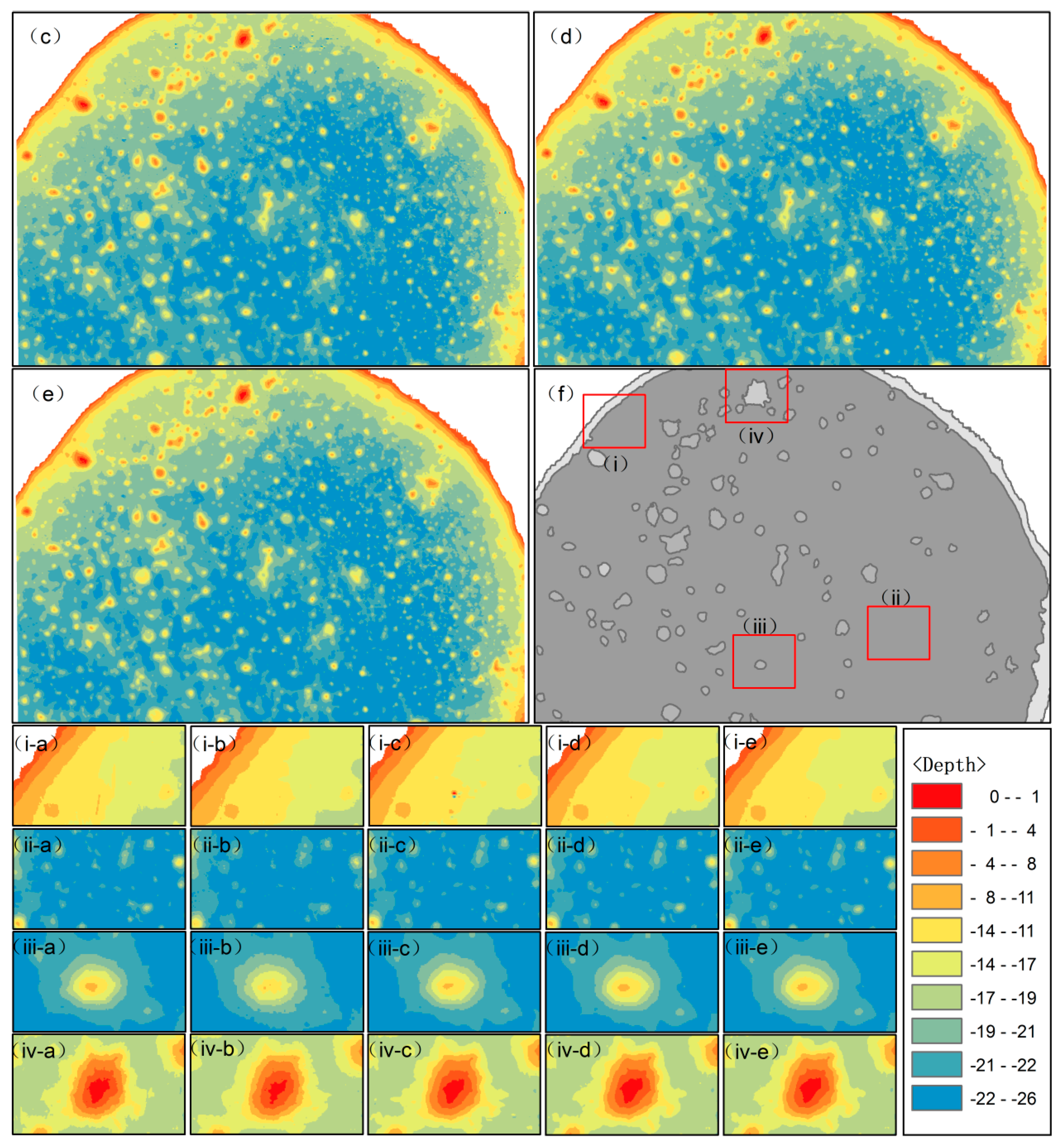
Figure 6.
Elevation field models of the lagoon. The first elevation field model was generated from the synthetic surface model from (a) TIN, and the others were generated from the simulated surface models that were reconstructed by (b) inverse distance weighting (IDW), (c) local polynomial interpolation (LPI), (d) radial basis function interpolation (RBF), and (e) ordinary kriging (OK). The Pattern areas were selected from (f) the lagoon’s geomorphic subunits for further comparison: (i) lagoon slope, (ii) lagoon bottom, (iii) deep patch reef, and (iv) shallow patch reef. These patterns (i-a–iv-e) reflect the differences in the simulated and synthetic surfaces in the elevation field model.


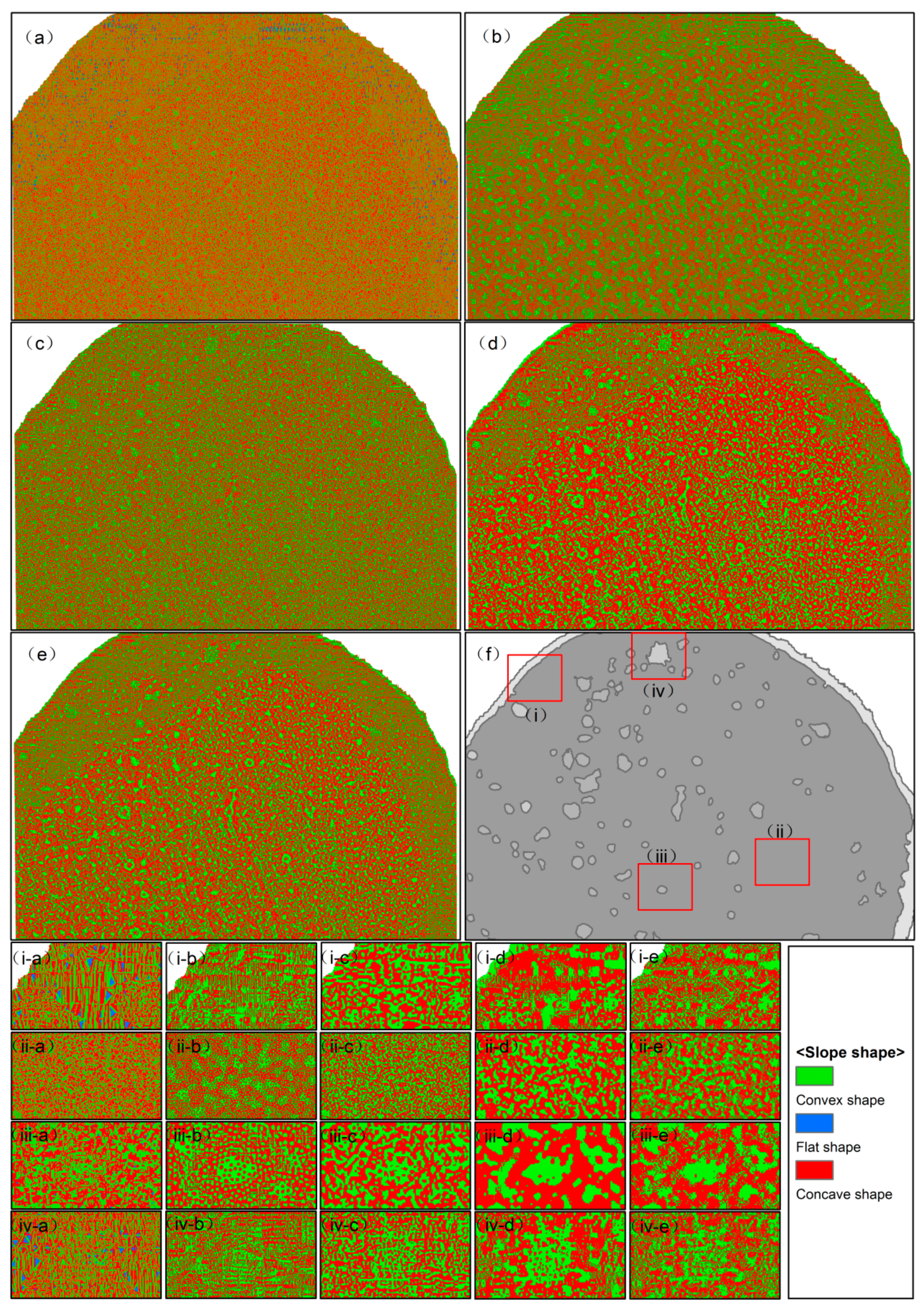
Figure 7.
Slope shape field models of the lagoon. The first slope shape field model was generated from the synthetic surface model from (a) TIN, and the others were generated from the simulated surface models that were reconstructed by (b) IDW, (c) LPI, (d) RBF, and (e) OK. The pattern areas were selected from (f) the lagoon’s geomorphic subunits for further comparison: (i) lagoon slope, (ii) lagoon bottom, (iii) deep patch reef, and (iv) shallow patch reef. The patterns (i-a–iv-e) reflect the differences in the simulated and synthetic surfaces in the slope shape field model.

Figure 8.
Slope aspect field models of the lagoon. The first slope aspect field model was generated from the synthetic surface model from (a) TIN, and the others were generated from the simulated surface models that were reconstructed by (b) IDW, (c) LPI, (d) RBF, and (e) OK. The pattern areas were selected from (f) the lagoon’s geomorphic subunits for further comparison: (i) lagoon slope, (ii) lagoon bottom, (iii) deep patch reef, and (iv) shallow patch reef. The patterns (i-a–iv-e) reflect the differences in the simulated and synthetic surfaces in the slope aspect field model.

Figure 9.
Root mean square error (RMSE) of the surface models with 1-m resolution were reconstructed by (a) IDW, (b) LPI, (c) RBF, and (d) OK: Ze represents the estimated value and Zo represents the observed value.
Figure 9.
Root mean square error (RMSE) of the surface models with 1-m resolution were reconstructed by (a) IDW, (b) LPI, (c) RBF, and (d) OK: Ze represents the estimated value and Zo represents the observed value.

Figure 10.
Change rate of the local slope shape (CRLSS) of the surface models with 1-m resolution were reconstructed by (a) IDW, (b) LPI, (c) RBF, and (d) OK. The six colors in the figure represent the changes among three different local slope shapes, and the size of the shaded area represents the ratio of the changes of different local slope shapes.

Figure 11.
Change rate of the local slope aspect (CRLSA) of the surface models with 1-m resolution were reconstructed by (a) IDW, (b) LPI, (c) RBF, and (d) OK. The eight letters in the figure represent eight different local slope aspects of the synthetic surface model, and the eight different colors represent the eight different local slope aspects of the reconstructed surface model. The size of the color block represents the ratio of each original local slope aspect in the synthetic surface model’s change to the other eight local slope aspects in the reconstructed surface model.

Figure 12.
RMSE of the surface models of different geomorphic subunits: (a) lagoon slope, (b) lagoon bottom, (c) deep patch reef, and (d) shallow patch reef. Ze represents the estimated value and Zo represents the observed value.
Figure 12.
RMSE of the surface models of different geomorphic subunits: (a) lagoon slope, (b) lagoon bottom, (c) deep patch reef, and (d) shallow patch reef. Ze represents the estimated value and Zo represents the observed value.

Figure 13.
CRLSS of the surface models of different geomorphic subunits: (a) lagoon slope, (b) lagoon bottom, (c) deep patch reef, and (d) shallow patch reef. The six colors in the figure represent the changes among the three different local slope shapes, and the size of the shaded area represents the ratio of the changes of different local slope shapes.

Figure 14.
CRLSA of the surface models of different geomorphic subunits: (a) lagoon slope, (b) lagoon bottom, (c) deep patch reef, and (d) shallow patch reef. The eight letters in the figure represent eight different local slope aspects of the synthetic surface model, and the eight different colors represent the eight different local slope aspects of the reconstructed surface model. The size of the color block represents the ratio of changes in each original local slope aspect in the synthetic surface model to the other eight local slope aspects in the reconstructed surface model.


Table 1.
Parameter settings of each interpolation method.
| Interpolation Methods | Interpolation Parameters | ||||
|---|---|---|---|---|---|
| Neighborhood Type | Search Sectors | Search Neighbors | Kernel Function | Function Variable | |
| IDW | Circular | 4 sectors | 10–15 | Power | Power = 2 |
| LPI | Circular | 4 sectors | 10–15 | Gaussian | Order = 1 |
| RBF | Circular | 4 sectors | 10–15 | Multiquadric | Smoothness = 0 |
| OK | Circular | 4 sectors | 10–15 | Spherical | Nugget = 4 |
Table 2.
Performances of the interpolation methods for the morphological surface model reconstructions.
Table 2.
Performances of the interpolation methods for the morphological surface model reconstructions.
| Morphological Precision Indices | Quality Order of the Surface Models that Were Reconstructed by the Interpolation Methods |
|---|---|
| RMSE | OK > RBF > LPI > IDW |
| CRLSS | IDW > LPI > OK > RBF |
| CRLSA | RBF > OK > LPI > IDW |
Table 3.
Mean morphological precision values of the surface models of different geomorphic subunits.
Table 3.
Mean morphological precision values of the surface models of different geomorphic subunits.
| Geomorphology Subunits | Mean Value of the Morphological Precision | ||
|---|---|---|---|
| RMSE | CRLSS | CRLSA | |
| Lagoon slope | 0.3200 | 55.25% | 40.11% |
| Lagoon bottom | 0.3781 | 53.80% | 47.17% |
| Deep patch reef | 0.7769 | 58.07% | 30.11% |
| Shallow patch reef | 0.5553 | 55.78% | 37.38% |
Table 4.
Comprehensive evaluation value of the interpolation methods that were applied to the geomorphic subunits.
Table 4.
Comprehensive evaluation value of the interpolation methods that were applied to the geomorphic subunits.
| Interpolation Methods | Comprehensive Values in the Geomorphic Subunits | |||
|---|---|---|---|---|
| Lagoon Slope (×10−6) | Lagoon Bottom (×10−6) | Deep Patch Reef (×10−3) | Shallow Patch Reef (×10−5) | |
| IDW | 2.89 | 2.39 | 0.12 | 0.75 |
| LPI | 1.55 | 3.11 | 1.10 | 2.46 |
| RBF | 1.81 | 2.92 | 1.43 | 2.31 |
| OK | 1.84 | 2.99 | 1.38 | 2.42 |
Table 5.
Morphological precision of surface models and performance comprehensive evaluation values of interpolation methods when the patch reef was decomposed by the second-order and third-order geomorphic scales.
Table 5.
Morphological precision of surface models and performance comprehensive evaluation values of interpolation methods when the patch reef was decomposed by the second-order and third-order geomorphic scales.
| Geomorphology Units | Interpolation Methods | Morphological Precision | Comprehensive Evaluation Values | |||
|---|---|---|---|---|---|---|
| 2nd-Order | 3rd-Order | RMSE | CRLSS | CRLSA | ||
| Patch reef | IDW | 1.1473 | 54.25% | 37.80% | 0.91 × 10⁻⁴ | |
| LPI | 0.6419 | 54.78% | 31.03% | 7.85 × 10⁻⁴ | ||
| RBF | 0.5876 | 62.29% | 28.47% | 9.91 × 10⁻⁴ | ||
| OK | 0.5939 | 59.29% | 28.39% | 9.65 × 10⁻⁴ | ||
| Deep patch reef | IDW | 1.2237 | 54.50% | 36.77% | 0.12 × 10⁻³ | |
| LPI | 0.6689 | 54.04% | 30.15% | 1.10 × 10⁻³ | ||
| RBF | 0.6031 | 63.51% | 26.83% | 1.43 × 10⁻³ | ||
| OK | 0.6117 | 60.21% | 26.67% | 1.38 × 10⁻³ | ||
| Shallow patch reef | IDW | 0.7034 | 53.10% | 42.48% | 0.75 × 10⁻⁵ | |
| LPI | 0.5011 | 58.15% | 35.02% | 2.46 × 10⁻⁵ | ||
| RBF | 0.5113 | 56.78% | 35.86% | 2.31 × 10⁻⁵ | ||
| OK | 0.5054 | 55.10% | 36.17% | 2.42 × 10⁻⁵ | ||
© 2018 by the authors. Licensee MDPI, Basel, Switzerland. This article is an open access article distributed under the terms and conditions of the Creative Commons Attribution (CC BY) license (http://creativecommons.org/licenses/by/4.0/).
Share and Cite
MDPI and ACS Style
Wang, Q.; Su, F.; Zhang, Y.; Jiang, H.; Cheng, F. Morphological Precision Assessment of Reconstructed Surface Models for a Coral Atoll Lagoon. Sustainability 2018, 10, 2749. https://doi.org/10.3390/su10082749
AMA Style
Wang Q, Su F, Zhang Y, Jiang H, Cheng F. Morphological Precision Assessment of Reconstructed Surface Models for a Coral Atoll Lagoon. Sustainability. 2018; 10(8):2749. https://doi.org/10.3390/su10082749
Chicago/Turabian StyleWang, Qi, Fenzhen Su, Yu Zhang, Huiping Jiang, and Fei Cheng. 2018. "Morphological Precision Assessment of Reconstructed Surface Models for a Coral Atoll Lagoon" Sustainability 10, no. 8: 2749. https://doi.org/10.3390/su10082749
Note that from the first issue of 2016, this journal uses article numbers instead of page numbers. See further details here.