Soil Salinity Mapping of Urban Greenery Using Remote Sensing and Proximal Sensing Techniques; The Case of Veale Gardens within the Adelaide Parklands

 , ,
, ,  , and
, and
Abstract
:1. Introduction
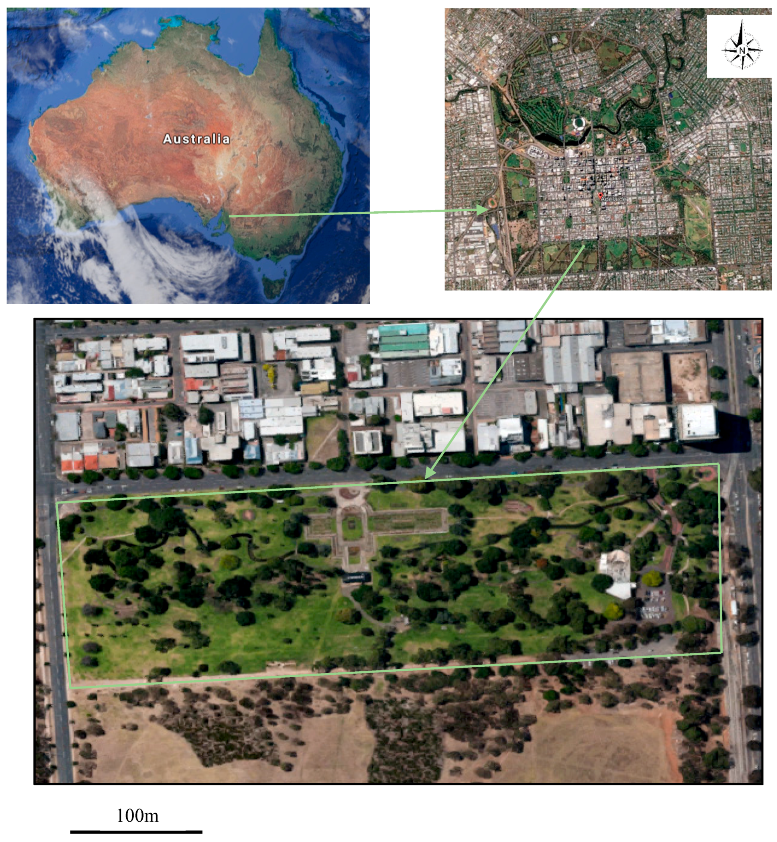
2. Study Area
3. Material and Methods
3.1. Proximal Sensing and Laboratory
3.2. Optical Remote Sensing
3.3. Modeling Soil Salinity Using Proximal and Remote Sensing Data
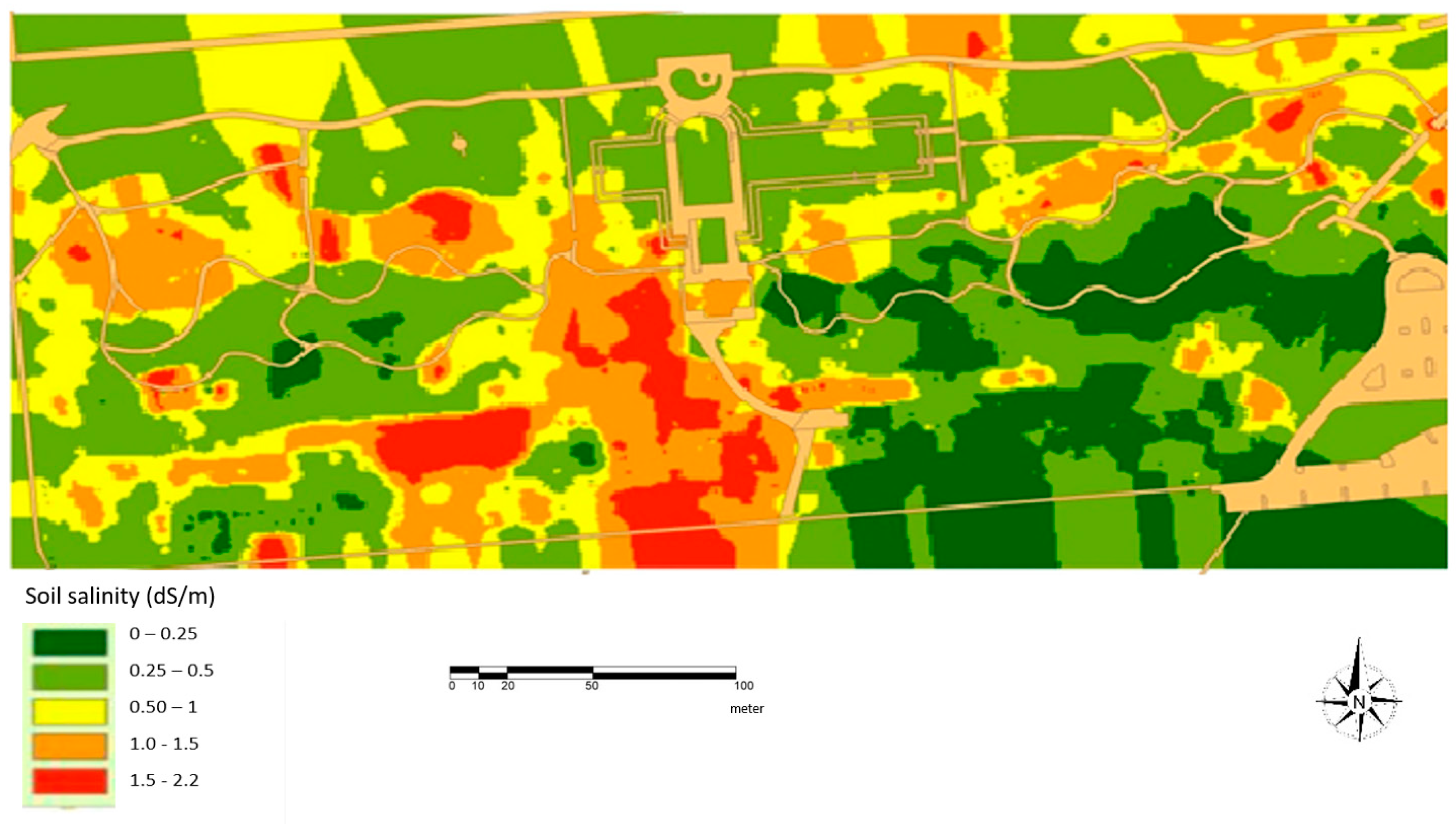
4. Results and Discussion
4.1. Proximal Sensing and Laboratory
4.2. Optical Remote Sensing
4.3. Modeling Soil Salinity Using Near and Remote Sensing Data
5. Conclusions and Recommendations
Author Contributions
Funding
Acknowledgments
Conflicts of Interest
References
- Nouri, H.; Beecham, S.; Hassanli, A.M.; Ingleton, G. Variability of drainage and solute leaching in heterogeneous urban vegetation environs. Hydrol. Earth Syst. Sci. 2013, 17, 4339–4347. [Google Scholar] [CrossRef] [Green Version]
- Aimrun, W.; Amin, M.S.M.; Nouri, H. Paddy Field Zone Characterization using Apparent Electrical Conductivity for Rice Precision Farming. Int. J. Agric. Res. 2011, 1, 10–28. [Google Scholar] [CrossRef]
- Scudiero, E.; Corwin, D.L.; Morari, F.; Anderson, R.G.; Skaggs, T.H. Spatial interpolation quality assessment for soil sensor transect datasets. Comput. Electron. Agric. 2016, 123, 74–79. [Google Scholar] [CrossRef]
- Saleh, A.A.-H. Remote Sensing of Soil Salinity in an Arid Areas in Saudi Arabia. Int. J. Civ. Environ. Eng. 2010, 10, 12–17. [Google Scholar]
- Alizade Govarchin Ghale, Y.; Baykara, M.; Unal, A. Analysis of decadal land cover changes and salinization in Urmia Lake Basin using remote sensing techniques. Nat. Hazards Earth Syst. Sci. Discuss. 2017, 2017, 1–15. [Google Scholar] [CrossRef]
- Khan, N.M.; Rastoskuev, V.V.; Shalina, E.V.; Sato, Y. Mapping salt-affected soils using remote sensing indicators-A simple approach with the use of GIS IDRIS. In Proceedings of the 22nd Asian Conference on Remote Sensing, Singapore, 5–9 November 2001. [Google Scholar]
- Whitney, K.; Scudiero, E.; El-Askary, H.M.; Skaggs, T.H.; Allali, M.; Corwin, D.L. Validating the use of MODIS time series for salinity assessment over agricultural soils in California, USA. Ecol. Indic. 2018, 93, 889–898. [Google Scholar] [CrossRef]
- Dehni, A.; Lounis, M. Remote Sensing Techniques for Salt Affected Soil Mapping: Application to the Oran Region of Algeria. Procedia Eng. 2012, 33, 188–198. [Google Scholar] [CrossRef]
- Alexakis, D.D.; Daliakopoulos, I.N.; Panagea, I.S.; Tsanis, I.K. Assessing soil salinity using WorldView-2 multispectral images in Timpaki, Crete, Greece. Geocarto Int. 2018, 33, 321–338. [Google Scholar] [CrossRef]
- Long, M. A Biodiversity Survey of the Adelaide Park Lands, South Australia in 2003; Department for Environment and Heritage: Adelaide, South Australia, Australia, 2003.
- Metternicht, G.; Zinck, A. Remote Sensing of Soil Salinization: Impact on Land Management; CRC Press: Boca Raton, FL, USA, 2008. [Google Scholar]
- Hengl, T. A Practical Guide to Geostatistical Mapping of Environmental Variables; Institute for Environment and Sustainability, European Commission-Joint Research Centre: Ispra, Italy, 2007. [Google Scholar]
- Ding, J.; Yu, D. Monitoring and evaluating spatial variability of soil salinity in dry and wet seasons in the Werigan–Kuqa Oasis, China, using remote sensing and electromagnetic induction instruments. Geoderma 2014, 235–236, 316–322. [Google Scholar] [CrossRef]
- Heil, K.; Schmidhalter, U. Comparison of the EM38 and EM38-MK2 electromagnetic induction-based sensors for spatial soil analysis at field scale. Comput. Electron. Agric. 2015, 110, 267–280. [Google Scholar] [CrossRef]
- Li, H.Y.; Shi, Z.; Webster, R.; Triantafilis, J. Mapping the three-dimensional variation of soil salinity in a rice-paddy soil. Geoderma 2013, 195–196, 31–41. [Google Scholar] [CrossRef]
- Lesch, S.M.; Rhoades, J.D.; Herrero, J. Monitoring for Temporal Changes in Soil Salinity using Electromagnetic Induction Techniques. Soil Sci. Soc. Am. J. 1998, 62, 232–242. [Google Scholar] [CrossRef] [Green Version]
- Li, X.-M.; Yang, J.-S.; Liu, M.-X.; Liu, G.-M.; Yu, M. Spatio-Temporal Changes of Soil Salinity in Arid Areas of South Xinjiang Using Electromagnetic Induction. J. Integr. Agric. 2012, 11, 1365–1376. [Google Scholar] [CrossRef]
- Yao, R.; Yang, J. Quantitative evaluation of soil salinity and its spatial distribution using electromagnetic induction method. Agric. Water Manag. 2010, 97, 1961–1970. [Google Scholar] [CrossRef]
- Zheng, Z.; Zhang, F.R.; Ma, F.Y.; Chai, X.R.; Zhu, Z.Q.; Shi, J.L.; Zhang, S.X. Spatiotemporal changes in soil salinity in a drip-irrigated field. Geoderma 2009, 149, 243–248. [Google Scholar] [CrossRef]
- Brevik, E.; Fenton, T.; Lazari, A. Soil electrical conductivity as a function of soil water content and implications for soil mapping. Precis. Agric 2006, 7, 393–404. [Google Scholar] [CrossRef]
- Geonics Limited. EM38 Ground Conductivity Meter Operating Manual; Geonics Limited: Mississauga, ON, Canada, 2002. [Google Scholar]
- Doolittle, J.A.; Brevik, E.C. The use of electromagnetic induction techniques in soils studies. Geoderma 2014, 223–225, 33–45. [Google Scholar] [CrossRef]
- Scudiero, E.; Skaggs, T.H.; Corwin, D.L. Regional-scale soil salinity assessment using Landsat ETM + canopy reflectance. Remote. Sens. Environ. 2015, 169, 335–343. [Google Scholar] [CrossRef] [Green Version]
- Brevik, E.C. Analysis of the Representation of Soil Map Units using a Common Apparent Electrical Conductivity Sampling Design for the Mapping of Soil Properties. Soil Horiz. 2012, 53, 32–37. [Google Scholar] [CrossRef]
- Bhunia, G.S.; Shit, P.K.; Maiti, R. Comparison of GIS-based interpolation methods for spatial distribution of soil organic carbon (SOC). J. Saudi Soc. Agric. Sci. 2016. [Google Scholar] [CrossRef]
- Gong, G.; Mattevada, S.; O’Bryant, S.E. Comparison of the accuracy of kriging and IDW interpolations in estimating groundwater arsenic concentrations in Texas. Environ. Res. 2014, 130, 59–69. [Google Scholar] [CrossRef] [PubMed]
- Xie, Y.; Chen, T.-B.; Lei, M.; Yang, J.; Guo, Q.-J.; Song, B.; Zhou, X.-Y. Spatial distribution of soil heavy metal pollution estimated by different interpolation methods: Accuracy and uncertainty analysis. Chemosphere 2011, 82, 468–476. [Google Scholar] [CrossRef] [PubMed]
- Zhu, Q.; Lin, H.S. Comparing Ordinary Kriging and Regression Kriging for Soil Properties in Contrasting Landscapes. Pedosphere 2010, 20, 594–606. [Google Scholar] [CrossRef]
- Cook, R.A.; Mostaghimi, S.; Campbell, J.B. Assessment of methods for interpolating steady-state infiltration. Trans. ASAE 1993, 36, 1241–1333. [Google Scholar]
- Gumiere, S.J.; Lafond, J.A.; Hallema, D.W.; Périard, Y.; Caron, J.; Gallichand, J. Mapping soil hydraulic conductivity and matric potential for water management of cranberry: Characterisation and spatial interpolation methods. Biosyst. Eng. 2014, 128, 29–40. [Google Scholar] [CrossRef]
- Neely, H.L.; Morgan, C.L.S.; Hallmark, C.T.; McInnes, K.J.; Molling, C.C. Apparent electrical conductivity response to spatially variable vertisol properties. Geoderma 2016, 263, 168–175. [Google Scholar] [CrossRef] [Green Version]
- Piikki, K.; Söderström, M.; Stenberg, B. Sensor data fusion for topsoil clay mapping. Geoderma 2013, 199, 106–116. [Google Scholar] [CrossRef]
- Rodrigues, F.A.; Bramley, R.G.V.; Gobbett, D.L. Proximal soil sensing for Precision Agriculture: Simultaneous use of electromagnetic induction and gamma radiometrics in contrasting soils. Geoderma 2015, 243–244, 183–195. [Google Scholar] [CrossRef]
- Anderson, S. An Evaluation of Spatial Interpolation Methods on Air Temperature in Phoenix, AZ. 2002. Available online: http://www.cobblestoneconcepts.com/ucgis2summer/anderson/anderson.htm (accessed on 15 February 2016).
- Eldeiry, A.; García, L. Using Deterministic and Geostatistical Techniques to Estimate Soil Salinity at the Sub-Basin Scale and the Field Scale. In Proceedings of the 31th Annual Hydrology Days, Fort Collins, CO, USA, 21–23 March 2011. [Google Scholar]
- Urquhart, E.A.; Hoffman, M.J.; Murphy, R.R.; Zaitchik, B.F. Geospatial interpolation of MODIS-derived salinity and temperature in the Chesapeake Bay. Remote. Sens. Environ. 2013, 135, 167–177. [Google Scholar] [CrossRef]
- Allbed, A.; Kumar, L. Soil Salinity Mapping and Monitoring in Arid and Semi-Arid Regions Using Remote Sensing Technology: A Review. Adv. Remote Sens. 2013, 2, 373. [Google Scholar] [CrossRef]
- Asadzadeh, S.; de Souza Filho, C.R. Investigating the capability of WorldView-3 superspectral data for direct hydrocarbon detection. Remote Sens. Environ. 2016, 173, 162–173. [Google Scholar] [CrossRef]
- Gorji, T.; Tanik, A.; Sertel, E. Soil Salinity Prediction, Monitoring and Mapping Using Modern Technologies. Procedia Earth Planet. Sci. 2015, 15, 507–512. [Google Scholar] [CrossRef]
- Metternicht, G.I.; Zinck, J.A. Remote sensing of soil salinity: Potentials and constraints. Remote Sens. Environ. 2003, 85, 1–20. [Google Scholar] [CrossRef]
- Pu, R.; Landry, S. A comparative analysis of high spatial resolution IKONOS and WorldView-2 imagery for mapping urban tree species. Remote Sens. Environ. 2012, 124, 516–533. [Google Scholar] [CrossRef]
- Kruse, F.A.; Baugh, W.M.; Perry, S.L. Validation of DigitalGlobe WorldView-3 Earth imaging satellite shortwave infrared bands for mineral mapping. J. Appl. Remote Sens. 2015, 9, 096044. [Google Scholar] [CrossRef]
- Taylor, G.R.; Mah, A.H.; Kruse, F.A.; Kierein-Young, K.S.; Hewson, R.D.; Bennett, B.A. Characterization of saline soils using airborne radar imagery. Remote Sens. Environ. 1996, 57, 127–142. [Google Scholar] [CrossRef]
- Nouri, H.; Greg, I.; Beecham, S.; Anderson, S. Remotely-Sensed Modelling of Soil Salinity from WasteWater Irrigation in the Adelaide Parklands; SA Water: Adelaide, South Australia, Australia, 2016. [Google Scholar]
- Rouse, J.W.; Hass, R.H.; Schell, J.A.; Deering, D.W. Monitoring vegetation systems in the Great Plains with ERTS. In Proceedings of the Third ERTS Symposium, Washington, DC, USA, 10–14 December 1973; pp. 309–317. [Google Scholar]
- Liu, H.Q.; Huete, A.R. A feedback based modification of the NDV I to minimize canopy background and atmospheric noise. IEEE Trans. Geosci. Remote Sens. 1995, 33, 457–465. [Google Scholar]
- Huete, A.R. A soil-adjusted vegetation index (SAVI). Remote. Sens. Environ. 1988, 25, 295–309. [Google Scholar] [CrossRef]
- Pearson, R.L.; Miller, L.D. Remote mapping of standing crop biomass for estimation of the productivity of the short-grass Prairie, Pawnee National Grasslands Colorado. In Proceedings of the Eighth International Symposium on Remote Sensing of Environment, Ann Arbor, MI, USA, 2–6 October 1976; Willow Run Laboratories, Environmental Research Institute of Michigan: Ann Arbor, MI, USA, 1972; pp. 1357–1381. [Google Scholar]
- Tripathi, N.K.; Rai, B.K.; Dwivedi, P. Spatial Modeling of Soil Alkalinity in GIS Environment Using IRS data. In Proceedings of the 18th Asian Conference on Remote Sensing, Kuala Lumpur, Malaysia, 20–25 October 1997; pp. A.8.1–A.8.6. [Google Scholar]
- Khan, N.M.; Rastoskuev, V.V.; Sato, Y.; Shiozawa, S. Assessment of hydrosaline land degradation by using a simple approach of remote sensing indicators. Agric. Water Manag. 2005, 77, 96–109. [Google Scholar] [CrossRef]
- Douaoui, A.E.K.; Nicolas, H.; Walter, C. Detecting salinity hazards within a semiarid context by means of combining soil and remote-sensing data. Geoderma 2006, 134, 217–230. [Google Scholar] [CrossRef]
- IDNP. Indo-Dutch Network Project: A Methodology for Identification of Waterlogging and Soil Salinity Conditions Using Remote Sensing; IDNP: Karnal, India, 2003. [Google Scholar]
- Bannari, A.; Guedon, A.M.; El-Harti, A.; Cherkaoui, F.Z.; El-Ghmari, A. Characterization of Slightly and Moderately Saline and Sodic Soils in Irrigated Agricultural Land using Simulated Data of Advanced Land Imaging (EO-1) Sensor. Commun. Soil Sci. Plant Anal. 2008, 39, 2795–2811. [Google Scholar] [CrossRef]
- Abbas, A.; Khan, S. Using Remote Sensing Techniques for Appraisal of Irrigated Soil Salinity. In Proceedings of the International Congress on Modelling and Simulation (MODSIM), Christchurch, New Zealand, 10–13 December 2007; pp. 2632–2638. Available online: https://www.mssanz.org.au/MODSIM07/papers/46_s60/UsingRemotes60_Abbas_.pdf (accessed on 4 April 2018).
- Noureddine, K.; Eddine, M.D.; Kader, D.A.E. New Index for Salinity Assessment Applied on Saline Context Area (Case of the Lower Chiff Plain). Int. J. Sci. Basic Appl. Res. 2014, 18, 401–404. [Google Scholar]
- Baret, F.; Guyot, G.; Major, D.J. TSAVI: A vegetation index which minimizes soil brightness effects on LAI and APAR estimation. In Proceedings of the Geoscience and Remote Sensing Symposium-IGARSS’89/12th International Canadian Symposium on Remote Sensing, Vancouver, BC, Canada, 10–14 July 1989; IEEE: New York, NY, USA, 1989; pp. 1355–1358. [Google Scholar]
- Bouaziz, M.; Matschullat, J.; Gloaguen, R. Improved remote sensing detection of soil salinity from a semi-arid climate in Northeast Brazil. C. R. Geosci. 2011, 343, 795–803. [Google Scholar] [CrossRef]
- Basso, F.; Bove, E.; Dumontet, S.; Ferrara, A.; Pisante, M.; Quaranta, G.; Taberner, M. Evaluating environmental sensitivity at the basin scale through the use of geographic information systems and remotely sensed data: An example covering the Agri basin (Southern Italy). Catena 2000, 40, 19–35. [Google Scholar] [CrossRef]
- Ekercin, S.; Ormeci, C. Estimating Soil Salinity Using Satellite Remote Sensing Data and Real-Time Field Sampling. Environ. Eng. Sci. 2008, 25, 981–988. [Google Scholar] [CrossRef]
- Yu, C.; Fu, C.; Huo, L.Q. The feasibility study of soil moisture monitoring based on MODIS data under different vegetation coverage. J. Remote Sens. 2006, 10, 783–788. [Google Scholar]
- Zarco-Tejada, P.J.; Rueda, C.A.; Ustin, S.L. Water content estimation in vegetation with MODIS reflectance data and model inversion methods. Remote Sensing of Environment. Remote Sens. Environ. 2003, 85, 109–124. [Google Scholar] [CrossRef]
- Lovejoy, S.; Schertzer, D.; Allaire, V.C. The remarkable wide range spatial scaling of TRMM precipitation. Atmos. Res. 2008, 90, 10–32. [Google Scholar] [CrossRef]
- Stow, D.; Niphadkar, M.; Kaiser, J. MODIS-derived visible atmospherically resistant index for monitoring chaparral moisture content. Int. J. Remote Sens. 2005, 26, 3867–3873. [Google Scholar] [CrossRef]
- Hardisky, M.A.; Klemas, V.; Smart, R.M. The influence of soil salinity, growth form, and leaf moisture on the spectral radiance of spartinaalterniora canopies. Hotogramm. Eng. Remote Sens. 1983, 49, 77–83. [Google Scholar]
- Karnieli, A.; Kaufman, Y.J.; Remer, L.; Wald, A. AFRI—Aerosol free vegetation index. Remote Sens. Environ. 2001, 77, 10–21. [Google Scholar] [CrossRef]
- Xiao, X.; Zhang, Q.; Saleska, S.; Hutyra, L.; De Camargo, P.; Wofsy, S.; Frolking, S.; Boles, S.; Keller, M.; Moore, B. Satellite-based modeling of gross primary production in a seasonally moist tropical evergreen forest. Remote Sens. Environ. 2005, 94, 105–122. [Google Scholar] [CrossRef]
- Wang, L.; Qu, J. NMDI: A normalized multi-band drought index for monitoring soil and vegetation moisture with satellite remote sensing. Geophys. Res. Lett. 2007, 34. [Google Scholar] [CrossRef] [Green Version]
- Nield, S.J.; Boettinger, J.L.; Ramsey, R.D. Digitally Mapping Gypsic and Natric Soil Areas Using Landsat ETM Data Abbreviations: DEM, digital elevation model; NDVI, normalized difference vegetation index; NIR, near infrared; OIF, optimum index factor; SWIR, shortwave infrared. Soil Sci. Soc. Am. J. 2007, 71, 245–252. [Google Scholar] [CrossRef]
- Ding, J.-L.; Wu, M.-C.; Tiyip, T. Study on Soil Salinization Information in Arid Region Using Remote Sensing Technique. Agric. Sci. China 2011, 10, 404–411. [Google Scholar] [CrossRef]
- Abrol, P.; Yadav, J.S.P.; Massoud, F.I. Salt-Affected Soils and Their Management; FAO Soil Resources Management and Conservation Service: Rome, Italy, 1998. [Google Scholar]


| Indices | Equation | Ref. | |
|---|---|---|---|
| 1 | Normalized Differential Vegetation Index | [45] | |
| 2 | Enhanced Vegetation Index | [46] | |
| 3 | Soil Adjusted Vegetation Index | [47] | |
| 4 | Ratio Vegetation Index | [48] | |
| 5 | Normalized Differential Salinity Index | [49] | |
| 6 | Brightness Index | [50] | |
| 7 | Salinity Index | [49] | |
| 8 | Salinity Index | [50] | |
| 9 | Salinity Index | [51] | |
| 10 | Salinity Index | [51] | |
| 11 | Salinity Index | B5/B7 | [52] |
| 12 | Salinity Index | [52] | |
| 13 | Salinity Index | [53] | |
| 14 | Soil Salinity and Sodicity Indices | SSSI-1 = (B5 − B7) | [53] |
| 15 | Soil Salinity and Sodicity Indices | SSSI-2 = (B5 × B7 − B7 × B7)/B5 | [53] |
| 16 | Salinity Index | S1 = B1/B3 | [53] |
| 17 | Salinity Index | S2 = (B1 − B3)/(B1 + B3) | [53] |
| 18 | Salinity Index | S3 = (B2 × B3)/B1 | [53] |
| 19 | Salinity Index | S5 = (B1 × B3)/B2 | [54] |
| 20 | Salinity Index | S6 = (B2 × B4)/B2 | [54] |
| 21 | Salinity Index | ) | [55] |
| 22 | Salinity Index | [56] | |
| 23 | Perpendicular Vegetation Index | [56] | |
| 24 | Salinity Index | [57] | |
| 25 | Salinity Index | [57] | |
| 26 | Salinity Index | [58] | |
| 27 | Salinity Index | [58] | |
| 28 | Salinity Index | [57] | |
| 29 | Salinity Index | [59] | |
| 30 | Salinity Index | [57] | |
| 31 | Normalized Difference Water Index | [60] | |
| 32 | Simple Ratio Water Index | [61] | |
| 33 | Soil Surface Moisture | [62] | |
| 34 | Visible Atmospherically Resistant Index | [63] | |
| 35 | Normalized Difference Infrared Index | [64] | |
| 36 | Aerosol-free Vegetation Index | AFRI1.6 = | [65] |
| 37 | Aerosol-free Vegetation Index | AFRI2.1 = | [65] |
| 38 | Land Surface Water Index | LSWI = (NIR − SWIR)/(NIR + SWIR) | [66] |
| 39 | Normalized Multi-band Drought Index | [67] | |
| 40 | Gypsic Index | [68] | |
| 41 | Similarly Index | [68] | |
| 42 | Salinity Index | [69] | |
| 43 | Salinity Index | SI-1(2) = | [20] |
| 44 | Salinity Index | SI-2(2) = | [20] |
| 45 | Salinity Index | SI-3(2) = | [20] |
| Mean | Median | Maximum | Minimum | SD-P | SD-S | CV (%) |
|---|---|---|---|---|---|---|
| 0.537 | 0.413 | 2.130 | 0.203 | 0.402 | 0.411 | 0.748 |
| OBJECT_ID | 1 | 2 | 3 | 4 | 5 |
|---|---|---|---|---|---|
| EM38 | 22.1 | 21.9 | 20.9 | 19.9 | 20.4 |
| NDSI (R-NIR)/(R + NIR) | −0.677 | −0.677 | −0.677 | −0.656 | −0.656 |
| NDVI | 0.677 | 0.677 | 0.677 | 0.656 | 0.656 |
| EVI 2.5(NIR-red)/(NIR + 6red-7.5 blue + 1) | −3.08 | −3.08 | −3.08 | −3.198 | −3.198 |
| SAVI (NIR-R)/(NIR + R + L) (1 + L) | 0.501 | 0.501 | 0.501 | 0.485 | 0.485 |
| RVI (NIR/R) | 5.193 | 5.193 | 5.193 | 4.806 | 4.806 |
| BI (R2 + NIR2)1/2 | 602.876 | 602.876 | 602.876 | 608.763 | 608.763 |
| SI (blue × red)1/2 | 159.085 | 159.085 | 159.085 | 168.143 | 168.143 |
| SII (green × red)1/2 | 167.463 | 167.463 | 167.463 | 178.863 | 178.863 |
| SI2 (G2 + R2 + NIR2)1/2 | 651.134 | 651.134 | 651.134 | 661.178 | 661.178 |
| SI3 (G2 + R2)1/2 | 271.131 | 271.131 | 271.131 | 286.252 | 286.252 |
| S1 (blue/red) | 1.947 | 1.947 | 1.947 | 1.839 | 1.839 |
| S2 (blue-red)/(blue + red) | 0.321 | 0.321 | 0.321 | 0.295 | 0.295 |
| S3 (G × red)/blue | 126.324 | 126.324 | 126.324 | 140.316 | 140.316 |
| S4 (blue × red)1/2 | 102.878 | 102.878 | 102.878 | 109.581 | 109.581 |
| S5 (blue × red)/green | 102.878 | 102.878 | 102.878 | 109.581 | 109.581 |
| S6 (red × NIR)/green | 274.341 | 274.341 | 274.341 | 286.45 | 286.45 |
| DVI1 (NIR1-red) | 478 | 478 | 478 | 472 | 472 |
| DVI2 (NIR2-red) | 292 | 292 | 292 | 287 | 287 |
| DVI3 (NIR1-redEdge) | 286 | 286 | 286 | 283 | 283 |
| DVI4 (NIR2-redEdge) | 100 | 100 | 100 | 98 | 98 |
| GDVI1 (NIR1-green) | 346 | 346 | 346 | 338 | 338 |
| GDVI2 (NIR2-green) | 160 | 160 | 160 | 153 | 153 |
| EM38 | B1 Coastal | B2 Blue | B3 Green | B4 Yellow | B5 Red | B6 Red-Edge | B7 NIR1 | B8 NIR2 | |
|---|---|---|---|---|---|---|---|---|---|
| EM38 | 1 | ||||||||
| B1Coastal | 0.0559 | 1 | |||||||
| B2Blue | 0.0792 | 0.9463 | 1 | ||||||
| B3Green | 0.1043 | 0.8284 | 0.9163 | 1 | |||||
| B4Yellow | 0.0865 | 0.8783 | 0.9467 | 0.9636 | 1 | ||||
| B5Red | 0.0607 | 0.8891 | 0.9555 | 0.9040 | 0.9647 | 1 | |||
| B6Red-Edge | 0.0995 | 0.5384 | 0.6426 | 0.8576 | 0.7839 | 0.6508 | 1 | ||
| B7NIR1 | 0.084 | 0.3899 | 0.4807 | 0.7327 | 0.6067 | 0.4595 | 0.9445 | 1 | |
| B8NIR2 | 0.0805 | 0.3968 | 0.4911 | 0.737 | 0.6216 | 0.4728 | 0.9517 | 0.9797 | 1 |
| EM38 | Coef. | P > z |
|---|---|---|
| B1 (Coastal Blue) | −0.07353 | 0.009 |
| B6 (Red-Edge) | 0.09696 | 0 |
| B7 (NIR1) | −0.02300 | 0 |
| _cons | 98.99310 | 0 |
| AIC | 573,957.7 | |
| BIC | 574,002 |
| Model 2 | Model 3 | Model 4 | Model 5 | Model 6 | Model 7 | |||||||
|---|---|---|---|---|---|---|---|---|---|---|---|---|
| EM38v | Coef. | P > z | Coef. | P > z | Coef. | P > z | Coef. | P > z | Coef. | P > z | Coef. | P > z |
| B1 (Coastal Blue) | 0.6 | 0.283 | −0.3398 | 0.000 | 0.09947 | 0.062 | −0.3358 | 0 | −0.1099 | 0.021 | ||
| B6 (Red-Edge) | 0.11027 | 0.000 | 0.06795 | 0.000 | 0.14895 | 0.000 | 0.04417 | 0 | ||||
| B7 (NIR1) | −0.0182 | 0.000 | 0.00882 | 0.000 | −0.0053 | 0.09 | 0.00714 | 0 | ||||
| B3 (Green) | 0.05588 | 0.000 | 0.06524 | 0 | ||||||||
| B4 (Yellow) | −0.0771 | 0.000 | −0.1078 | 0.000 | 0.25464 | 0.000 | 0.31922 | 0 | ||||
| B8 (NIR2) | −0.0207 | 0.000 | −0.047 | 0.000 | ||||||||
| B5 (Red) | −0.3262 | 0.000 | −0.2625 | 0 | ||||||||
| B2 (Blue) | 0.18741 | 0.000 | ||||||||||
| _cons | 82.1058 | 0.000 | 137.835 | 0.000 | 76.4472 | 0.000 | 53.2329 | 0.000 | 136.2 | 0 | 99.3143 | 0 |
| AIC | 568,774 | 568,749 | 568,732 | 568,668 | 568,764 | 568,708 | ||||||
| BIC | 568,836 | 568,811 | 568,794 | 568,731 | 568,826 | 568,770 | ||||||
| Model 8 | Model 9 | Model 10 | Model 11 | Model 12 | Model 13 | |||||||
|---|---|---|---|---|---|---|---|---|---|---|---|---|
| EM38v | Coef. | P > z | Coef. | P > z | Coef. | P > z | Coef. | P > z | Coef. | P > z | Coef. | P > z |
| B1 (Coastal Blue) | 0.059 | 0.009 | −0.107 | 0.000 | −0.115 | 0.000 | 0.039 | 0.078 | −0.039 | 0.046 | ||
| B6 (Red-Edge) | 0.055 | 0.000 | 0.028 | 0.000 | 0.025 | 0.000 | 0.055 | 0.000 | ||||
| B7 (NIR1) | −0.021 | 0.000 | −0.014 | −0.007 | 0.000 | −0.007 | 0.000 | |||||
| B3 (Green) | 0.023 | 0.000 | 0.026 | 0.000 | ||||||||
| B4 (Yellow) | −0.037 | 0.000 | −0.031 | 0.000 | 0.139 | 0.000 | 0.134 | 0.000 | ||||
| B8 (NIR2) | −0.022 | 0.000 | 0.000 | −0.030 | 0.000 | |||||||
| B5 (Red) | −0.107 | 0.000 | −0.109 | 0.000 | ||||||||
| B2 (Blue) | −0.005 | 0.694 | ||||||||||
| _cons | 120.474 | 0.003 | 143.394 | 0.000 | 144.611 | 0.000 | 123.262 | 0.002 | 131.745 | 0.001 | 126.268 | 0.002 |
| AIC | 478,380 | 478,386 | 478,378 | 478,387 | 478,362 | 478,366 | ||||||
| BIC | 478,442 | 478,448 | 478,440 | 478,450 | 478,424 | 478,428 | ||||||
| EM38 | Coef. | Std. Err. | z P > z | [95% Conf. | Interval] |
|---|---|---|---|---|---|
| EVI | 0.0004198 | 0.001419 | 0.30 0.767 | −0.00236 | 0.003202 |
| SAVI | 45.82032 | 2.641757 | 17.34 0.000 | 40.64257 | 50.99807 |
| _cons | 83.14401 | 5.576818 | 14.91 0.000 | 72.21364 | 94.07437 |
© 2018 by the authors. Licensee MDPI, Basel, Switzerland. This article is an open access article distributed under the terms and conditions of the Creative Commons Attribution (CC BY) license (http://creativecommons.org/licenses/by/4.0/).
Share and Cite
Nouri, H.; Chavoshi Borujeni, S.; Alaghmand, S.; Anderson, S.J.; Sutton, P.C.; Parvazian, S.; Beecham, S. Soil Salinity Mapping of Urban Greenery Using Remote Sensing and Proximal Sensing Techniques; The Case of Veale Gardens within the Adelaide Parklands. Sustainability 2018, 10, 2826. https://doi.org/10.3390/su10082826
Nouri H, Chavoshi Borujeni S, Alaghmand S, Anderson SJ, Sutton PC, Parvazian S, Beecham S. Soil Salinity Mapping of Urban Greenery Using Remote Sensing and Proximal Sensing Techniques; The Case of Veale Gardens within the Adelaide Parklands. Sustainability. 2018; 10(8):2826. https://doi.org/10.3390/su10082826
Chicago/Turabian StyleNouri, Hamideh, Sattar Chavoshi Borujeni, Sina Alaghmand, Sharolyn J. Anderson, Paul C. Sutton, Somayeh Parvazian, and Simon Beecham. 2018. "Soil Salinity Mapping of Urban Greenery Using Remote Sensing and Proximal Sensing Techniques; The Case of Veale Gardens within the Adelaide Parklands" Sustainability 10, no. 8: 2826. https://doi.org/10.3390/su10082826