Abstract
This study was undertaken to forecast the waste generation rates of the accommodation sector in North Cyprus. Three predictor models, multiple linear regression (MLR), artificial neural networks (ANNs) and central composite design (CCD), were applied to predict the waste generation rate during the lean and peak seasons. ANN showed highest prediction performance, specifically, lowest values of the standard error of prediction (SEP = 2.153), mean absolute error (MAE = 1.378) and highest R2 value (0.998) confirmed the accuracy of the model. The analysed waste was categorised into recyclable, general waste and food residue. The authors estimated the total waste generated during the lean season at 2010.5 kg/day, in which large hotels accounted for the largest fraction (66.7%), followed by medium-sized hotels (19.4%) and guesthouses (2.6%). During the peak season, about 49.6% increases in waste generation rates were obtained. Interestingly, 45% of the waste was generated by British tourists, while the least waste was generated by African tourists (7.5%). The ANN predicted that small and large hotels would produce 5.45 and 22.24 tons of waste by the year 2020, respectively. The findings herein are promising and useful in establishing a sustainable waste management system.
1. Introduction
In recent decades, tourism has become one of the most important and significant sectors in the economies of many countries. In fact, the sector accounts for 10–12% of the world’s Gross Domestic Product (GDP) and approximately 14% of total employment [1]. Even though tourism can sustain high levels of employment, the sector is a source of environmental impacts with consequent public health concerns [2]. One of the most significant impacts of tourism is the generation of municipal waste, which increases as the seasonal population of tourists rises [3,4]. The heterogeneous nature of hospitality waste poses a significant risk to water and air quality, and is generally liable to cause various health hazards if not properly managed.
From a sustainability perspective, one approach to the reduction of the threatening environmental and health impacts from hospitality generated wastes is the conversion to useful value-added or alternative products. In this regard, several governments have launched policies to promote the conversion of municipal waste to green precursors or products, many with a specific focus on green fertilizers, bioelectricity, biofuels or bioadsorbents [5,6,7,8,9].
However, to manage and reutilize hospitality sector waste (HSW) in a sustainable way, accurate prediction of HSW generation rate and composition is important [10,11,12]. A failure to make accurate HSW predictions and assessments could lead to several widespread problems in waste management systems and the environment, including irrelevant policies, increased environmental impacts as well as inadequate or overestimated capacity of disposal infrastructures. Inefficient disposal or waste management infrastructure can cause serious impacts on health [1,4]. Specifically, improperly managed, designed and operated recycling/incineration plants cause air pollution or spread of disease. For instance, hotel kitchen waste ferments after a short time, creating conditions favourable to the growth and survival of microbial pathogens and resulting in the spread of infectious diseases. Also, spent cooking oil is a common hospitality waste; note that unattended spent cooking oil attracts flies, vermin and rats, which could create a health hazard and pest control problem.
Cyprus, politically partitioned into two main parts (south and north), is a major tourist destination in the Mediterranean region. Comparatively speaking, recent years have seen tourism growing at a faster rate in North Cyprus (formally the Turkish Republic of North Cyprus (TRNC)). Meanwhile, in TRNC, the available statistical information regarding waste generation from hospitality industry demonstrates a lack of sufficient reliable data per hospitality facility; hence, it is difficult to develop accurate forecasting systems.
According to the TRNC Hoteliers Association, there was nearly an 83% and 68% bed occupancy rate in the peak and lean seasons, respectively, in 2014–2016. The increasing inflow of tourists in the first quarter of 2017 indicated that the occupancy rate is expected to increase by 6–8% in the peak season of 2017, subsequently leading to more HSW. Of concern is the lack of studies that quantify the magnitude of waste generated in the accommodation sector of TRNC and the subsequent effect of this problem on the environment.
To mitigate the impact of HSW on the ecosystem, we need reliable data concerning HSW generation. Meanwhile, the process of predicting HSW generation is challenging and often intensified by uncontrollable parameters [10,13]. In recent years, various conventional, regression, non-algorithm and descriptive statistical methods of forecasting municipal solid waste (MSW) generation have been reported [13,14,15,16].
However, there are limited data concerning the forecasting of HSW generation in the peak and lean seasons as well as an optimal prediction model for this purpose. Hence, this paper tries to contribute to filling the mentioned gaps in the HSW generation rates, specifically in TRNC. The outcome of this research is expected to help policymakers and accommodation sector owners to initiate sustainable waste management practices.
In this study, multiple linear regression (MLR), central composite design (CCD) and artificial neural network (ANN) models were applied in predicting the rate of hospitality sector waste generation. Among these methods, MLR is widely applied to forecasting waste generation due to its simple algorithm and well-developed statistical theory [15]. However, MLR can neither adapt to new situations nor learn from new data; its precision is poor when imprecise data are utilised and it rarely considers all factors affecting waste generation [12,17,18].
CCD under response surface methodology is a combination of a statistical and mathematical technique for empirical modelling of complex problems in which the response of interest is influenced by several independent variables. CCD considers the interaction effects between the operational parameters to produce high prediction accuracy on complex nonlinear systems [19]. To the best of the authors’ knowledge, there are no reported data on the application of CCD to forecasting waste generation. ANN is a brain neuron-inspired data-driven technique that can directly learn linear and nonlinear relationships between variables from a set of data compared to the conventional forecasting techniques [20,21,22].
The strengths and weaknesses of the proposed models were elucidated and an optimal prediction model was established based on conformity with the actual dataset and sensitivity analyses. To date, most studies in this field have focused specifically on the prediction of the total municipal solid waste (MSW) generation rate without considering the interactive effects of the influencing factors (viz., waste management practices, nationality of tourists, nature of waste generated and actual sources of waste in the hospitality facility) to manage HSW sustainably. This paper is written under the belief that the prediction of the amount of HSW produced will be helpful in the stages of transportation, storage, disposal and reutilization and, thus contribute to a sustainable tourism management.
2. Research Methodology
2.1. Research Area and Dataset
Given that the purpose of this research is to predict waste generation rates in the accommodation sector and explore the effects of variables contributing to the waste generation rates, a quantitative approach was employed. Three districts, Nicosia, Famagusta and Girne, were selected to assess the waste generation in the accommodation sectors of TRNC according to the concentrated tourism activities in these districts.
A total of 22 accommodation options, including non-starred guesthouses and large, medium and small hotels, were investigated in this study. Seventy-five percent of these facilities are situated in Girne (a tourism hub), 18% in Nicosia (the capital city) and 7% in Famagusta (a port and student city). The investigated facilities were composed of 36%, 30%, 27% and 7% small, large and medium hotels and guesthouses, respectively. The tourism activities in TRNC remain active seasonally, with the fewest activities taking place in winter (the lean season) and most taking place in summer (the peak season).
A pilot study was conducted to minimise ambiguity in the sampling questions. Also, prior to data collection, the management of the accommodations were assured of confidentiality to minimise the social desirability bias and ensure the accuracy and credibility of the sample data. The data from daily waste generated were collected randomly over a specified period of each month of the lean and peak tourism seasons. We calculated the average daily and yearly generation rate per room and sub-units of the accommodation.
2.2. Model Development and Description of the Input Parameters
The MLR, CCD and ANN as linear, quadratic and non-algorithmic models, respectively, were used to predict the waste generation rates in the hospitality sector of TRNC. To train and test the models, a 3-fold cross-validation procedure was employed to avoid any possible desirability bias. Hence, the average results of three different simulations were compared with the actual data and reported herein.
Among the different parameters that affect the generation rate of hospitality waste, five independent parameters were selected as the most effective ones, including the nationality of tourists visiting the investigated facilities, the nature of waste management practices in each facility, the type of waste generated, the seasonal flow and the type of the accommodation. These parameters were encoded as presented in Table 1.

Table 1.
Coding of sub-class of the independent parameters.
2.3. Multiple Linear Regression Analysis
The multiple linear regression (MLR) as a predictive analysis, attempts to explain the relationship between a dependent variable and two or more explanatory variables. The MLR model for predicting the HSW generation can be described as follows:
The predicted value of HSW generated is represented by the dependent variable y, x1, …, xn represent the five independent variables in this study, and β0, …, βn denote the impact of each independent variable on the response variable.
2.4. Principle of Central Composite Design
Central composite design (CCD) is an efficient approach for modelling complex problems in which the responses are influenced by various independent variables. Hence, we can minimise time consumption and reduce experimental complexities [14]. Herein, the SigmaXL software (Ver 7.0, Ontario, Canada) was employed to generate 5-level-5-factors CCD) matrix. Five independent variables, viz., nationality (A), accommodation type (B), season (C), type of waste (D), and waste management practice (E), were selected based on pilot studies and literature reports to assess their effects on the waste generation rates (WGR).
The independent variables were coded into two levels, low (−1) and high (+1), and the axial points are coded as (+α) and (−α). The total number of experimental data runs generated from the CCD is 44, obtained according to Equation (2):
where N is the total number of runs required, x is the number of variables and xr is the repeated runs.
The range of the chosen independent variables, with actual and coded levels, is presented in Table 2, where only the most influential runs were selected out of 44 experimental runs. The factorial design comprises 32 full factorials, 10 axial points and two repeated runs, which resulted in an orthogonal distribution of 44 experiments. The experiments were run randomly to minimise errors due to the systematic trends in the factors. A quadratic polynomial regression model was recognised to evaluate and quantify the influence of the variables on the responses obtained from the experiments: The data obtained from the experimental design were utilised to generate a polynomial equation that was analysed to quantify the influence of the variables on the waste generation rates (%).
Table 2.
: Design matrix containing coded values, actual and predicted WGR (%).
The results thereafter were subjected to analysis of variance (ANOVA). The ANOVA was applied to evaluate and model the relationship between the response variable (waste generation rates (WGR (%)) and the independent variables, also to test the significance and the adequacy of the model. The efficiency of the quadratic polynomial model was articulated based on coefficients of determination (R2), predicted R2 and adjusted R2. The statistical significance of the model was verified with Fisher variation ratio (F-value), the probability value (Prob > F) with 95% confidence level and adequate precision.
2.5. Principle of Artificial Neural Network Model
In the late 1990s, the ANN methodology was introduced to tourism forecasting [21]. ANN is a bio-inspired computational processing system akin to the vast network of brain neurons [7]. Lately, research activities in forecasting with ANN have indicated that it can be a promising substitute for conventional linear methods. ANN is highly attractive due to its remarkable characteristics, pertinent particularly to noise and fault tolerance, high parallelism, learning and generalisation capabilities, and nonlinearity [19,20,21,22,23].
The typical ANN architecture is organised in three distinct layers (input, one or more hidden, and an output) containing nodes that are interconnected by weighted synapses. The network structure changes based on the input and output information that flows through it. The independent problem variables are represented in the input layer nodes; the nodes in the hidden layer add an internal representation of non-linear data to the network and the output layer of the ANN is the solution to the problem [21,24].
The relationship between the output (O) and the inputs (I1, I2, I3…., Ip) is represented mathematically as follows [25]:
where Ox (x = 1, 2, 3, 4, …) is the output variable; wj and Wji (j = 1, 2, 3, …, n; i = 0, 1, 2, 3, …, m) are connection weights; m and n represent the number of input and hidden nodes, respectively. The f corresponds to the sigmoidal activation function; bx,i and B0j represent the bias terms associated with each input, output and hidden layer nodes, respectively.
In this study, MATLAB R2017a software (MathWorks, Inc., Natick, MA, USA) was utilised to predict the waste generate rates (WGR) of various classes of accommodation sectors in TRNC. A multilayer ANN architecture was utilized and bias neurons were added to each layer to avoid network collapse. The connecting weights were randomly chosen and changed through the training procedure to obtain the minimised mean squared error (MSE). The developed ANN architecture was utilised to investigate the association between inputs and output (waste generation rates), as depicted in Figure 1.
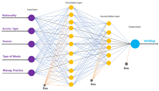
Figure 1.
Optimised ANN structure of 5-11-6-1 selected for forecasting WGR in accommodation sectors.
2.6. Model Performance Evaluation
To evaluate the prediction performance of the models, four statistical indices were applied; the hybrid fractional error function (HYBRID), standard error of prediction (SEP), mean absolute error (MAE) and correlation coefficient (R2) values were derived using the following equations:
where n is the number of observations, wo is the observed values of rate of waste generation for type t, p is the number of independent parameters, wo’ is the average of HSW generation and wp is the predicted value of HSW generation for type t. R2 measures the closeness of the observed data to the predicted data, MAE is a statistical quantity that measures how close predictions are to the eventual outcomes, and SEP is a measure of the accuracy of the predictions. The smaller the value of the error indices for a specified model, the higher the prediction performance of the model [20,21].
3. Results and Discussion
3.1. Results of MLR
The MLR analysis herein was performed using stepwise regression (SPSS 17.0, Chicago, IL, USA). Its p-value was calculated for each input variable and the significant variable was identified following the criteria of having a p-value ≤ 0.05. The MLR was subjected to 3-fold cross-validation procedures, and the averages of the variable estimates were utilised to obtain the regression equation for predicting generation rate of HSW. Multicollinearity was avoided in the final regression equation using a tolerance filter of 0.5:
where A, …, E symbolise the input parameters described in Table 2. The statistical characteristics of the regression equation are represented in Table 3. As obtained, the MLR model indicates that both waste management practice (E) and accommodation type (B) are highly significant parameters, followed by season (C), which is slightly significant and influenced the generated waste quantity with an α-level less than 0.1.
Table 3.
Statistical characteristics of the developed MLR model.
3.2. Analysis of AAN Model Results
In the current study, 138 experimental datasets were fed into the ANN network and randomly classified. Of these, 68% of the datasets were trained, 18% were tested and the remaining 14% were validated. The three-layered feedforward neural network herein consists of the logsig transfer function at hidden layer and a linear transfer function (purelin) at the output layer. To minimise network error, numerical overflows and achieve higher homogeneous results, the model inputs and output were normalised and scaled in the rank of 0.1 to 0.9 using Equation (9):
where the normalised value of the output variable is X*, and X, Xmax and Xmin represent their actual, maximum and minimum values, respectively.
The connection weights of the trained ANN with the corresponding bias terms were employed to estimate the relative significance of each independent variable (Ii) on waste generation rate (kg/day) as given in Equation (10):
where Ii is the relative importance of the ith input variable on the response; W, Ni and Nh represent the connection weights, numbers of input and hidden neurons, respectively. The subscripts ‘k’, ‘m’ and ‘n’ is the input, hidden and output neuron, while the superscripts ‘i’, ‘h’ and ‘o’ represent the input, hidden and output layers, respectively.
3.2.1. Selection of Backpropagation (BP) Training Algorithm
Ten BP algorithms were investigated to select the best BP training algorithm, as depicted in Table 4. The highest value of the degree of correlation (R2) and the least mean square error (MSE) were used as the yardstick to select the best BP. Of all the BP algorithms examined, the Levenberg–Marquardt (LMA) BP algorithm specifically resulted in the least mean square error (0.0014) and its R2 value (0.989) is closest to unity. Hence, LMA was selected as the training algorithm in this research.
Table 4.
Comparison of backpropagation algorithms.
3.1.2. Optimisation of Neuron Number
To obtain an optimised ANN structure, robust networks were constructed by varying the iteration, hidden neurons and learning rates. Our networks were trained perfectly with over 1000 iterations and the optimal learning rate was 0.2, as listed in Table 5.
Table 5.
The parameters of the optimised ANN model used in this study.
The assessment of MSE during training and testing for an optimum number of neurons in the hidden layers is presented in Table 6. As seen in the training set, the MSE was 0.0923 when 13 neurons were used and decreased to 0.0131 when 17 neurons were utilised. The MSE reached a minimum level and increasing the number of neurons beyond 17 does not decrease the MSE further. Hence, 17 neurons were chosen as optimum for the developed ANN topology shown in Figure 1.
Table 6.
Optimisation of neuron number at hidden layer, using testing and training data set.
The optimised neural network model was used to predict the amount of waste generated in two different seasons (peak and lean) by considering a different type of waste. The comparison between the ANN predictive values, CCD, MLR and the actual values is shown in Figure 2.

Figure 2.
Type and amount of waste generated per day in each season (a–c), and actual and predicted average daily waste generated per (d) small hotel, (e) medium hotel, and (f) large hotel.
As shown in Figure 2a–c, food waste is the most generated waste in all the investigated facilities. In the lean season, a total of 970 kg of food waste was generated per day, while this figure increased by almost 1.9% in the peak season. Organic waste (vegetables, milk, bread, etc.) is also commonly generated in all facilities. A total of 415 kg/day of organic waste is generated during the peak season, when the large hotels account for 57%, small hotels 23.4% and medium hotels 19.6%. During the lean season, the organic waste generated decreased to 178.5 kg/day; small hotels generated the least (19.7%). The least generated waste in all the facilities appears to be wood. Only 61 kg/day of wood was generated during the peak season and 28 kg/day was generated during the lean season.
Figure 2d–f, represents the average waste generated per day. During the peak season, the average waste generated was 106.5, 239.5 and 340.9 kg/day by small, medium and large hotels, respectively. Meanwhile, the average waste generated decreased to about 63% during the lean season. As mentioned, the type of waste management practices in each facility has a significant influence on the waste generation rate, as does the nationality of the tourists visiting the facilities.
The nationality influences the environmental performance in each facility [26]. For instance, based on our research, hotels that have tourists from Arab countries have high food wastage, while those with guests from Britain presented high water consumption and more organic waste, which could be attributed to lifestyle. Regarding the nationality of most tourists visiting the investigated facilities, about 33% British visited the facilities followed by Russian (18%), Turkish (16%), Scandinavian (10%), German (8%), Arab (7%), French (5%) and African (3%).
Figure 3a–c shows the observed waste generation rate (%) per day based on the tourist nationality considering peak season. In a small hotel, 19.21% waste is generated by British tourists per day (85.6 kg), Turkish tourists generated 65.8 kg waste, which is 16.29 WGR (%)/day, and the least waste was generated by French tourists (5.67%) per day. A similar pattern is observed in medium-sized hotels; however, Arabs generated the least waste, accounting for 2.2% WGR per day. In contrast, Turkish tourists generated the most waste in large hotels (19.16%), followed by the British (15.1%), and the least waste was generated by Asians (6.9%) in large hotels. This research has helped us to understand the pattern of visitors in each facility and their range of waste generating practices.

Figure 3.
Waste generation rate (%)/day based on tourist nationality (a–c) and based on the type of waste management practice in each facility (d–f) during the peak season.
The waste generation rate per type of facility based on the type of waste management practices is shown in Figure 3d–f. Many hotel facilities take very little action to reduce their environmental impact; specifically, small hotels regard their environmental responsibility as a secondary objective [27]. In most cases, small hotels commonly generate low quantities of waste that are unattractive to waste recycling firms since they often require specific quantities of waste to be collected [27,28]. In this research, the WGR/day of small hotel firms without any waste management practices is 30%, while the WGR of those that engaged in landfill practice is 40% per day. In medium-sized and large hotels without waste management practices, 50% and 70% of WGR, respectively, was observed per day. This is largely due to their increased room occupancy and higher range of waste generating services compared with small hotels.
The ANN prediction appears to be in reasonable agreement with the observed data. More deviation between the actual (residuals) and predicted values was observed in the CCD and MLR models than in the ANN model. Hence, the higher predictive capacity of the ANN can be attributed to its universal capability to approximate complex nonlinear systems, whereas CCD is effective if the system is restricted to second-order polynomial regression [22,29].
3.3. Analysis of CCD
The correlation between the response (WGR) and independent factors (Table 2) was developed using the CCD of the SigmaXL software (ver. 7.0, Ontario, Canada). The standard deviation and correlation coefficient were utilised to evaluate the fitness of the models developed. The smaller the standard deviation and the closer the R2 value to unity, the better the model is at forecasting the response [19]. Table 7 indicates that the quadratic model was not aliased and has a comparatively low standard deviation of 3.361 and relatively high R2 value of 0.9985, which is in reasonable agreement with the predicted R2 (0.9966). Also, the PRESS of the quadratic equation is low (169.23), which revealed the reliability and better precision of the experimental results. Hence, the results indicate that the quadratic model can be used to describe the relationship between the response (WGR) and the interacting variables. Hence, the codified quadratic equation after eliminating the insignificant terms is shown in Equation (11):
Table 7.
Model Summary statistics and ANOVA for the regression model for WGR.
The obtained quadratic equation was further evaluated using ANOVA. As tabulated, the quadratic model for HSW generation rate has an F-value of 329.55 and a p-value of 0.0012, implying that the model is significant. For the model terms, the largest F-value signifies the most significant effect on the response variable and the model term with a p-value less than 0.05 is significant [30]. In this case, the significant model terms are A, B, C, E, AB, BE, A2, B2 and E2, while C2, BC and AE are insignificant. The model term having the most significant effect on the response is B with an F-value of 679.87. The “Lack of Fit” F-value of 1.76 signifies that it is not significant relative to the pure error and there is a 65.88% chance that its F-value being this large could be due to noise [22]. The non-significant “Lack of fit” for WGR indicated the good predictability of the model.
The variability of the independent variables was evaluated based on the results of Equation (11); the negative value of the coefficient A (−8.78) indicates that as the nationality of the tourists changes from 1 to 9, as coded in Table 1, the HSW generation rate decreased. We inferred that British tourists generate more waste than Arab tourists. The positive values of the coefficients indicate that these parameters had a positive effect on the HSW generation rate. For instance, the smaller hotels generate less waste compared to the large hotels with a range of services and greater room occupancy. The interactive influence of the independent variables was investigated and depicted via three-dimensional (3D) response surface plots. The 3D surface plots are very effective at observing complex systems in which two or more variables are significant [31,32,33].
As shown in Figure 4a, the interaction between the season (C) and the type of waste management practice (E) in each facility indicates increased HSW generation rates as C tended towards the peak season (2.5) with accommodation sectors without waste management practices. Figure 4b indicates that the HSW generation rate increased from 65% to 85% in a facility without proper waste management practices, specifically with tourists in the range 1−4 (Table 1). Figure 4c shows that about 44% WGR was observed in the lean season for tourists of nationality 7−9; however, the WGR increased beyond 80% in the lean season when tourists of nationality 1−5 occupied these facilities. Figure 4d depicts the interactive influence of accommodation type (B) and tourists’ nationality (A). According to Equation (10), AB is statistically significant (p = 0.0002 < 0.05) and the WGR increased as the accommodation type changed from small to large hotels as the tourist nationality increased from 1 to 9. This indicates that the WGR is higher at large hotels irrespective of the nationality of the tourists.

Figure 4.
Response surface plots for interactive influence of independent parameters on the WGR. Waste generation rate (%) as a function of (a) season and management practice (b) management practice and tourist nationality (c) season and nationality (d) accommodation type and nationality
3.4. Estimation of Waste Generated and Comparison of Predictive Performance of Models
Forecasting of HSW generation can be classified into short-term (ranging from days to few months), mid-term (few months to 2–4 years) and long-term forecasting (> 5 years). Table 8 summarises the estimated total waste generated by each facility investigated and comparative predictive performance of each model. Herein, statistical analysis was performed to compare the constructed ANN, CCD and MLR models, in terms of their predictive performance, using HYBRID, R2, MAE and SEP (Equations (4)–(7); Table 8).
Table 8.
Estimated total waste generated and comparison of predictive performance of models
The ANN model shows the lowest error values and highest R2 compared to the CCD and MLR models. Based on the obtained results, the ANN architecture is more reliable and accurate in terms of predictive capability and fitting to the non-linear relationship between the variables and HSW generation rate. On the other hand, one of the most significant advantages of the CCD-based model is its ability to clarify the interactive effect of the variables on the response (WGR), which highlights its usefulness in predicting the rate of HSW generation. Hence, combining the abilities of CCD and ANN models in a hybrid fashion could result in powerful modelling and predictive models.
3.5. Sensitivity Analysis and Relative Importance of Input Variables
Figure 5 shows the relative significance of the independent variables on the response (WGR) obtained from Equation (10). It is important to stress that all the input variables had an impact on the waste generation rates. However, the accommodation type (B) seemed to be the most influential variable on WGR, while the second most influential variable was the season (C), followed by waste management practice (E), nationality (A) and type of waste (D), according to ANN. Meanwhile, the CCD and MLR tend to deviate slightly from the ANN predicted data, as shown in Figure 5. The desirability function (D) was applied to select the acceptable ranking and the minimum, middle and maximum values of desirability were configured as D = 0.0, 0.5 and 1.0, respectively. A desirability value closer to 1.0 means that the corresponding sensitivity analysis is able to represent the actual scenario. Hence, the ranking based on the models is as follows; ANN (D = 0.99) > CCD (D = 0.78) > MLR (0.65). It is inferred that the ANN can be employed to simulate and predict the complex independent variable behaviour in any form of non-linearity and can effectively overcome the limitation of quadratic correlation assumed in CCD and MLR.
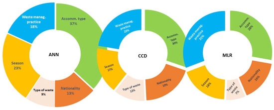
Figure 5.
Relative importance of input variables on WGR forecasted by ANN, CDD and MLR.
4. Conclusions
The accommodation sector is an essential component of the tourism and travel business. It is worth mentioning that increases in hospitality sector operations result in increased quantities of municipal waste, constituting ecosystem damage and a significant increase in the environmental footprint. To curtail the ugly face of tourism activities, precise prediction of the quantity of hospitality waste generated is required to enable the development of an integrated waste management and reutilization system. Note that inaccurate prediction of hospitality waste generated may result in a negative impact on the environment.
For the first time, this study has shown that municipal waste from hospitality facilities can be forecasted by considering measurable and effective parameters via an artificial neural network-inspired forecasting model. The hospitality waste generation rates were analysed based on three categories: recyclable, general waste and food residue. ANN, CCD and MLR were employed to predict the average HSW generation rate using nationality, type of waste, season, accommodation type, and type of waste management practices as predictors. These predictors were selected based on the correlation test and Cronbach’s alpha of 0.93. The results showed that 4159.9 kg (recyclable: 58.5%, general waste: 23.6% and food residue: 17.9%) and 2063.4 kg (recyclable: 33.6%, general waste: 18.5% and food residue: 47.9%) of waste were generated during the peak and lean season from the 22 hospitality facilities investigated, respectively.
Importantly, the use of the ANN model to predict the average HSW generation rate led to reliable results and the difference between the observed and predicted values was not statistically significant. However, the MLR model demonstrated lower prediction accuracy compared to CCD. It was found that Turkish tourists generated more waste (19.16% WGR/day) in large hotels compared with the British (15.1% WGR/day), and Asians generated the least average waste (20.96%) in all the facilities investigated. The findings of this study imply the need for further research to investigate the possible sources of the waste and factors limiting hotels from managing the waste effectively. In conclusion, the results herein are promising and would be useful in establishing a sustainable waste management plans.
Author Contributions
S.L.A. conducted the research and prepared the initial draft; A.A.O. designed the research methodology, analysed the data and co-supervised the research; R.V. applied the statistical analysis; H.A. supervised the project; all of the authors contributed to the data analysis.
Acknowledgments
The authors would like to thank the editor and reviewers for their valuable comments to improve the quality of the paper. More specifically, Soolmaz L. Azarmi wish to acknowledge the valuable contributions of Akeem Oladipo regarding the improvement of the quality, coherence, and content of the paper.
Conflicts of Interest
The authors declare no conflict of interest.
References
- Çiçek, D.; Zencir, E.; Kozak, N. Women in Turkish tourism. Waste Manag. 2017, 31, 228–234. [Google Scholar] [CrossRef]
- Mateu-Sbert, J.; Ricci-Cabello, I.; Villalonga-Olives, E.; Cabeza-Irigoyen, E. The impact of tourism on municipal solid waste generation: The case of Menorca Island (Spain). Waste Manag. 2013, 33, 2589–2593. [Google Scholar] [CrossRef] [PubMed]
- Shamshiry, E.; Nadi, B.; Mokhtar, M.B.; Komoo, I.; Hashim, H.S.; Yahaya, N. Integrated Models for Solid Waste Management in Tourism Regions: Langkawi Island, Malaysia. J. Environ. Public Health 2011, 2011, 709549. [Google Scholar] [CrossRef] [PubMed]
- Arbulú, I.; Lozano, J.; Rey-Maquieira, J. Tourism and solid waste generation in Europe: A panel data assessment of the Environmental Kuznets Curve. Waste Manag. 2015, 46, 628–636. [Google Scholar] [CrossRef] [PubMed]
- Hanifzadeh, M.; Nabati, Z.; Longka, P.; Malakul, P.; Apul, D.; Kim, D.S. Life cycle assessment of superheated steam drying technology as a novel cow manure management method. J. Environ. Manag. 2017, 199, 83–90. [Google Scholar] [CrossRef] [PubMed]
- Molino, A.; Larocca, V.; Chianese, S.; Musmarra, D. Biofuels Production by Biomass Gasification: A Review. Energies 2018, 11, 811. [Google Scholar] [CrossRef]
- Oladipo, A.A.; Ifebajo, A.O. Highly efficient magnetic chicken bone biochar for removal of tetracycline and fluorescent dye from wastewater: Two-stage adsorber analysis. J. Environ. Manag. 2018, 209, 9–16. [Google Scholar] [CrossRef] [PubMed]
- Kim, D.S.; Hanifzadeh, M.; Kumar, A. Trend of biodiesel feedstock and its impact on biodiesel emission characteristics. Environ. Prog. Sustain. Energy 2018, 37, 7. [Google Scholar] [CrossRef]
- Oladipo, A.A.; Ifebajo, A.O.; Nisar, N. High-performance magnetic chicken bone-based biochar for efficient removal of rhodamine-B dye and tetracycline: Competitive sorption analysis. Water Sci. Technol. 2017, 76, 373–385. [Google Scholar] [CrossRef] [PubMed]
- Beigl, P.; Lebersorger, S.; Salhofer, S. Modelling municipal solid waste generation: A review. Waste Manag. 2008, 28, 200–214. [Google Scholar] [CrossRef] [PubMed]
- Batinic, B.; Vukmirovic, S.; Stanisavljevic, N.; Ubavin, D.; Vukmirovic, G. Using ANN model to determine future waste management targets-case study of Serbia. J. Sci. Ind. Res. 2011, 70, 513–518. [Google Scholar]
- Intharathirat, R.; Salam, P.A.; Kumar, S.; Untong, A. Forecasting of municipal solid waste quantity in a developing country using multivariate grey models. Waste Manag. 2015, 39, 3–14. [Google Scholar] [CrossRef] [PubMed]
- Abbasi, M.; Hanandeh, A.E. Forecasting municipal solid waste generation using artificial intelligence modelling approaches. Waste Manag. 2016, 56, 13–22. [Google Scholar] [CrossRef] [PubMed]
- Sha’Ato, R.; Aboho, S.Y.; Oketunde, F.O.; Eneji, I.S.; Unazi, G.; Agwa, S. Survey of solid waste generation and composition in a rapidly growing urban area in Central Nigeria. Waste Manag. 2007, 27, 352–358. [Google Scholar] [CrossRef] [PubMed]
- Xu, L.; Gao, P.; Cui, S.; Liu, C. A hybrid procedure for MSW generation forecasting at multiple time scales in Xiamen City, China. Waste Manag. 2013, 33, 1324–1331. [Google Scholar] [CrossRef] [PubMed]
- Denafas, G.; Ruzgas, T.; Martuzevicius, D.; Shmarin, S.; Hoffmann, M.; Mykhaylenko, V.; Ogorodnik, S.; Romanov, M.; Neguliaeva, E.; Chusov, A.; et al. Seasonal variation of municipal solid waste generation and composition in four East European cities. Resour. Conserv. Recycl. 2014, 89, 22–30. [Google Scholar] [CrossRef]
- Noori, R.; Karbassi, A.; Sabahi, M.S. Evaluation of PCA and Gamma test techniques on ANN operation for weekly solid waste prediction. J. Environ. Manag. 2010, 91, 767–771. [Google Scholar] [CrossRef] [PubMed]
- Constantino, H.A.; Fernandes, P.O.; Teixeirac, J.P. Tourism demand modelling and forecasting with artificial neural network models: The Mozambique case study. Tékhne-Rev. Appl. Manag. Stud. 2016, 14, 113–124. [Google Scholar] [CrossRef]
- Oladipo, A.A.; Gazi, M. Nickel removal from aqueous solutions by alginate-based composite beads: Central composite design and artificial neural network modeling. J. Water Process. Eng. 2015, 8, e81–e91. [Google Scholar] [CrossRef]
- Jahandideh, S.; Jahandideh, S.; Asadabadi, E.B.; Askarian, M.; Movahedi, M.M.; Hosseini, S.; Jahandideh, M. The use of artificial neural networks and multiple linear regression to predict rate of medical waste generation. Waste Manag. 2009, 29, 2874–2879. [Google Scholar] [CrossRef] [PubMed]
- Palmer, A.; Montano, J.J.; Sesé, A. Designing an artificial neural network for forecasting tourism time series. Tour. Manag. 2006, 27, 781–790. [Google Scholar] [CrossRef]
- Zhang, G.P.; Qi, M. Neural networks forecasting for seasonal and trend time series. Eur. J. Oper. Res. 2005, 160, 501–514. [Google Scholar]
- Zhang, G.; Patuwo, B.E.; Hu, M.Y. Forecasting with artificial neural networks: The state of the art. Int. J. Forecast. 1998, 14, 35–62. [Google Scholar] [CrossRef]
- Zorpas, A.A.; Lasaridi, K.; Voukkali, I.; Loizia, P.; Inglezakis, V.J. Solid waste from the hospitality industry in Cyprus. W.I.T. Trans. Ecol. Environ. 2012, 166, 41–49. [Google Scholar]
- Radwan, H.R.; Jones, E.; Minoli, D. Managing solid waste in small hotels. J. Sustain. Tour. 2010, 18, 175–190. [Google Scholar] [CrossRef]
- Maclaren, V.W.; Yu, C.C. Solid waste recycling behavior of industrial-commercial-institutional establishments. Growth Chang. 1997, 28, 93–110. [Google Scholar] [CrossRef]
- Azadi, S.; Karimi-Jashni, A. Verifying the performance of artificial neural network and multiple linear regression in predicting the mean seasonal municipal solid waste generation rate: A case study of Fars province, Iran. Waste Manag. 2016, 48, 14–23. [Google Scholar] [CrossRef] [PubMed]
- Dutta, M.; Ghosh, P.; Basu, J.K. Application of artificial neural network for the decolorization of direct blue 86 by using microwave assisted activated carbon. J. Taiwan Inst. Chem. Eng. 2012, 43, 879–888. [Google Scholar] [CrossRef]
- Azarmi, S.L.; Alipour, H.; Oladipo, A.A. Using artificial neural network and desirability function to predict waste generation rates in small and large hotels during peak and lean seasons. In Proceedings of the 7th Advances in Hospitality & Tourism Marketing & Management (AHTMM 2017) Conference, Famagusta, Cyprus, 10–15 July 2017; pp. 539–547. [Google Scholar]
- Oladipo, A.S.; Ajayi, O.A.; Oladipo, A.A.; Azarmi, S.L.; Nurudeen, Y.; Atta, A.Y.; Ogunyemi, S.S. Magnetic recyclable eggshell-based mesoporous catalyst for biodiesel production from crude neem oil: Process optimization by central composite design and artificial neural network. C. R. Chim. 2018, 21, 684–695. [Google Scholar] [CrossRef]
- Aslani, M.A.A.; Celik, F.; Yusan, S.; Aslani, C.K. Assessment of the adsorption of thorium onto styrene–divinylbenzene-based resin: Optimization using central composite design and thermodynamic parameters. Process. Saf. Environ. Prot. J. 2017, 109, 192–202. [Google Scholar] [CrossRef]
- Teixeira, J.P.; Fernandes, P.O. Tourism time series forecast with artificial neural networks. Tékhne-Rev. Appl. Manag. Stud. 2014, 12, 26–36. [Google Scholar] [CrossRef]
- Oladipo, A.A.; Gazi, M. Targeted boron removal from highly-saline and boron-spiked seawater using magnetic nanobeads: Chemometric optimisation and modelling studies. Chem. Eng. Res. Des. 2017, 121, 329–338. [Google Scholar] [CrossRef]
© 2018 by the authors. Licensee MDPI, Basel, Switzerland. This article is an open access article distributed under the terms and conditions of the Creative Commons Attribution (CC BY) license (http://creativecommons.org/licenses/by/4.0/).