Analysis of Energy Sustainability in Ore Slurry Pumping Transport Systems


1
Escuela de Ingeniería Mecánica, Pontificia Universidad Católica de Valparaíso, Valparaíso 2340025, Chile
2
Thermal Sciences and Fluids Department, Federal University of São João del-Rei, São João del-Rei-Minas Gerais 36307-352, Brazil
*
Author to whom correspondence should be addressed.
Sustainability 2019, 11(11), 3191; https://doi.org/10.3390/su11113191
Submission received: 6 May 2019
/
Revised: 27 May 2019
/
Accepted: 4 June 2019
/
Published: 7 June 2019
(This article belongs to the Section Energy Sustainability)
Abstract
:The mining industry is characterized by a high consumption of energy due to the wide diversity of processes involved, specifically the transportation of ore slurry via pipeline systems. This study investigates the relationship among the variables that define the slurry transportation system to minimize the power requirements and increase energy sustainability. The energy indicator (I), the criterion used for the energy assessment of three different pumping system layouts, was computed via numerical simulation. Optimization of response I was carried out through a statistical technique in the design of the experiment. In the study, four variables were defined to describe the slurry transportation systems, two of which are associated with the piping system (length L and diameter D); the other two are related to the slurry pattern (the volumetric concentration Cv and granulometry D50). The results show that all variables are statistically significant relative to the indicator I, with L having the greatest amplitude of variation in the response, increasing the energy indicator by approximately 60%. Likewise, the decrease of the D50 from 300 µm to 100 µm produces an average decrease of I of 24%. Moreover, the interaction among the factors indicates that two pairs of factors are correlated, namely D50 with L and D with L. Finally, a predictive model obtained a fit that satisfactorily relates with the numerical data, allowing, in a preliminary way, to identify the minimum power requirement in iron ore slurry pipeline systems.
1. Introduction
The Brazilian economy is strongly influenced by the behavior of the mining sector. According to the Brazilian Mining Institute [1,2], the contribution of the mineral production reached upwards of 4.8% of the Brazilian gross domestic product (GDP) in 2018. The GDP from mining in Brazil increased to Brazilian real-BRL 2717.82 million in the fourth quarter of 2018. Mining production in Brazil averaged 2.82% from 2003 until 2019, reaching an all-time high of 21.4% in January of 2010. The World Trade Statistical Review 2018 ranks Brazil eighth in the world’s iron ore exportation, and third in the last year, behind only India and the Russian Federation.
As result of all mining activities, large quantities of products are generated from beneficiation processes, part of which is destined for trading or later processing, while another part is designated for storage in a tailing dam. For transport, the iron ore is mixed with water to form slurry. Currently, there is a consensus that among the many different types of transportation systems, pipeline transport is the most efficient, mainly for systems with high throughputs [3,4,5,6,7].
The design and operation of these slurry transportation systems and, in particular, the performance of the utilized pumps, strongly depend on the properties of the slurry. These properties are a function of the quantity (concentration), size distribution (granulometry), and shape of the ore particles mixed in the water. Unlike the transport of fluids with low viscosity (e.g., water), slurry transportation is much more complex and demands greater power consumption due to the requirement that the fluid velocity be kept greater than the particle deposition velocity.
As a consequence, a hydraulic transport system must be designed and executed carefully so as to achieve the minimum pumping transport cost for specific slurry characteristics. The system costs are related to efficiency in the energy conversion, wherein “efficiency” has several possible interpretations [8]. These interpretations can be related, for example, to the availability of natural resources, to a better understanding of the processes, or to any other novel approach proposed by considering the importance of using relevant efficiency concepts in calculating the energy cost of pumping liquids.
In this sense, significant research efforts have been given towards establishing the appropriate features to ensure the efficient transport of slurries. The authors of [9], motivated by a particularly constraining absence of water in Chile, analyzed energy efficiency in long-distance slurry transport by considering the cost of water in addition to energy cost. According to this criterion, when water is considered in the costs of a transportation system, the optimal concentration of the solids to be transported is an increasing function of the throughput. This result improves early findings, in which the weight of transported material relative to the use of water was not correctly defined [10,11].
An energy indicator I, which is based on thermodynamic principles, has been recently used for the assessment of ore slurry transportation systems based on positive displacement pumps [12] and centrifugal pumps [13] to characterize minimum power consumption based on the above four defined variables. Two of these variables represent the solid to be transport and are used to define the physical properties of the slurry (the volumetric concentration Cv and granulometry D50), while the other two are used for the topological characterization of the pumping system (the pipeline length L and diameter D). In the aforementioned studies, the energy indicator was defined as the energy needed to move 1 m3 of slurry according to specific operating conditions.
The most applicable relationship between these variables could be obtained using the design of experiments (DOE) (see [14]). When simulations are considered as experiments as in the present study, it is possible to apply the same strategies existing for experiments to the simulations [15]. The DOE has been used successfully to analyze and optimize different processes through experimental [16] or computational studies [17,18]. This technique of organization and performance the experiments have an advantage over the traditional ones, requires fewer experiments to obtain the same precision in the estimation of the meta-model [19].
Mining industries are typically located in regions with rugged topography. Consequently, the design of slurry conveyance systems should consider this fact and should be constructed with considerable care and should take into account the different situations in accordance with financial, geographical, and logistical conditions. In this regard, the present study aims to determine the best combination of the four independent variables characterizing the application of relatively short-distance slurry pumping systems to minimize the energy requirement. The methodology developed in [12,13] will be applied in three different slurry transportation systems. All variables are significant relative to I with a similar trend for the three pumping systems. That is, the power requirement is lower when L, D50, and Cv are at their lower levels, and when D is at its higher level. Regarding second-order interactions, the most significant effect can be observed between L and D. Moreover, the surface response model obtained for the three layouts fit the numerical data satisfactorily, with differences of less than 10%. Finally, the optimization of I showed that the minimum value was obtained for Cv = 5%, D50 = 100 µm, L = 500 m and D varying between 227 mm and 235 mm as a function of the pumping system.
2. Materials and Methods
2.1. Description of the Slurry Transportation Systems
Figure 1 illustrates a schematic representation of the different pumping systems used in this study. In general, the systems consist of two reservoirs, a piping system and the pumps. According to the objectives of this research, the main difference between the pumping systems is associated with the number of pumps and their location within the systems. In the first case (the 1P configuration), only one pump is employed, and it is located 5 m from the suction tank (tank placed to the left in Figure 1). In the second system (the PS configuration), two pumps are connected in series and are installed inside a pumping station, also at 5 m from the suction tank. The third layout (the uniformly-distributed, or UD, configuration) utilizes two pumps that are located in different places along the conveyor system. The first one is located at 5 m from the suction tank, while the second one is placed exactly at the midpoint of the system (i.e., half of the pipeline length and at the midpoint of the geometric elevation).
In the suction tank, the solid particles of iron ore are mixed with the carrier fluid (water) to form the slurry that is designated for storage at the tailing dam (the reservoir on the right side of Figure 1). Both reservoirs are represented as large tanks, i.e., the velocity of the free surface may be considered as zero, and the pressure on this surface is atmospheric.
2.2. Characteristics of the Piping Systems
To define the layout of the different studied system’s, two considerations were carefully evaluated. The first one is that the defined layout corresponds to the typical topological characteristics where mining industries are located in the region under study, i.e., the state of Minas Gerais/Brazil, which are characterized by topological elevation up to 40 m between the industry and the iron ore storage dam. The second consideration is related with the selected independent factors for the study, both for the iron ore slurry and for the piping system, insomuch that the values were chosen in accordance with typical values of the mining industry.
The piping system has a similar layout for all cases studied, as shown in Figure 1. The pipeline that extends from the suction reservoir to the pumping station, i.e., the suction system, is a straight segment 5 m in length. The discharge system that extends from the pumping station to the tailing dam comprises pipes arranged along horizontal and inclined orientations and the minimum number of fittings required for proper operation of the system.
Two independent variables corresponding to slurry transportation systems were defined: the pipe length L and the diameter D. The values selected for these two variables agreed with the criteria used in the mining industry. The selected values for pipe length range between 500 m (lower value) and 2000 m (higher value). For all cases, the horizontal pipe after the pumping station and the inclined pipe have the same lengths. To keep the system length constant during the simulation, possible adaptations to the length of the final horizontal section length immediately prior to the discharge tank may be applied. The pipe diameter ranges from 200 mm (lower value) to 250 mm (higher value). A topological elevation of 40 m was kept constant for all cases [20].
2.3. Description and Rheology of the Slurry
Slurry Rheology
In this study, the pumped media is a settling slurry. The slurry is formed by solid particles of iron ore mixed with water as carrier fluid. The main physical properties of iron ore slurry were determined by applying the typical equations from the classical literature. As the study here presented is focused on slurry with small concentration of solid (Cv up to 10%), the rheological model used [21] treat the slurry and the carrier fluid with constant properties.
The slurry dynamic viscosity μs (Pa.s) is computed by Equation (1), [22],
where μl is the dynamic viscosity of carrier fluid (water) and Cv (decimal) is the volumetric concentration of solid in the slurry.
The slurry density ρs (kg/m3), can be determined by Equation (2), [21,22],
where ρp is the density of the dry solid (iron ore), ρl is the density of the carrier fluid (water), and Cw is the concentration of solids by weight in the slurry (%). For iron ore (dry), the density is 3110 kg/m3. For water, the temperature assumed to be 24 °C; therefore, physical properties are ρ = 997.42 kg/m3 and μ = 0.000908 Pa.s.
The relation between the concentration of solids Cw (%) and the volumetric concentration Cv (%), is given by Equation (3),
Ss and Sp are the specific gravity of the slurry and dry solid, respectively.
The influence of the granulometry on the slurry transportation it is considered by the semi-empirical Wilson–Georgia Iron Works model (Wilson-GIW) [21], which computes the energy dissipation due to the presence of solid particle in a carrier flow as expressed by Equation (4),
where Im is the hydraulic gradient for slurry flow [-], If is the hydraulic gradient for carrier flow [-], Cv is the volumetric concentration of solid in slurry [decimal], Sp is the specific gravity of solid [-], Vs is the mean velocity of the slurry in the pipeline [m/s], V50 is the value of Vs when one half of solid is suspended in a carrier flow [m/s] and M is an empirical coefficient [-].
In Equation (4), both V50 (Equation (5)) and M (Equation (6)) depend on D50.
D85 is the 85% passing size of solid (μm) and according to Wilson-GIW model, the value of M should not exceed 1.7 nor fall below 0.25.
In the present research, Cv and D50 were considered to range between 5% and 10% and 100 µm to 300 µm, respectively.
2.4. Pumps
The pumps used in this study are centrifugal pumps. To perform an independent analysis of any commercial manufacturer of slurry pumps, and after a wide and careful review of the technical literature [23,24,25], it was decided to designate the pumps used in this study as Pump 1 and to rank them by their operating range, according performance curves, as shown in Figure 2.
As mentioned above, in the PS configuration, the pumps are connected in series. In this case, the resulting head curve for this kind of association is determined by the vertical sum of the head curve shown in Figure 2, that is, for a given flow rate the corresponding head is summed.
In simulations with water, it was assumed the criterion that operational efficiency of the pumps satisfies the following condition: operational efficiency is ≥0.9 of the best efficiency point (BEP) of the pumps. As the efficiency of the pumps when handling slurry is slightly lower to the efficiency handling clear water, this criterion ensures high efficiency for slurry transporting.
3. Methodology
3.1. Numerical Simulations
The AFT Fathom software produced by Applied Flow Technology Inc. was used to perform the numerical simulations. It is a software package designed for the simulation of fluid flows with different rheological behaviors and the pipe flow configurations. This software tightly integrates equipment characteristics, analysis, and output with the system’s schematic representation. It also improves the quality of systems engineering that can be achieved, leading to less costly, more efficient, and more reliable piping systems. The simulations were performed by using a settling slurry modeling (SSL) module that allows, among other capabilities, the modelling of the effects corresponding to pumping fluids containing settling solids.
Although centrifugal pump manufacturers design machines to be specifically used for slurry pumping, their performance curves are defined for clear water because of the inability to previously define specific operating conditions for slurries. Therefore, when a pump is being selected for a slurry application, it is necessary to derate the performance. Hence, the first step in the simulation is to define the operating conditions for each of the systems illustrated in Figure 1 while considering clear water as the pumped fluid. In these cases, the pump performance curves are used, defined as previously established in Figure 2. After these simulations, it is possible to obtain all of the operating parameters: volumetric flow rate, head rise, pump power input, and efficiency.
The head developed by a centrifugal pump that is handling slurry differs from the head of a pump handling water depending upon the amount, size, shape, and specific gravity of solid particles in the slurry. This difference in the head is considered by the head ratio (HR), which is a coefficient defined by the ratio between the head required to transport the slurry over the head necessary for clear water in the same conditions. Similarly, it is also defined by the efficiency ratio (ER), which stands for the ratio between the efficiency required to transport the slurry and the efficiency for clear water in the same conditions. The values of HR and ER can be obtained by means of the Cave’s Abacus [22,26] as function of the factors characterizing the solid in the slurry: the granulometry, the specific gravity S and the dilution of the slurry.
With the operating parameters obtained for clear water and with the values of HR and ER obtained by the use of the Cave’s Abacus, it is possible to determine each of the slurry operating parameters: volumetric flow rate, head rise, pump power input and efficiency, deposition velocity, and head loss of slurry, based on slurry density and on clear water density.
In AFT Fathom, the model selected for the pumps in slurry simulations is head rise-fixed, prescribing the head and efficiency computed by the HR, and head for clear water and the ER and efficiency for clear water, respectively. The energy indicator I, in kWh/m3, expresses the specific energy consumption of the pumps, that is, how much energy is required for pumping 1 m3 of slurry under specific conditions and is defined as follows:
where is the mechanical power of the pumps (W), Q is the volumetric flow rate (m3/s), H is the head (m), ρ is the density of the slurry (kg/m3), and η is the efficiency of the pump (%).
3.2. Design of Experiments
The design of experiments (DOE) is the efficient and applicable statistical methodology to organize the experimentation, allowing the acquisition of the largest amount of information with the fewest number of experiments. In this work, the DOE was used to investigate the relationship between an array of the variables (factors) under control and the measured response.
The first step to apply the DOE methodology is to define the response of interest, the factors, the factors’ levels, and the most adequate kind of design to conduct the simulations. The conditions and the maximum number of the necessary simulations are defined by these data [27].
There are several types of experimental designs; however, the factorial experiments are the most used in the field of research [28]. An experiment is called factorial when in each simulation are simultaneously considered two or more factors with their corresponding levels. The values of each factor in the simulations are known as the factor levels. For constructing the designs, the value of the factor’s levels (natural variables) are usually transformed into dimensionless coded variables where the code −1 is assigned to the lower level and, the code +1 to the higher level of the factor. Commonly, a combination of these signs like the Yates distribution to organize of the simulations is used [29]. The simulations are organized in a simulations’ plan. Every factor has a column in the experimental plan, where the level that the factor will assume in each simulation is fixed.
The full factorial design is, probably, the most common strategy of the DOE. In the simplest form, in the two-level full factorial, there are k factors and two levels per factor. The quantity of the all possible combinations of the factors and their levels are calculated as n = 2k. However, a potential concern when using this type of design is the assumption of linearity of the factor’s effects, which is sometimes compensated by the knowledge of previous studies.
Nevertheless, according to the best knowledge of the authors, no previous research results relate to the application of DOE in the energy assessment or in the design of slurry transportation systems. Therefore, any linearity or trends among the relationships between the factors that define this phenomenon are unknown. For these cases, others designs could be used, for example, the central composite design (CCD).
A CCD is composed by a factorial part, like a full factorial design, plus several axial and center points depending on of amount of factors and the amount of replicas in the experiment. The axial points in this kind of design can be centered in the faces or can be star points. Figure 3 shows the structure of a CCD with axial points centered in the faces, like those used in this study, as an example with two independent variables.
The axial points represent the tests where all factors, except one, are set at their mid-levels and; the center points represent the tests where all factors are set at their mid-levels. For an experiment considering k factors, the total number of simulations n, would be equal to no + 2k + 2k. The number of central points depends heavily on the number of factors and replicas that can be performed.
The response variable (Y) of the CCD could be expressed as the following second-order polynomial equation by using a multiple regression technique:
where Y represents the predicted response, and denote the factors using coded values, is the intercept term which is constant, quantifies of the linear effect of each factor; quantifies the quadratic effect of each factor, and quantifies the interaction effects between two different factors.
Experimental designs and the polynomial coefficients were calculated and analyzed using a windows release standard version of MINITAB (version 17.0). Statistical analysis of the model was performed to evaluate the analysis of variance (ANOVA) considering a confidence interval of 95%. p-values smaller than 0.05 were considered significant.
For this research, the response selected was the energy indicator I. The analyzed factors with regard to the piping system were the length L, the diameter D; and the volumetric concentration Cv and the granulometry D50, relative to the slurry’s properties. The levels, low and high, of these variables were previously defined. Moreover, to apply this CCD technique, a central value for each factor was defined as: L = 1000 m, D = 225 mm, Cv = 7.5%, and D50 = 200 µm. The design selected was a CCD with axial points centered in the faces, that with four factors results in a simulation plan with 31 simulations (16 factorial points, 8 axial points, and 7 center points) recommended by the MINITAB, (see Table 1). In case of the center points, as required to obtain a response surface that can be optimized, the designs of experiments selected add center points in order to estimate the curvature in the adjusted data [28]. These 31 simulations were performed in each of the three system configurations.
4. Results and Discussion
A total of 93 simulations were carried out, and the influence of each the four factor on the energy indicator I was analysed. Later, the values of I obtained in the parametric study were used to fit the response surface models, which include the main effects of the independent variables, the effects of the interactions among them and the quadratic terms.
Figure 4 depicts the main effects that the level changes of L, D, D50, and Cv have on I for each of the slurry piping system configurations. Points in the graphs correspond to the arithmetic mean of I in each level of each factor; the average effect of each factor on the response is evidenced. As shown in Figure 4, the behaviour of the response I, due to the variation of the factors from one level to another, has the same trend regardless of the slurry piping system. Among the four variables, L has the greatest amplitude of variation between the highest and the lowest level. The minimum values of I are reached when L, Cv, and D50 are at their lower levels and when D is at a higher level.
These results can be best explained from a fluid mechanics point of view. The increase of L, from 500 m to 2000 m, keeping other factors equal, promotes a significant increase of approximately 60% of the indicator I in all cases investigated. By applying an energy balance it is possible to demonstrate that, when the system length increases, there is an increase in distributed head losses and, consequently, the pump must thus provide a higher energy (per unit weight) to transport the slurry to the tailings dam. The factor L has the greatest effect on the energy consumption for all of the analysed systems.
The change in pipe diameter from 200 mm to 250 mm promotes an average reduction of 22.4% of I in all simulations conducted, keeping all other factors constant. It is well-known when the pipe diameter increases, the hydraulic losses, defined by the sum of the distributed head losses and the minor head losses, decreases and, consequently, the required power by the system is lower.
A change from the lower level to the higher level of granulometry, that is, from 100 μm to 300 μm, produces an average increase of I of 24%, keeping the remaining variables constant. By increasing the granulometry, the size, and, consequently, the weight of the solid grains in the slurry also increase. To avoid the sedimentation of particles, a greater energy should be supplied to increase the slurry flow velocity.
The volumetric concentration has the smallest effect on I when compared with other factors, wherein an average increase of I of 9.2% occurs when Cv varies from its lower (5%) to higher level (10%). The influence of Cv on I can be explained by the increase of the solid volume in the slurry.
Apart from these main effects, the interactions among the factors were also investigated and it was determined that the only significant interactions on I are those between D50 and L, as well as between D and L, for all pumping systems examined.
The interaction between these two pairs of variables is shown in Figure 5. At the top of the figure, it is possible to observe the relationship among D50, L and I for the three system configurations studied. The granulometry exerts almost no influence when L is at its higher level, but its significance rises noticeably as L decreases to its lower levels.
At the bottom of the figure, it is possible to observe the relationship among D, L, and I for the three system configurations. The value of I diminishes as D increases and L decreases. The indicator I has a minimum value when D is approximately 225 mm for a lower value of L. The curvature of the response surface approximately for 225 mm for an L value of 500 m confirms this effect.
The prediction models based on the experiments, which respond by the response surfaces shown above, can be used to predict the response I at any point in the space limited by the levels of the factors in the design, provided that the model has an appropriate fit. The adjustment of the models was studied through normal probability graphs and the calculation of two statistical coefficients used in model adjustment, the coefficient of determination , and the standard error of the regression S.
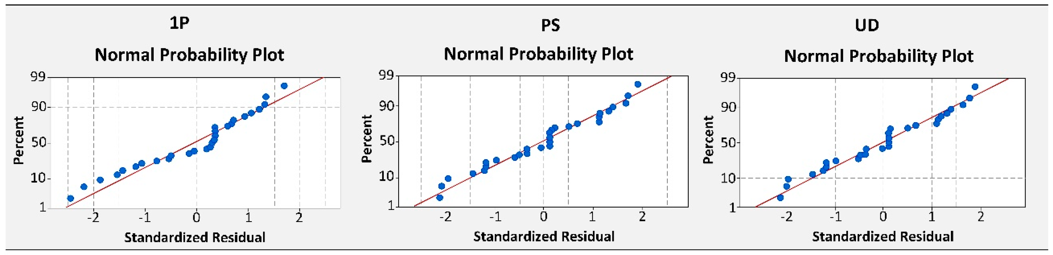
Figure 6 illustrates the normal probability plots of the standardized residuals corresponding to the models for I. From these graphs, the accuracy of each model can be assessed. Firstly, it should be noted that most of the residuals for all cases are low; only two of 31 samples, for each layout, have an absolute value larger than 2, which is the value typically accepted to identify outliers [15]. Secondly, the residuals of three models do not depart substantially from a straight line in the normal probability plot, thus confirming that they are very-nearly normally distributed.
On the other hand, the value of for all experiments is higher than 98%, and the value of S is approximately zero. These values meet the appropriate values for both parameters to accept the models. Hence, the quadratic response surface models employed fit the data satisfactorily.
The predicting models are expressed by Equations (9)–(11), for the 1P, PS, and UD cases, respectively:
For Equation (9), = 0.988 and S = 0.028; for Equation (10), = 0.982 and S = 0.026; and for Equation (11), = 0.981 and S = 0.027.
It is apparent that these models have two components: the linear part, which is associated with the main effects, and the non-linear term, which corresponds to the interactions between the parameters.
Figure 7 illustrates the comparison between the simulation results and the results obtained via the reduced prediction models. As can be observed in the right side of Figure 7, a difference of less than 10% is obtained in all cases, wherein the fitted values are compared with those obtained in the simulations. These results indicate that a good agreement exists between the models and simulations; therefore, an appropriate response for I can be obtained by using the models.
From the obtained models and considering the main objective of the present study, the optimal combination of independent variables required to minimize the indicator I was determined under the assessed conditions and has been showed in Table 2.
The standard interval global engine (SIGE) method, as defined by [30], was applied to obtain the optimal combination. Table 2 shows the optimal combinations of the independent variables for the pumping systems analysed in the range of investigated values. From these results, it is possible to observe that the optimal values for optimizing (minimizing) I are as follows: Cv = 5% (lower level), D50 = 100 μm (lower level), L = 500 m (lower level), and D varying between 227 mm and 235 mm as a function of the pumping system. As is well-known, this value of the diameter is not a normalized value because in the mining industry he commercial pipes has a diameter of 200 mm and 250 mm. Earlier statistical analysis established that 225 mm is the optimal value, but from a practical point-of-view, it is not possible to meet this condition. Therefore, a value of 250 mm was selected. This result is in agreement with the physical foundation of the study phenomena, as previously discussed.
It is important to highlight that the desirability function is an indicator that provides an estimate of the extent to which the solution suggested by SIGE meets the requirements of the response I. The desirability function ranges from 0 to 1, where values close to 1 correspond to a good fit between the results obtained via models and simulations [31,32].
Taking the global results of the optimization into account, it is possible to observe that the indicator I decreases by 11% when the layouts with two pumps (PS and UD) are compared with that of only one pump (1P). It is worth noting that in the 1P configuration, the pump has a higher operating range than the pumps used in layouts PS and UD and thus results in a direct economic impact on operating and maintenance costs. However, the results obtained are unable to explicitly demonstrate whether the PS or UD configuration meets the most effective combination of factors for minimizing I. Choosing the best configuration will likely depend upon other variables not directly associated with the factors studied here. In this case, factors related to logistical conditions in real situations should be analysed.
5. Conclusions
After a careful bibliographical review, and from the results obtained, it is possible to conclude that the slurry transportation system may be characterized by means of four independent variables, two of which are associated with the piping system (length and diameter), while the other two are associated with the physical properties of the slurry (volumetric concentration and granulometry of solid particles). The appropriate relationship amongst them, in order to minimize the power requirement of the conveyor systems, was determined through a numerical study by employing the central composite design technique (combined with the DOE) for optimizing the number of simulations required and analysing the results. The adopted values for the variables correspond to typical values used in the mining industry. To characterize the power requirement, the authors have used an energy indicator I to indicate the energy required to move a unit of slurry within specific operating conditions.
To carry out the analysis, three different slurry transportation systems were assessed. The main difference among them is the quantity of pumps and their location within the systems.
The analysis of the main effects shows that all factors are significant relative to I with a similar trend for the three pumping systems. That is, the power requirement is lower when L, D50, and Cv are at their lower levels and when D is at its higher level. Among the factors, L is the most influential factor when its value changes between its lower and higher levels. From the analysis of the main effects, the minimum values of I are reached when L, Cv, and D50 are at their lower levels and when D is at its higher level. This result has a well-founded theoretical basis and can be explained from a fluid mechanics point-of-view. The interaction among variables, i.e., the second-order interactions, shows that only the relationships between L and D50 and between D and L are significant for I in the three pumping systems investigated. When the effect on I is analysed regarding the interaction between L and D50, it is possible to observe that D50 has different behaviour as a function of the level of L. When L is at its higher levels, the influence of D50 is almost insignificant, but when L trends to lower levels, the significance of D50 is appreciable.
The most significant effect can be observed for factors L and D, resulting in a second-order interaction.
The minimum of I is obtained for D = 235 mm, D = 227 mm, and D = 229 mm for layouts 1P, PS, and UD, respectively. Since no normalized diameter of 225 mm exists, it is suggested to select D = 250 mm for a minimum value of I.
Regression models obtained for the three layouts fit the numerical data satisfactorily, with differences of less than 10%.
An interesting result of this research postulates that between the piping system variables and slurry variables, those related to the piping system are the significant ones.
The results of this work show that through a careful design of the slurry transportation system, numerous benefits can be achieved regarding sustainable development, such as a reduction in water usage and a higher transport of solid throughputs.
Regardless of the reduced interval of values for the variables, the results confirm that the new methodology presented herein, which combines numerical simulation and the design of experiments, has a huge potential to offer relevant information, thereby allowing professionals to establish the appropriate combination of variables to minimize energy consumption in medium-length slurry transportation systems.
Author Contributions
Conceptualization, G.V. and M.T.C., methodology, J.P. and M.T.C.; formal analysis, Y.M. and G.V., investigation, Y.M. and J.P.; software, G.V., validation and statistics, Y.M. and J.P. writing—original draft preparation, J.P.; writing—review and editing, G.V. and Y.M.; project administration, G.V.
Funding
This research received no external funding.
Acknowledgments
The authors are grateful to the Engineering Faculty of the Pontifica Universidad Católica de Valparaíso, Chile, for the financial support through the Proyecto INNOVACHILE 14ENI2-26905 (Ingeniería 2030).
Conflicts of Interest
The authors declare no conflict of interest.
References
- Brazil GDP Growth Rate 2019. Available online: https://tradingeconomics.com/brazil/gdp-growth (accessed on 25 May 2019).
- Fundação Estadual do Meio Ambiente—FEAM. Available online: http://www.feam.br/ (accessed on 25 May 2019).
- Wasp, E.J. Slurry pipelines. Sci. Am. 1983, 249, 48–55. [Google Scholar] [CrossRef]
- Jacobs, B.E. Design of Slurry Transport Systems; Elsevier Applied Science: London, UK, 1991; ISBN 978-1-85166-634-8. [Google Scholar]
- Shirakashi, M.; Yamada, S.; Kawada, Y.; Hirochi, T. Blocking of snow/water slurry flow in pipeline caused by compression-strengthening of snow column. Sustainability 2014, 6, 530–544. [Google Scholar] [CrossRef]
- Ohlan, R.; Gopaliya, M.K.; Kaushal, D.R. Simulation of sand-water slurry flows through pipeline. Multph. Sci. Technol. 2018, 30, 293–318. [Google Scholar] [CrossRef]
- Kumar, N.; Gopaliya, M.K.; Kaushal, D.R. Experimental investigations and CFD modeling for flow of highly concentrated iron ore slurry through horizontal pipeline. Part. Sci. Technol. 2019, 37, 232–250. [Google Scholar] [CrossRef]
- Ihle, C.F.; Tamburrino, A.; Montserrat, S. Computational modeling for efficient long distance ore transport using pipelines. Miner. Eng. 2014, 63, 73–80. [Google Scholar] [CrossRef]
- Ihle, C.F. The least energy and water cost condition for turbulent, homogeneous pipeline slurry transport. Int. J. Miner. Process. 2016, 148, 59–64. [Google Scholar] [CrossRef]
- Wu, J.; Graham, L.; Wang, S.; Parthasarathy, R. Energy efficient slurry holding and transport. Miner. Eng. 2010, 23, 705–712. [Google Scholar] [CrossRef]
- Edelin, D.; Czujko, P.-C.; Castelain, C.; Josset, C.; Fayolle, F. Experimental determination of the energy optimum for the transport of floating particles in pipes. Exp. Therm. Fluid Sci. 2015, 68, 634–643. [Google Scholar] [CrossRef]
- De Barcelos, R.J.P.; de Araujo, E.; Vilalta, G. Influence of the iron ore properties on slurry pumping system with volumetric pumps by applying simulation and Design of experiments. In Proceedings of the Anais Do National Congress of Mechanical and Production Engineering, Novo Hamburgo, Brazil, 24–27 November 2015. [Google Scholar]
- Gava, M. Energy Analysis of Iron Ore Slurry Pumping Systems by Computational Simulation. Master’s Thesis, Federal University of São João del-Rei, São João del-Rei, Brazil, 2016. [Google Scholar]
- Tanco, M.; Viles, E.; Ilzarbe, L.; Alvarez, M.J. Implementation of Design of Experiments projects in industry. Appl. Stoch. Models Bus. Ind. 2009, 25, 478–505. [Google Scholar] [CrossRef]
- Montgomery, D.C. Design and Analysis of Experiments, 9th ed.; Wiley: Hoboken, NJ, USA, 2017; ISBN 978-1-119-11347-8. [Google Scholar]
- Kotcioglu, I.; Cansiz, A.; Khalaji, M.N. Experimental investigation for optimization of design parameters in a rectangular duct with plate-fins heat exchanger by Taguchi method. Appl. Therm. Eng. 2013, 50, 604–613. [Google Scholar] [CrossRef]
- Chiang, K.-T. Modeling and optimization of designing parameters for a parallel-plain fin heat sink with confined impinging jet using the response surface methodology. Appl. Therm. Eng. 2007, 27, 2473–2482. [Google Scholar] [CrossRef]
- Larraona, G.S.; Rivas, A.; Antón, R.; Ramos, J.C.; Pastor, I.; Moshfegh, B. Computational parametric study of an impinging jet in a cross-flow configuration for electronics cooling applications. Appl. Therm. Eng. 2013, 52, 428–438. [Google Scholar] [CrossRef]
- Bursztyn, D.; Steinberg, D.M. Comparison of designs for computer experiments. J. Stat. Plan. Inference 2006, 136, 1103–1119. [Google Scholar] [CrossRef]
- Ferreira, M.T. Energy indicator for analysis of iron ore pumping systems via Numerical Simulation and Design of Experiments. Master’s thesis, Federal University of São João del-Rei, São João del-Rei-Minas Gerais, Brazil, 2016. [Google Scholar]
- Wilson, K.C.; Addie, G.R.; Sellgren, A.; Clif, R. Slurry Transport Using Centrifugal Pumps, 3rd ed.; Springer: New York, NY, USA, 2006; ISBN 978-0-387-23262-1. [Google Scholar]
- Chaves, A.P. Teoria e Prática do Tratamento de Minérios, 1st ed.; Signus: Rio de Janeiro, Brazil, 2009; ISBN 978-85-87803-26-9. [Google Scholar]
- Sheth, K.K.; Morrison, G.L.; Peng, W.W. Slip Factors of Centrifugal Slurry Pumps. J. Fluids Eng. 1987, 109, 313–318. [Google Scholar] [CrossRef]
- Walker, C.I.; Robbie, P. Comparison of some laboratory wear tests and field wear in slurry pumps. Wear 2013, 302, 1026–1034. [Google Scholar] [CrossRef]
- Kumar, S.; Gandhi, B.K.; Mohapatra, S.K. Performance characteristics of centrifugal slurry pump with multi-sized particulate bottom and fly ash mixtures. Part. Sci. Technol. 2014, 32, 466–476. [Google Scholar] [CrossRef]
- Wills, B.A.; Finch, J.A. Wills’ Mineral Processing Technology: An Introduction to the Practical Aspects of Ore Treatment and Mineral Recovery, 8th ed.; Butterworth-Heinemann: Montreal, QC, Canada, 2016; ISBN 978-0-08-097054-7. [Google Scholar]
- Pedrera, J.; Ortiz, J.; Vilalta, J.A. Significant variables in initial dilution process in submarine outfalls systems. Alternatives comparison. In Proceedings of the International Symposium of Outfall System, Ottawa, ON, Canada, 10–13 May 2016; pp. 324–349. [Google Scholar]
- Antony, J. Design of Experiments for Engineers and Scientists; Butterworth-Heinemann: Amsterdam, The Netherlands, 2010; ISBN 978-0-7506-4709-0. [Google Scholar]
- Box, G.E.P.; Hunter, J.S.; Hunter, W.G. Statistics for Investigators: Design, Innovation and Discovery, 2nd ed.; Reverte Editorial Sa: Barcelona, Spain, 2008; ISBN 978-84-291-5044-5. [Google Scholar]
- Hansen, E.R.; Walster, G.W. Global Optimization Using Interval Analysis, 2nd ed.; Monographs and Textbooks in Pure and Applied Mathematics; CRC Press: New York, NY, USA, 2004; ISBN 978-0-8247-4059-7. [Google Scholar]
- Myers, R.H.; Montgomery, D.C.; Anderson-Cook, C.M. Response Surface Methodology: Process and Product Optimization Using Designed Experiments, 3rd ed.; Wiley Series in Probability and Statistics; Wiley: Hoboken, NJ, USA, 2009; ISBN 978-0-470-17446-3. [Google Scholar]
- Murphy, T.E.; Tsui, K.-L.; Allen, J.K. A review of robust design methods for multiple responses. Res. Eng. Des. 2005, 15, 201–215. [Google Scholar] [CrossRef]
Figure 1.
Schematic representation of the simulated piping systems.

Figure 2.
Performance curves for pumps used in this work.

Figure 3.
The scheme of a central composite design (CCD) with two variables and centered in the faces.
Figure 3.
The scheme of a central composite design (CCD) with two variables and centered in the faces.

Figure 4.
Main effects of the parameters on the energy indicator I for each block.

Figure 5.
Main response surfaces in terms of the interacting variables for the Indicator I for the (a) one-pump 1P, (b) two-pump (PS), and (c) two-pump uniformly-distributed (UD) configurations.
Figure 5.
Main response surfaces in terms of the interacting variables for the Indicator I for the (a) one-pump 1P, (b) two-pump (PS), and (c) two-pump uniformly-distributed (UD) configurations.

Figure 6.
Standardized residuals of the response surface for the energy indicator I.

Figure 7.
Comparison among simulations and response surface model for the Indicator I for the (a) one-pump (1P), (b) two-pump (PS), and (c) two-pump uniformly-distributed (UD) configurations.
Figure 7.
Comparison among simulations and response surface model for the Indicator I for the (a) one-pump (1P), (b) two-pump (PS), and (c) two-pump uniformly-distributed (UD) configurations.


Table 1.
Details of the parametric study: values of the parameters considered and their combinations in each simulation (experiment). D: diameter; L: length; Cv: volumetric concentration; D50: granulometry.
Table 1.
Details of the parametric study: values of the parameters considered and their combinations in each simulation (experiment). D: diameter; L: length; Cv: volumetric concentration; D50: granulometry.
| Parameter (Factor) | Values (Levels) | Exp. | Cv | D50 | D | L | Exp. | Cv | D50 | D | L | ||
|---|---|---|---|---|---|---|---|---|---|---|---|---|---|
| Low (−1) | Middle (0) | High (+1) | |||||||||||
| Cv | 5 | 7.5 | 10 | 1 | 0 | 0 | 0 | 0 | 17 | −1 | 1 | 1 | 1 |
| D50 | 100 | 200 | 300 | 2 | 0 | 0 | −1 | 0 | 18 | 0 | 0 | 0 | 0 |
| D | 200 | 225 | 250 | 3 | 1 | 1 | −1 | 1 | 19 | −1 | −1 | 1 | 1 |
| L | 500 | 1250 | 2000 | 4 | 1 | −1 | −1 | 1 | 20 | −1 | −1 | −1 | −1 |
| 5 | 0 | 0 | 0 | 0 | 21 | 1 | 1 | 1 | −1 | ||||
| 6 | −1 | −1 | −1 | 1 | 22 | 1 | −1 | −1 | −1 | ||||
| 7 | 1 | −1 | 1 | −1 | 23 | −1 | 0 | 0 | 0 | ||||
| 8 | −1 | 1 | −1 | 1 | 24 | 0 | 0 | 0 | 0 | ||||
| 9 | 1 | 1 | −1 | −1 | 25 | 0 | 0 | 0 | −1 | ||||
| 10 | 1 | 1 | 1 | 1 | 26 | 0 | 1 | 0 | 0 | ||||
| 11 | −1 | 1 | −1 | −1 | 27 | 1 | 0 | 0 | 0 | ||||
| 12 | 0 | −1 | 0 | 0 | 28 | −1 | 1 | 1 | −1 | ||||
| 13 | 0 | 0 | 1 | 0 | 29 | 0 | 0 | 0 | 0 | ||||
| 14 | 0 | 0 | 0 | 1 | 30 | 1 | −1 | 1 | 1 | ||||
| 15 | 0 | 0 | 0 | 0 | 31 | −1 | −1 | 1 | −1 | ||||
| 16 | 0 | 0 | 0 | 0 | |||||||||
Table 2.
Optimal combination of the independent variables and verification of the results obtained by comparison of the simulation versus the predicted models.
Table 2.
Optimal combination of the independent variables and verification of the results obtained by comparison of the simulation versus the predicted models.
| Case | Cv (%) | D50 (µm) | D (mm) | L (m) | Desirability Function | Energy Indicator | |
|---|---|---|---|---|---|---|---|
| One pump (1P) | Simulation | 5 | 100 | 235 | 500 | 1.00 | 0.261 |
| Model (Equation (9)) | 0.263 | ||||||
| Two pumps (PS) | Simulation | 5 | 100 | 227 | 500 | 0.987 | 0.248 |
| Model (Equation (10)) | 0.233 | ||||||
| Two pumps (UD) | Simulation | 5 | 100 | 229 | 500 | 0.965 | 0.256 |
| Model (Equation (11)) | 0.232 | ||||||
© 2019 by the authors. Licensee MDPI, Basel, Switzerland. This article is an open access article distributed under the terms and conditions of the Creative Commons Attribution (CC BY) license (http://creativecommons.org/licenses/by/4.0/).
Share and Cite
MDPI and ACS Style
Masip Macía, Y.; Pedrera, J.; Castro, M.T.; Vilalta, G. Analysis of Energy Sustainability in Ore Slurry Pumping Transport Systems. Sustainability 2019, 11, 3191. https://doi.org/10.3390/su11113191
AMA Style
Masip Macía Y, Pedrera J, Castro MT, Vilalta G. Analysis of Energy Sustainability in Ore Slurry Pumping Transport Systems. Sustainability. 2019; 11(11):3191. https://doi.org/10.3390/su11113191
Chicago/Turabian StyleMasip Macía, Yunesky, Jacqueline Pedrera, Max Túlio Castro, and Guillermo Vilalta. 2019. "Analysis of Energy Sustainability in Ore Slurry Pumping Transport Systems" Sustainability 11, no. 11: 3191. https://doi.org/10.3390/su11113191
Note that from the first issue of 2016, this journal uses article numbers instead of page numbers. See further details here.