Climate Impacts on Capital Accumulation in the Small Island State of Barbados


1
US Center, Stockholm Environment Institute, Somerville, MA 02144, USA
2
Department of Civil and Environmental Engineering, Tufts University School of Engineering, Science & Engineering Complex, Anderson Hall, Medford, MA 02155, USA
3
Brighton Business School, University of Brighton, Mithras House, Lewes Road, Brighton BN2 4AT, UK
4
BlueGreen Initiative Inc., Peterkin Road, St. Michael, Barbados
*
Author to whom correspondence should be addressed.
Sustainability 2019, 11(11), 3192; https://doi.org/10.3390/su11113192
Submission received: 9 May 2019
/
Revised: 31 May 2019
/
Accepted: 4 June 2019
/
Published: 7 June 2019
(This article belongs to the Section Economic and Business Aspects of Sustainability)
Abstract
:This paper constructs a model of climate-related damage for small island developing states (SIDS). We focus on the loss of private productive capital stocks through extreme climate events. In contrast to most economic analyses of climate impacts, which assume temperature-dependent damage functions, we draw on the engineering literature to allow for a greater or lesser degree of anticipation of climate change when designing capital stocks and balancing current adaptation expenditure against future loss and damage. We apply the model to tropical storm damage in the small island developing state of Barbados and show how anticipatory behavior changes the damage to infrastructure for the same degree of climate change. Thus, in the model, damage depends on behavior as well as climate variables.
Keywords:
climate change; adaptation; loss and damage; damage function; return period; tropical cycloneJEL codes:
O11; Q011. Introduction
Small island developing states (SIDS) are expected to be among the most heavily impacted by climate change [1], including sea level rise, cyclones, rising temperatures, and changing rainfall patterns [2]. While many small island economies perform comparatively well [3], arguably because they must be open to trade due to their narrow resource and export bases [4], their reliance on exports contributes to fluctuations in growth and recurrent high debt levels [5]. The combination of economic and climate vulnerability suggests that understanding climate-economy interactions is particularly important for SIDS. Yet, because of the limited data for most small islands, there have been few studies, particularly those that treat the economy as a whole (the recent study by Moore et al. [6] being a rare exception).
Most economic analyses of climate impact are carried out with global integrated assessment models (IAMs) that combine greenhouse gas emissions from economic activity with a representation of the climate system. Some IAMs, such as DICE [7,8] and FUND [9], as well as the post-Keynesian model developed by Rezai et al. [10], include feedback from the climate system to the economy. Both DICE and FUND implement a cost-benefit analysis and compute optimal emissions trajectories, given their assumptions about social preferences (an optimization mode). Other IAMs, such as GCAM [11,12], can also be run in a simulation mode for exploring alternative non-optimal scenarios. The IAMs that compute climate damage assume a “damage function” that depends on global mean temperature [13]. While most are aggregate, the FUND model takes a disaggregated approach, with separate damage functions for different kinds of climate impacts [14,15]. Each damage function depends on the global climate (either global temperature or greenhouse gas concentration) and the average income.
This paper develops a sub-global simulation model that includes both climate damage and economic sub-models. It is applied to a national scale but could also be applied to a regional scale. The economic sub-model is structuralist [5,16,17], which makes it similar to the post-Keynesian model by Rezai et al. [10], but different from, for example, the DSGE model presented in [18] or the neoclassical FUND and DICE models. The goal for the climate damage sub-model is to represent the loss of productive capital through extreme climate events, whereby, “productive capital” represents the physical stocks used to produce goods and services for sale, as opposed to non-commercial capital, non-productive commercial capital (such as protective structures) and public infrastructure.
We depart from both FUND and DICE by proposing a behaviorally-motivated model for climate damage, rather than a parameterized model. This is useful for simulation, because it allows for a richer set of alternative scenarios and policy options by targeting specific behavioral rules. In this paper, we focus on how anticipation of climate damage affects adaptation expenditure, but extensions of the model could introduce additional behaviors, such as different degrees of recovery after disaster. Furthermore, we differ from FUND and DICE by representing climate damage to capital stocks rather than as a loss in GDP. As noted by Piontek et al. [19], loss of inputs to production have different effects than loss of outputs. The inclusion of adaptive behaviors and the loss of physical capital also distinguishes the study from that of Moore et al. [6], who applied RICE, the regional version of the DICE model, to a study of climate impacts in the Caribbean. Moore et al. employed a general equilibrium analysis, which contrasts both with partial equilibrium analyses, such as that of Strobl [20], and with the dynamic macroeconomic analysis carried out in this paper.
The loss of productive capital is admittedly one of many ways in which natural disasters affect societies and economic performance. There are humanitarian impacts, loss of inventory, disrupted supply chains, and damage to public infrastructure. Moreover, these impacts are unequally distributed, with particularly strong effects on poorer households, and are thereby likely to exacerbate poverty [21]. Indeed, at least in a large continental economy like the US, emigration of wealthy households from impacted communities has a measurable impact on the level of economic activity [22]. Nevertheless, damage to productive capital stocks (“capital stock shocks” see [19]) does occur, can be expected to affect long-term performance, and should be accounted for in growth models [23]. Moreover, under climate change, events that were rare under historical climate conditions are becoming more frequent, and they are expected to become even more common as the climate continues to change [24,25].
Our approach is seen as an extension of the temperature-dependent depreciation rate introduced by Fankhauser and Tol [26] or the greenhouse gas concentration-dependent depreciation rate used by Rezai et al. [10]. We ultimately derive a (sea-surface) temperature-dependent depreciation rate, but we start by considering the return period of tropical cyclones, rather than temperature, as the relevant climate variable. Return periods for certain types of events are calculable from climate model outputs [24,27,28], and are a conventional input into the design practices of civil engineers, particularly hydrologists concerned with flooding and storm damage [29,30]. Thus, our approach connects economic analysis under climate change to engineering practice.
In engineering design and risk assessment there is a need to relate the magnitude of an extreme event to its frequency. With public investment, this relationship enables engineers and planners to design infrastructure to efficiently utilize resources in a way that reflects societal values [29]. For commercial projects, it allows engineers to balance potential damage to productive capital (loss and damage) against adaptation costs.
1.1. Tropical Storm Impacts in the Caribbean and in the Barbados
Tropical cyclones, more commonly known in the Caribbean as hurricanes and tropical storms, have caused tens of thousands of deaths since records became available in the late 1880s. They have affected millions of lives and destroyed billions of dollars in property. Since the 1930s, storm intensity has not subsided, and populations have increased. Casualty rates have decreased due to increasingly effective mitigation measures and improved preparedness activities, yet property damage has risen, highlighting weaknesses in structural mitigation and adaptation measures [31].
Since 1995, there has been an increase in the intensity and distribution of hurricanes in the Caribbean. Increases in global temperature are expected to further intensify and increase the frequency of category 3–5 hurricanes. This poses a direct threat to small Caribbean states, which are mainly coastal communities [32]. From 1950–2014 the Caribbean has been impacted by a total of 581 tropical cyclones (298 tropical storms and 283 hurricanes) that either made landfall or passed within 69 miles of the Caribbean islands [33]. The 2017 Atlantic hurricane season was the third worst in history. Hurricanes Maria and Irma caused an estimated total economic damage of 220 billion USD [34] and affected many of the Caribbean islands including Dominica, Antigua and Barbuda, St. Maarten, Anguilla, the British Virgin Islands, and Puerto Rico. The value of infrastructure, buildings, and other capital stocks exceeded GDP, and in some instances the GDP loss in island states was over 100%, for example, Hurricane Maria damage loss totaled 224% of Dominica’s GDP [35] and Hurricane Irma left the island of Barbuda uninhabitable for days.
Most tropical cyclones that pass through the Caribbean miss Barbados, which lies on the southern fringe of the hurricane belt. Nevertheless, Barbados is periodically affected by tropical storms and hurricanes. Since 2010, the island has been impacted by four tropical storm events and one trough system. The sovereign insurance payouts under the Caribbean Catastrophe Risk Insurance Facility (CCRIF) for this event totaled 18 million USD, with the highest payouts occurring in 2018 due to tropical storm Kirk (5.8 million USD), and in 2010 tropical cyclone Tomas (8.5 million USD). Losses and damages are affected by the degree of preparation in anticipation of a storm. Barbados expected modest impacts from tropical cyclone Tomas in 2010 and preparations were correspondingly modest. The impacts were much worse than anticipated, and resulted in the country’s largest payout to date under CCRIF.
1.2. Model Probability Distributions
In this paper we focus on hydro-meteorological factors, specifically storms. Two approaches for modeling such events are generally used: annual maximum series (AMS) and peaks-over-threshold (POT) analyses [36]. In the AMS approach, a probability distribution is fit to the series of maximum events (e.g., flood or wind speed) in each year of the record. In the POT approach, only the magnitudes and arrivals of events exceeding a threshold are modeled using probability distributions. The POT methods capture the reality that multiple events of interest may occur in a single year, whereas no events of interest may occur in other years. The POT methods, however, typically require more data for calibration. In this paper we apply an AMS model, leaving the more complex POT analysis for future work.
The magnitude-frequency relationship is most often expressed in terms of the quantiles of the probability distribution assumed to approximate the behavior of a particular disaster type,
where, FX is the cumulative distribution function (CDF) of random variable X, and xp is the pth quantile of X, where 0 ≤ p ≤ 1 is the non-exceedance probability of magnitude xp over a particular time period, normally taken to be a year. This information is very often communicated in terms of the return period of an event of magnitude xp, where the return period T is defined as the inverse of the exceedance probability,
If the distribution of the disaster magnitude is not changing, the return period can be interpreted in two ways: (1) if FX describes the distribution of maximum observed event in a time period (say the maximum annual flood), then over T periods one expects (in the statistical sense of “expectation”) for xp to be exceeded exactly once; (2) if the realizations of X are independent from one time period to the next, then the return period is also the average waiting time to observe an event exceeding xp.
1.3. Stationarity and Non-Stationarity
A crucial assumption behind the use of the return period is stationarity, meaning that the probability distribution of events remains unchanged over time. Stationarity has never held exactly in reality. Even in a stationary climate, land use change from human activity (e.g., de- and afforestation, urbanization, agricultural practices, etc.) can affect flood distributions in complex ways [37]. However, even when it is justified, the concept of a return period can be challenging for non-specialists to understand. The case for non-stationarity (e.g., [38]) should not be overstated, and for many analyzes stationarity remains a reasonable assumption. However, non-stationarity is both accelerating and amplifying due to climate change, and as it does, the meaning of the return period becomes problematic even for specialists [39,40,41,42]. Nevertheless, the return period remains a popular means of communicating the frequency-magnitude relationship of extreme events, and it was adopted in the IPCC special report on extreme events [24].
In this paper we allow for forward-looking design in that an engineer is assumed to choose the least-cost design given anticipated changes in the frequency of extreme events.
1.4. The Perpetual Inventory Model with Climate Damage
In the model developed in this paper, gross domestic output (GDP), which we denote by Y, is given by a capital productivity κ multiplied by the total capital stock,
While it would be helpful to distinguish different types of capital and their vulnerability, as in [43], data limitations prevent us from that level of analysis for our case study country of Barbados.
The change in the value of capital stock, K, is given by the value of gross investment, I, net of depreciation, D. The capital stock in period t + 1 is then calculated as
The “perpetual inventory” method of accounting for capital stock is a common approach (e.g., it was used for the Penn World Tables [44]). It can be implemented in a straightforward way using data from national accounts, with the initial level of the capital stock as the only free parameter.
Depreciation can be expressed as a rate δ per unit of capital stock multiplied by the value of the capital stock. In practice, depreciation rates vary over time. However, in this paper we simplify the analysis by assuming a constant rate and we provide a justification in Section 2.5. With this assumption, we can write Equation (4) as
Our assumption of a constant depreciation rate is consistent with an assumption that climate change affects capital stocks only through extreme events. More gradual changes, such as rising sea levels leading to quicker erosion of sea defenses, are not considered in this model.
Extreme climate events lead to loss of capital beyond normal depreciation. Such events are random, and they appear in the model as a series of independent shocks. This should be a reasonable assumption for storms; droughts, in contrast, tend to appear in multi-year groups. To capture periodic changes in global climate, such as the Pacific decadal oscillation (PDO) or El Niño-Southern oscillation (ENSO) the frequency of storm appearance can change over time, while storms in a particular location can be treated as independent of one another.
We express the loss in period t as a fraction δtC of the existing capital stock (the damage ratio) and assume that at least some of the damage in the previous period is made up for in the current period. The revised expression becomes
Equation (6) formulates climate damage as a depreciation rate shock. As noted in the introduction, we work in this paper within a structuralist tradition [5,16,17], in which economic actors face irreducible uncertainty about the future. In the Materials and Methods, we develop a climate damage model where economic actors anticipate future states of the world according to a stochastic wind speed model, but we allow for the possibility that they are mistaken. That is, actors are taken to assume a stochastic wind speed model, and we apply such a model in simulations, but the two models need not agree. Moreover, even when they do agree, it is possible to have an unusual sequence of devastating storms that exceed anticipated damage. In contrast, economic actors in neoclassical models make optimal decisions given probabilistic knowledge of future states of the world as they occur in the model. Real business cycle (RBC) models make a further “new classical” assumption that economic actors respond rapidly to the information available to them. Such models predict that depreciation rate shocks will have very little effect on economic output [45,46]. In “New Keynesian” models [47], where actors may not respond rapidly to new information, or an RBC model in which actors do not take climate shocks into account [19], depreciation rate shocks can produce an effect. In the model developed in this paper, when accurately anticipated, depreciation rate shocks from climate events can be accounted for in the design of physical capital, but as noted above, expected damage may differ from realized damage, either because of the particular sequence of storm events or because the climate is changing in ways that economic actors did not anticipate.
The investment It that appears in Equation (6) represents gross additions to productive capital stock. However, some capital expenditure is non-productive, including the cost of hardening capital to withstand a particular magnitude of climate event. We use x to denote the magnitude of an event, while xd is the magnitude of the “design event”. The engineer’s task is to design the physical capital stock such that any event of magnitude less than xd should inflict minimal damage, while allowing for some damage for events above that level. We assume that the total cost of capital, when built to withstand an event of magnitude xd, inclusive of adaptation cost, is a multiple ma(xd) of the cost of the productive capital. This and subsequent assumptions can be checked and refined using empirical engineering data. Denoting the total cost with Itot, we write a modified Equation (6),
If no storms are provided for, so that xd = 0, then there are no adaptation costs, and therefore ma(0) = 1. The adaptation costs rise with the magnitude of the design event, so We assume declining marginal effectiveness of mitigation expenditure, which translates to rising marginal costs at higher design event magnitude, and therefore as well.
The final term in Equation (6) is the cost of rebuilding damaged capital (loss and damage). For the purposes of the present paper, we make a simple behavioral assumption, that damage is rebuilt, but at most a fraction ℓ of GDP can be devoted to rebuilding in any period. This means that there will ordinarily be a stock of damaged capital waiting to be rebuilt, D, where
With that assumption,
That is, the entire stock of damaged capital is repaired if funds permit. Otherwise, loss and damage expenditure is limited to the maximum available funds for repairs. This assumption makes loss and damage expenditure endogenous, controlled only by the expenditure fraction ℓ. It could be relaxed to allow for different responses, including the choice to migrate rather than rebuild. That is, indeed, a strategy pursued at the household level within US counties [22], but it is significantly more difficult to emigrate from a sovereign small island state than from a county within a large continental economy.
2. Materials and Methods
In this section we develop a model for climate damage to productive capital stocks. We first discuss the relevant calculations under a stationary climate, then under a non-stationary climate, and then construct a model specifically for Barbados.
2.1. Balancing Construction Costs against Climate Damage under Stationarity
For commercial infrastructure, such as we consider in this paper, an explicit cost-benefit calculation is often applied to investment in protective capital. We implement such a calculation in this section. In contrast, public infrastructure is usually built according to a specified return period (e.g., a 50-year event). In that case, the magnitude of the design event can be calculated from the design return period and the probability distribution FX(x) using Equation (2).
For commercial investment, we note that a given level of gross investment Itot includes both the gross increment of productive capital I and adaptation costs. From Equation (7), the relationship is
To weigh adaptation cost against the reduction in future damage, we add to the construction cost the discounted potential damage to (depreciated) productive capital. In this case we need the average expected storm damage, which will depend on both the design event and the shape of the distribution. We write this as , where σ is a vector of parameters for the distribution. Assuming stationarity, and a discount rate i, the discounted average cost of repairing damage, Cd, is equal to
In this equation, the discounted value of productive capital declines at the normal depreciation rate, excluding climate damage. We assume that climate damage is fully repaired in the subsequent period, so it adds to the cost with a one-period discount. (The simulation model described later in the paper has a quarterly time step.) This is a more restrictive assumption than in Equation (6), where expenditure on repairs can extend over several time periods. We adopt it both because it greatly simplifies the calculation and because it is meant to represent the calculation of an engineer attempting to find an optimal design threshold. From that vantage point, the engineer would have little basis to guess how long repairs might be delayed due to future cash-flow constraints. The result is an overestimate of the actual discounted repair costs, because the discount applies to the start of the rebuilding period, but it is not applied over the course of rebuilding.
The total cost C can now be expressed as
This “engineering” cost contains only internal costs borne by the entity that must build and maintain the capital stock. It excludes actual or imputed external costs, and it does not consider social benefits. Thus, it seeks to represent the costs to which economic actors respond. Alternative assumptions, such as insuring new investment against climate damage, can be implemented by modifying this equation.
Good engineering practice suggests that the design should minimize the total engineering cost [48], which is achieved when xd satisfies
This is a general expression that depends on the precise forms for the marginal adaptation cost and damage ratio. For the simulation model we assume specific functional forms, which we introduce below.
We emphasize that the calculation that results in Equation (13) is not a social welfare calculation, so it does not suffer from the problems raised by Pindyck [49] regarding IAMs. Rather, it represents a textbook present-worth analysis of equal-life alternatives for an engineering project (e.g., see [50]). The discount rate in Equation (11) is the one that a firm would choose when comparing between competing investments (a financial discount rate). We, therefore, avoid the contentious debate over the appropriate social discount rate [51]. Unlike social discount rates, for which experts provide a wide range of values [52], discount rates used by firms for investment decisions are comparatively standard and uncontroversial. The alternatives being compared in the present-worth calculation are represented by different design event magnitudes xd. The “equal-life” condition is met through the assumption that any damage will be rebuilt. When the design magnitude satisfies Equation (13), present worth is maximized because the discounted costs are minimized.
2.2. Balancing Construction Costs against Climate Damage under Non-Stationarity
In a changing climate in which storms are expected to become more severe over time, the choice of design period is not straightforward. Designing for the current climate means under-designing, while designing for the expected climate at the end of the design life means over-designing. The minimum cost is achieved somewhere in between [41].
We capture non-stationarity by introducing a time-varying fractional damage cost function into Equation (11), the discounted cost of repairing damage,
This is a general expression. It depends on the marginal adaptation cost, the dependence of the damage ratio on the event magnitude, and changes in the parameters of the distribution of storm events. Below, we argue that the mean damage function can be assumed to grow exponentially over time,
With this approximation we can explicitly compute the sum in Equation (14) to find
Following the same steps as before, we find that the magnitude of the design event should satisfy
We return to this expression below, after first constructing a non-stationary statistical model for peak wind speed.
2.3. Wind Speed Model
A number of distributions are commonly used to describe the distribution of extremes in hydrology and meteorology [29]. We use the generalized extreme value (GEV) distribution, which encompasses three families of distribution. The extreme value (EV) type I distribution (also called the Gumbel) describes the distribution of the largest observation in samples arising from parent distributions with exponential tails (e.g. the normal and gamma distributions), and it corresponds to a GEV with zero shape parameter. The EV II distribution (also called the Fréchet), corresponding to positive GEV shape parameters, exhibits heavy or fat tails meaning that extreme quantiles can be quite large. The EV III distribution (also called the Weibull), corresponds to negative GEV shape parameters, is bounded by zero and is typically used to model the distribution of the smallest observation in a sample, for instance low-flows in an annual streamflow record. The cumulative density function of the GEV distribution is given by
where
while the probability density function is
In these expressions, x represents the magnitude of a particular event. The distribution has a location parameter μ and scale parameter, σ, each with the same units as x, and a dimensionless shape parameter ξ.
We now turn to the specific case of Barbados. Details of the wind speed model are provided in the Appendix. We took data on storms from the Caribbean Hurricane Network’s StormCARIB website (https://stormcarib.com), which included dates, peak wind speed, storm classification, and name for storms in the Caribbean. Data are available for Barbados specifically, as well as for the Eastern Caribbean as a whole, from the mid-19th Century through 2010. The StormCARIB data are based on “best track” data from the U.S. National Hurricane Center’s North Atlantic hurricane database reanalysis project (HURDAT) [53].
The model suggested by the exploratory data analysis, where the probability that a certain peak wind speed will be exceeded in Barbados, is derived from a peak wind speed distribution for the Eastern Caribbean as a whole, which is modeled using a generalized extreme value (GEV) distribution. Therefore, we use the following model for Barbados,
where, ps is the strike probability, specifically, the probability that a storm in the Eastern Caribbean passes within 60 nautical miles, or 69 miles of the island. The parameter ϕ is the average value of the peak wind speed in the Eastern Caribbean divided by the peak wind speed observed in Barbados. As discussed in the Appendix, our estimate for ps is 0.36 and for ϕ is 1.34. The probability distribution PEC is a cumulative GEV distribution.
To simulate a non-stationary climate, the parameters for the GEV model parameters depend on the global average sea surface temperature (more precisely, the sea surface temperature anomaly relative to the 1961–1990 average). The motivation for this covariate is that tropical storm intensity tends to rise with sea surface temperature [54], although not uniformly, because temperature and pressure in the atmosphere also affect the intensity of storms [55]. Localized temperature extremes can also impact economic performance [18,56], but here our focus is on temperature averaged over large areas as a covariate with storm intensity.
The Appendix details our procedure for estimating the location, scale, and shape parameters for the Eastern Caribbean and gives their values. To obtain estimates for Barbados, we divided the location and scale parameters for the Eastern Caribbean by ϕ = 1.34, leaving the shape parameter unchanged. Using the central estimates for the parameters, we find µ = 48.9 + 27.2τ mph, σ = 34.2 mph, ξ = −0.37, where, τ is the global average sea surface temperature anomaly. The average anomaly between 1850 and 2010 was τ = −0.13 °C, corresponding to μ = 45.4 mph. Combined with the estimate of 0.36 for ps, that gives the return periods (shown in Table 1) for Barbados for tropical storms and category 1–5 hurricanes according to the Saffir-Simpson scale. Table 1 also shows the observed frequencies from the StormCARIB database. The estimates are in reasonable agreement with observation, given the comparatively small number of observations for hurricanes.
We note, that it is possible that the probability of Eastern Caribbean storms to strike Barbados, captured by the parameter ps, may change in the future. Historically, most storms have missed Barbados, but if the hurricane belt migrates southward as the climate changes, then the frequency could increase.
2.4. Calculating Average Climate Damage
We expect the damage ratio δC(x; xd) (the fraction of productive capital lost in an event that exceeds the design threshold) to rise with the magnitude of the event and fall with the threshold. Below the threshold the loss is zero, while at some magnitude above the threshold, damage will reach 100%. Damage models used in engineering depend on the type of hazard. For storms, structural damage depends on wind speed and the size of the storm [57] and, near the coast, storm surge [58]. Detailed studies consider the vulnerabilities of different structural components [59,60]. In the simplest models, the damage ratio rises as the wind speed to a power [61,62], as shown in Figure 1.
The maximum event magnitude, xmax, depends on the distribution. In the specific case of the distribution we use for storm events in Barbados, we write this equation using the rescaled location and scale parameters, as
where, the vector of distributional parameters σ = (ps, µ, σ, ξ). This equation gives a general expression for the mean damage ratio when extreme events follow the rescaled GEV distribution that we have estimated for Barbados. We next specify a functional form for the damage ratio.
Statistics for Barbados do not include casualty losses to commercial capital stocks. To find an estimate for the historical value for the average damage ratio, we took the estimate of GDP losses in Barbados due to storms from Acevedo [33]. For storms passing within 60 nautical miles, he found average annual losses of 0.2% of GDP. Not all of that will be associated with damage to productive capital. Assuming (somewhat arbitrarily) that half of the loss of GDP is due to loss of productive capital, we multiply 0.1% per year of GDP by the long-run average capital-output ratio of 4.2 years (estimated from data from the Penn World Table v. 9.1 [44]), to find an estimated capital loss of 0.42% per year.
Past studies have found that climate damage can be assumed to increase with wind speed to a power. Nordhaus [61], in a widely-cited study, found damage in the US to rise as the 9th power of the maximum wind speed, while Bouwer and Wouter Botzen [62] found damages to rise as the 8th power. Both estimates are well above conventional models based on physical processes that suggest a power of two or three. In a study that accounted for the size of the storm, as well as peak wind speed, Zhai and Jiang [57] found an exponent on wind speed of 5. In a US context, Murphy and Strobl [63] and Strobl [22] adopted values of 3 and 3.17. In a study of Latin American and the Caribbean, Strobl [20] estimated a value of 3.8, while for the Caribbean alone, Acevedo [33] found the power to be 3. We adopt the Acevedo’s estimate as the power in our model, and apply it to wind speeds above the design threshold. Thus, we assume
The parameter A is a scale factor to be found through calibration. To make A dimensionless, we divide it by the initial value of xd, xd0, to the power n. Substituting into Equation (23), we find an expression for the mean damage ratio. Computing the resulting integral numerically for xd = xd0 = 65 mph and the estimates of µ, σ, and ξ reported earlier gives and setting the result equal to 0.42% per year (our estimate for the initial mean damage ratio) gives a value for A of 0.12.
We constructed a numerical estimate of the mean damage ratio using these parameters and a range of possible values for xd and the sea-surface temperature anomaly τ. To a good approximation, we found that
From this expression we can identify the parameter a in Equation (15) as 1.54 rτ, where, rτ is the rate of increase in sea surface temperature in °C per year. An automated search for breakpoints in a piecewise linear fit to the Hadley temperature anomaly series identified breakpoints in 1876, 1913, 1939, and 1973. From 1973 to the end of the series, the temperature has been rising at 0.013 °C per year, giving an estimate for a of 0.022/year. However, as we discuss below when describing the scenarios, it is likely to rise more rapidly in the future.
Next, we specify the form of the adaptation cost function. In principle, and in actual engineering practice, this can be calculated from cost data for structures that can withstand events of different magnitudes (for an example, see [64]). However, aggregate data are not readily available, so for this paper, we assume a one-parameter function. As discussed earlier, when taking the extreme case in which capital stocks are not hardened at all (xd = 0), there are no adaptation costs and ma(0) = 1. Under an assumption of decreasing returns to adaptation expenditure, we adopt an exponential cost function,
Using Equation (13) and the approximate function in Equation (25),
Barbados’ depreciation rate has been falling over time, and particularly sharply since 1982. From the Penn World Table v. 9.1 [44], the 1960–2017 average was 7.7% per year. Assuming a discount rate of 7.0% per year (a typical value for engineering projects), this gives an estimate for θ of 0.0015/mph.
Using these parameter values, and Equation (25) as an approximation for the average damage ratio, we computed xd using (17), to find:
We added a superscript “e” on the strike probability ps and the rate of increase in the sea surface temperature anomaly rτ because they represent (possibly incorrect) expectations of future climate. The sea surface temperature anomaly at the time of construction has a subscript “accept” to capture the possibility that the accepted value may not reflect current conditions. We use this expression in the simulations.
2.5. Linking to a Macroeconomic Model
In this section we develop a model of capital accumulation for Barbados to illustrate the operation of the climate damage model. Three of the authors (EKB, CD, and TL) previously developed a macroeconomic model for Caribbean SIDS that includes export dependence and external debt [5]. In that model, capital accumulation is endogenous, depending on anticipated demand and capital utilization. It could be extended to respond to losses, as well; Miethe [65] has shown that financial activity in small islands declines after a hurricane, except for offshore financial centers (OFC). (The volume of international investment flowing to Barbados is not sufficiently large relative to its GDP for it to be classified as an OFC [66].) In this paper, we focus on climate impacts and anticipatory behavior, and specify capital accumulation exogenously leaving the combination of the models for future work.
Capital stocks with different design thresholds xd are affected to different extents by climate damage. Therefore, we construct a vintage model, with vintages v = 65, 66, …, 150, corresponding to ranges for the design thresholds xd of (65, 66), (66, 67), …, (149, 150) mph. The design threshold at a given time is selected using Equation (28) given expectations for future climate and observations of current conditions. Capital accumulation follows Equation (6) for each vintage,
Climate damage is calculated using the actual, not anticipated, climate, while the vintage corresponding to the design threshold is determined based on the anticipated climate.
GDP, Y, is given by a capital productivity κ multiplied by the total capital stock,
For the loss and damage calculation, we maintain a stock of damaged capital for each vintage, constrain total loss and damage expenditure to lie below a fixed share of GDP, ℓ (set to 20% in model runs) and allocate it to different vintages based on their representation in the pool. Specifically,
We base our economic parameters on the Penn World Table v. 9.1 [44]. For the purposes of this paper we make simplifying assumptions in order to focus on climate damage.
First, we assume that investment grows at a steady rate g, which we anchor to the historical growth rate of the capital stock. Barbados’ capital stock growth has been very slow since the Great Financial Crisis. Assuming a recovery to pre-crisis patterns, but not to the extraordinarily high growth rates of the 1960s and 1970s, we assume g to equal the 1980–2007 average rate of 2.7% per year. All investment at time t flows to the vintage corresponding to the design threshold at time t as calculated from Equation (28),
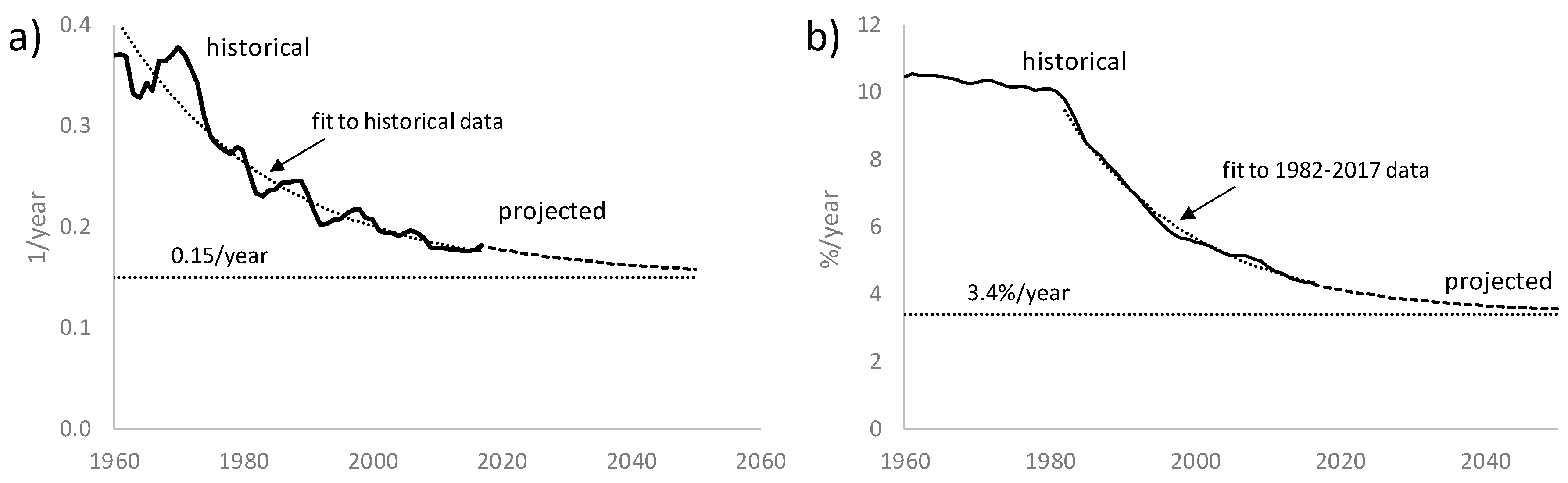
Second, we link capital stock to GDP using a constant capital productivity, and we assume a constant depreciation rate. Neither of these assumptions is strictly true (see Figure 2). However, for both parameters, a fit to the historical data is consistent with a gradual approach toward asymptotic values. Extrapolating those trends and taking the average over the scenario period (2017 to 2050) gives an average capital productivity of 0.17 per year and an average depreciation rate of 3.8% per year.
We initialize GDP to the 2017 value of Bds$9.35 billion (from the World Bank World Development Indicators database). Over the five-year period 2014–2018, the mean sea surface temperature anomaly was τ = 0.53 °C, corresponding to µ = 63.5 mph. We adopt that as the starting value.
3. Results
We built the model described above as a system dynamics model in Vensim. (Code is available from the authors upon request; the model requires Vensim DSS.) We ran three scenarios: stationary (a stationary climate); non-stationary no anticipation (non-stationary climate but a design threshold that does not anticipate any climate change); and non-stationary with anticipation (non-stationary climate with accurate anticipation of future climate). We note that a further (and arguably far more likely) scenario is a non-stationary climate in which climate change is anticipated, but inaccurately. However, the scenarios we have chosen are sufficient for the purpose of this paper, which is both to demonstrate the model and to explore whether anticipatory behavior (or lack of it) can substantially affect both adaptation costs and loss and damage.
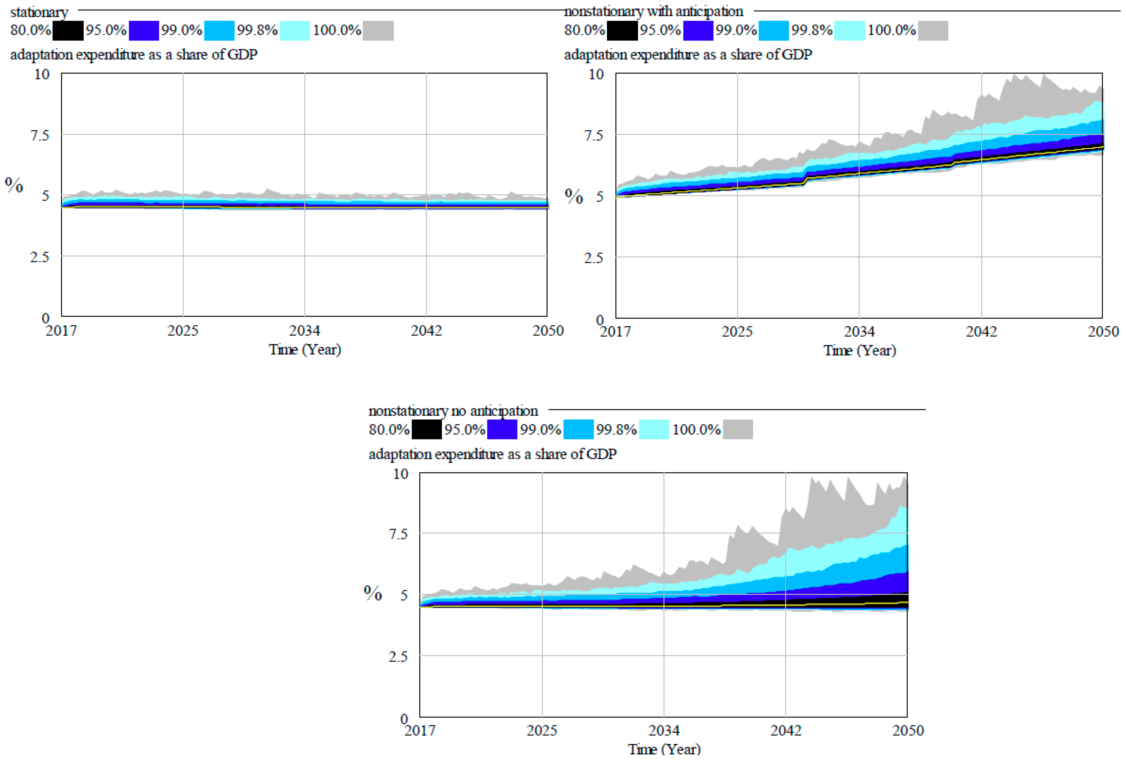
Each scenario was run from 2017 to 2050 in Monte Carlo mode, with storm parameters drawn from a GEV distribution. For the temperature anomaly we used trends from MAGICC/SCENGEN 5.3 [67] (which reports global average temperature rather than sea surface temperature) with the “no policy” P50 scenario. We adopted a piecewise linear rate of increase with breaks in 2030 and 2040, from 0.53 °C in 2017, to 0.85 °C in 2030, 1.17 °C in 2040, and 1.52 °C in 2050. Because storms represent extreme events, it takes a very large number of runs to generate a representative distribution. However, a smaller number of runs is sufficient to give an idea of trends. We ran each scenario 10,000 times, using the same pseudo-random number sequence for each scenario. The results are shown in the figures below. In each figure, the bands correspond, under stationary conditions, to 5-year return events (80%), 20-year events (95%), 100-year events (99%), and 500-year events (99.8%). In addition, the outer boundary for all events (100%) is shown. The mean value is shown as a yellow line.
Figure 3 shows adaptation expenditure as a share of GDP in the three scenarios. In the stationary scenario, even at the 99.8% level, adaptation expenditure remains below 5% of GDP. It rises through anticipatory behavior in the non-stationary with anticipation scenario. In the non-stationary no anticipation scenario, delays in rebuilding lead to a fall in GDP in the more extreme scenarios, so although costs are the same as in the stationary case, they rise as a share of GDP.
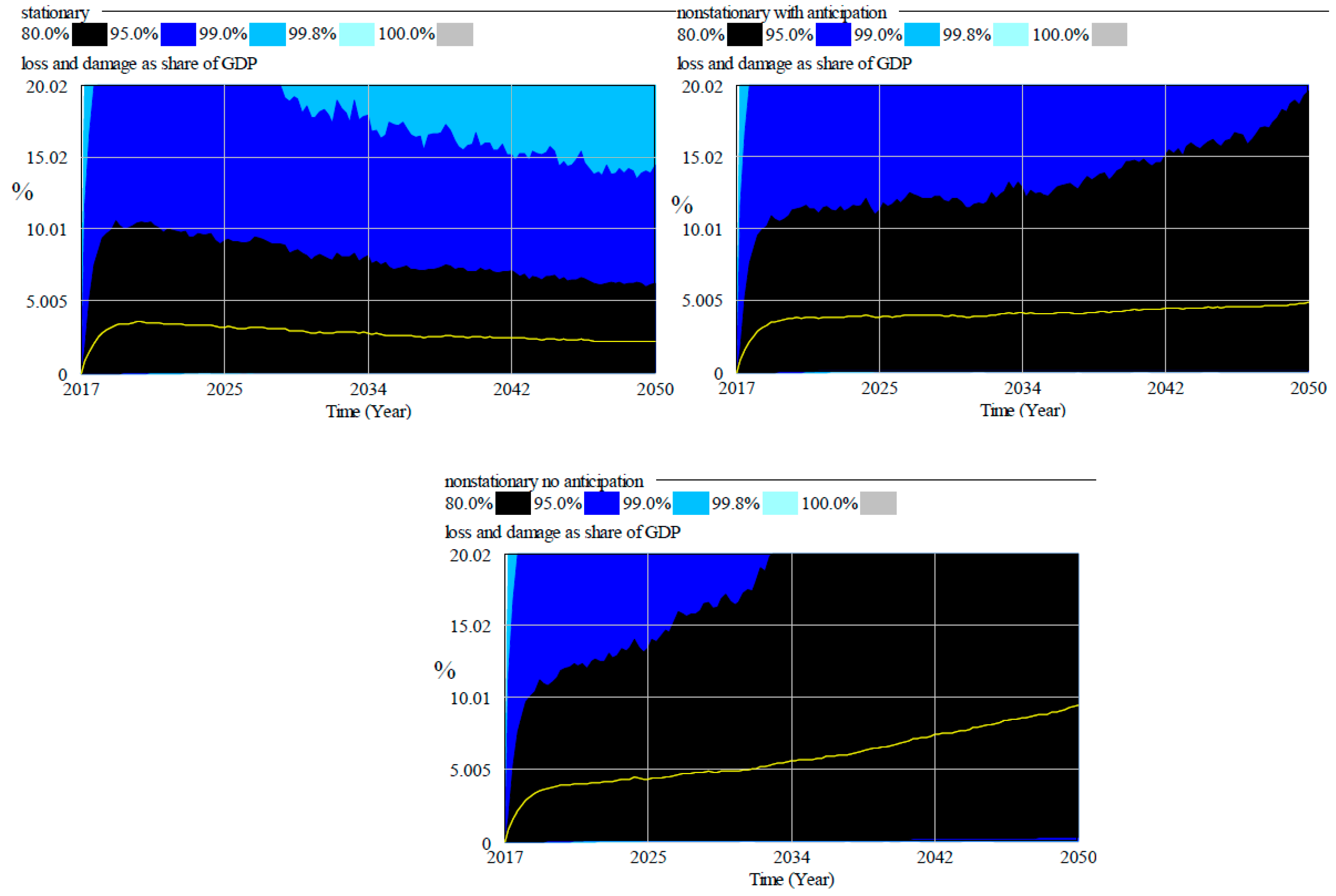
Figure 4 shows loss and damage expenditure as a share of GDP in the three scenarios. Following the model assumptions, loss and damage expenditure in any given year is capped at 20% of GDP, so repairs may take several years to complete. (The backlog of damaged capital starts at zero, giving the discontinuity in the graph in the first years.) Under stationary conditions, mean loss and damage is around 3% of GDP, and in 80% of cases loss and damage expenditure is below 10% of GDP, but due to the accumulation of a backlog, there is a good chance that expenditure can be higher. In at least 1% of cases (that is, 100–99%), it reaches the maximum level. Note that total damage will be even higher than is shown in the graph because the model does not take into account the duration of the storm and only tracks damage to productive capital stocks. Damage to houses, crops, municipal buildings, public infrastructure, and so on is not accounted for.
The difference between anticipation of climate change and building in line with historical climate change can be clearly seen in the non-stationary scenarios in Figure 4. The optimal design threshold trades off anticipated damage against mitigation cost, so damages rise in both non-stationary scenarios, with damage at the 95% (or 20-year) level overwhelming the capacity to rebuild in both scenarios. Yet, mean loss and damage expenditure rises only slightly in the non-stationary with anticipation scenario, while it rises substantially in the non-stationary no anticipation scenario.
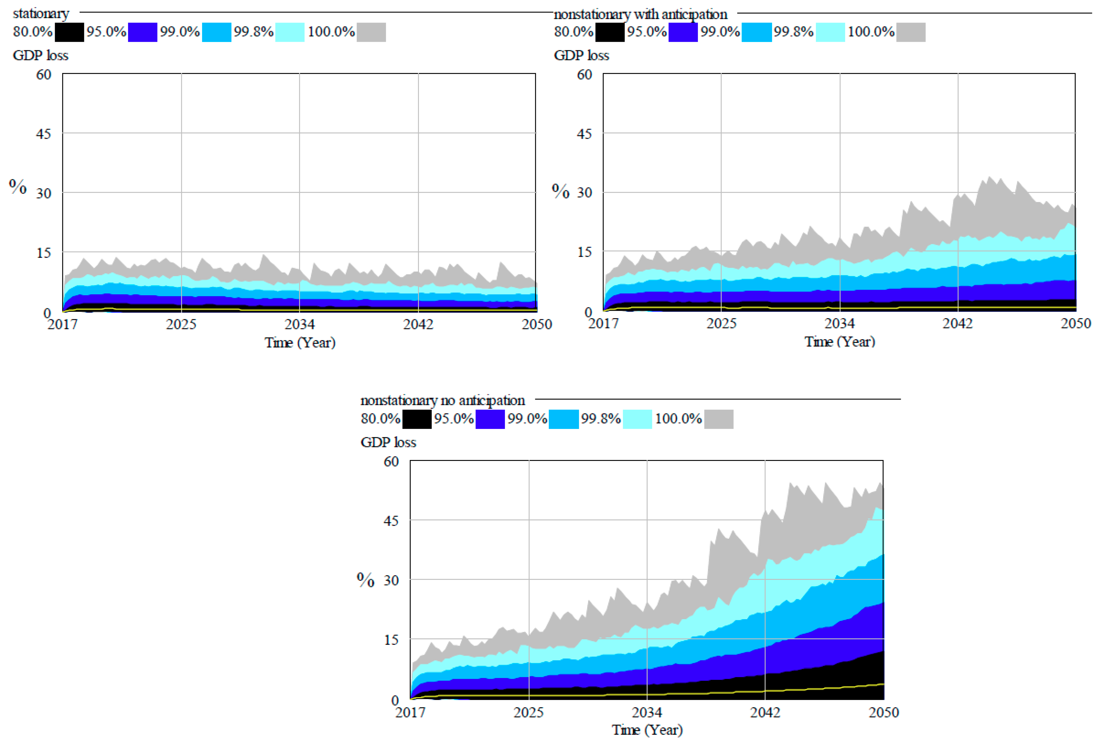
IAMs report damage as a GDP loss. For purposes of comparison, we calculated the loss relative to a baseline in which GDP grows at a steady rate of 2.7% per year. The results are shown in Figure 5. The mean values are comparatively small in the stationary and non-stationary with anticipation scenarios (less than 1.0% of GDP) because damaged capital is rebuilt, and the investment expenditure is part of GDP. These values are higher than the 0.2% per year estimated by Acevedo [33] and the study of Moore et al. [6], which found output losses for Barbados between 0.20% and 0.25% of GDP in 2050. This is because the model tracks a backlog of unrepaired damaged capital stocks, and cumulative damage increases subsequent GDP losses (see the discussion in [19]). Without anticipation, mean losses are higher still, on the order of 4% by 2050. Moreover, due to cumulative damage and the rebuilding backlog, even with anticipation there is a significant probability of greater losses, as shown by the rise in the 80% and 95% confidence intervals.
Consumption expenditures, and, therefore, living standards, are reduced because of expenditure for mitigation and loss & damage as well as from lower output due to damaged capital stocks. This is shown in Figure 6. In a stationary climate, even the most severe storms reduce consumption by no more than 0.5 percentage points of GDP. In a non-stationary climate, consumption losses can be substantial even when climate change is anticipated. We emphasize again that while our model includes forward-looking actors, they are not the social planners of the IAMs. Rather, they are engineers who attempt a minimum-cost design given their expectations of climate change at the time of construction. IAMs seek to maximize social welfare, which is normally taken to be an increasing function of household consumption. Thus, an IAM might produce a scenario with lower consumption losses and higher adaptation costs compared to the non-stationary with anticipation scenario that we present in this paper.
4. Discussion
We drew on standard methods in engineering risk assessment to develop a model for damage to commercial productive capital in the small island state of Barbados. Detailed impact models like ours are often used for local studies; such studies inform the damage functions used in the FUND model [9]. However, to our knowledge there is no bottom-up macroeconomic model that includes damage to productive capital. The closest we have found are the papers of Fankhauser and Tol [26], which introduced a temperature-dependent depreciation rate into different types of neoclassical growth models; and of Rezai et al. [10], which applied a greenhouse gas concentration-dependent depreciation rate in a post-Keynesian model.
The behaviorally-based damage model presented in this paper allows for greater flexibility than do temperature-dependent damage functions. Anticipating a changing climate or designing for current conditions produce different effective depreciation rates for the same change in global temperature, in contrast to Fankhauser and Tol [26], Moore et al. [6], or Rezai et al. [10]. Firms may rebuild damaged capital (as assumed in this paper) or suffer an extended loss of output. They may target a particular rate of growth, while damage costs are made up through lower consumption (as in this paper and FUND) or damages may be reflected in lower output and correspondingly lower saving and investment (as in DICE and Fankhauser and Tol [26]).
The simulation results presented in this paper provide a counterpoint to the climate damage models used in integrated assessment models. When running IAMs in an optimizing mode, the results are highly dependent on an assumed social discount rate [68,69,70,71,72,73]. The analysis in IAMs is normative: the investment trajectory maximizes social utility, taken to be an increasing function of consumption. In contrast, in this paper the analysis is descriptive. The discount rate is one that might be used by a private firm deciding between different investments. The simulation results produced by the model can be reviewed and critically assessed, and policy instruments chosen to make a socially desirable outcome more likely. For example, we assumed that capital of a given vintage would be rebuilt to its original specifications. Instead, it could be built to specifications of new investment, thus following the recommendation to “build back better” [74]. Alternatively, sufficiently extensive damage could lead to abandonment and migration [75]. Additional behavioral extensions could include insurance against climate damage and publicly-funded recovery efforts in the calculation of total costs in Equation (12).
A further contrast is between the use of specific moments of distributions (such as the mean) and a full distribution, as shown above in the model outputs. The importance of looking at the full distribution in climate damage studies was urged by Weitzman [69,76]. IAMs, when run in an optimizing mode, assume that agents choose an optimal expected future path over which expectations are calculated as the mean across different possible future states. The results in this paper make clear how misleading mean values can be when distributions are asymmetrical and have broad tails. In Figure 5, when climate damage is anticipated, mean GDP losses rise only slightly over the current value. However, losses at the 95% level (corresponding in the stationary case to a 20-year event) roughly double by 2050, suggesting a substantial probability of hardship arising from storm damage.
5. Conclusions
The dominant approach to computing climate damages in economic models is to use a temperature-dependent damage function. This has some advantages at global level, where damage estimates are aggregates over highly heterogeneous local impacts. However, they are less appropriate for local studies, where a wide variety of modelled climate variables may be available, such as the frequencies of extreme climate events, and it is possible and relevant to explore alternative behavioral assumptions.
Local studies are particularly needed for small island developing states (SIDS), which must contend with the compound uncertainties of heavy reliance on export markets and potentially rising climate damage. SIDS rely on capital-intensive export industries, and both the capital stocks and transport costs can be affected by tropical cyclones.
In this paper we drew upon the literature on engineering design and risk assessment to develop a model for damage to commercial productive capital and applied it to the small island state of Barbados. The model features behavioral variables that are not captured by temperature-dependent damage functions, such as anticipation of future climate change. We found that anticipatory behavior can substantially affect climate impacts on the economy.
Author Contributions
Conceptualization, E.K.-B. and J.L.; formal analysis, E.K.-B., J.L., and T.L.; funding acquisition, E.K.-B.; investigation, E.K.-B. and C.D.; methodology, E.K.-B. and J.L.; project administration, E.K.-B.; writing—original draft, E.K.-B., J.L., T.L., and C.D.; writing—review and editing, E.K.-B., J.L., T.L., and C.D.
Funding
The work presented in this paper was funded in part by the Stockholm Environment Institute from funds provided by the Swedish International Development Cooperation Agency (Sida). It substantially extends earlier work carried out under the Global to Local Caribbean Climate Change Adaptation and Mitigation Scenarios (GoLoCarSce) and the Sustainable Water Management under Climate Change in Small Island States of the Caribbean (Water-aCCIS) research projects. GoLoCarSce was funded by the European Union African, Caribbean and Pacific (ACP) Research Programme for Sustainable Development (CP-RSD, Contract Number FED/2011/281-134). The funding for Water-aCCIS was provided by the International Development Research Centre (IDRC, Grant 107096-001). The results can under no circumstances be regarded as reflecting the position of Sida, the European Union, or IDRC.
Acknowledgments
The authors would like to thank John Agard and Adrian Cashman for their guidance on the GoLoCarSce and Water-aCCIS projects, which provided the foundation for the work presented here, and for their encouragement to build on that foundation in the writing of this paper.
Conflicts of Interest
The authors declare no conflict of interest. The funders had no role in the design of the study; in the collection, analyses, or interpretation of data; in the writing of the manuscript; or in the decision to publish the results.
Appendix A. Estimating Parameters for the Wind Speed Model
Data on storms for the Eastern Caribbean extends from 1851 to 2010, while that for Barbados extends from 1855 to 2010. We note that a bias in historical data identified by Landsea [77] appears to have been corrected in the HURDAT database [78]. Thus, in contrast to Acevedo [33], we do not adjust historical wind speeds. For three out of 58 storms that reached Barbados, the peak wind speed recorded in Barbados exceeded that recorded for the Eastern Caribbean. Since Barbados is part of the Eastern Caribbean, we considered those to be recording errors and set the ratios equal to one. Otherwise, we used the ratio of the recorded peak wind speed in the Eastern Caribbean to that in Barbados. The average ratio, which is our parameter ϕ, we found to be 1.34, with a standard deviation of 0.41. This parameter is comparatively stable over time, despite an apparent rising trend. A one-sided, two-sample, Wilcoxon rank sum test for whether the mean before 1931 (the median year for storms in Barbados) is lower than after 1931 could not reject the null hypothesis of no difference between the means (p = 0.41).
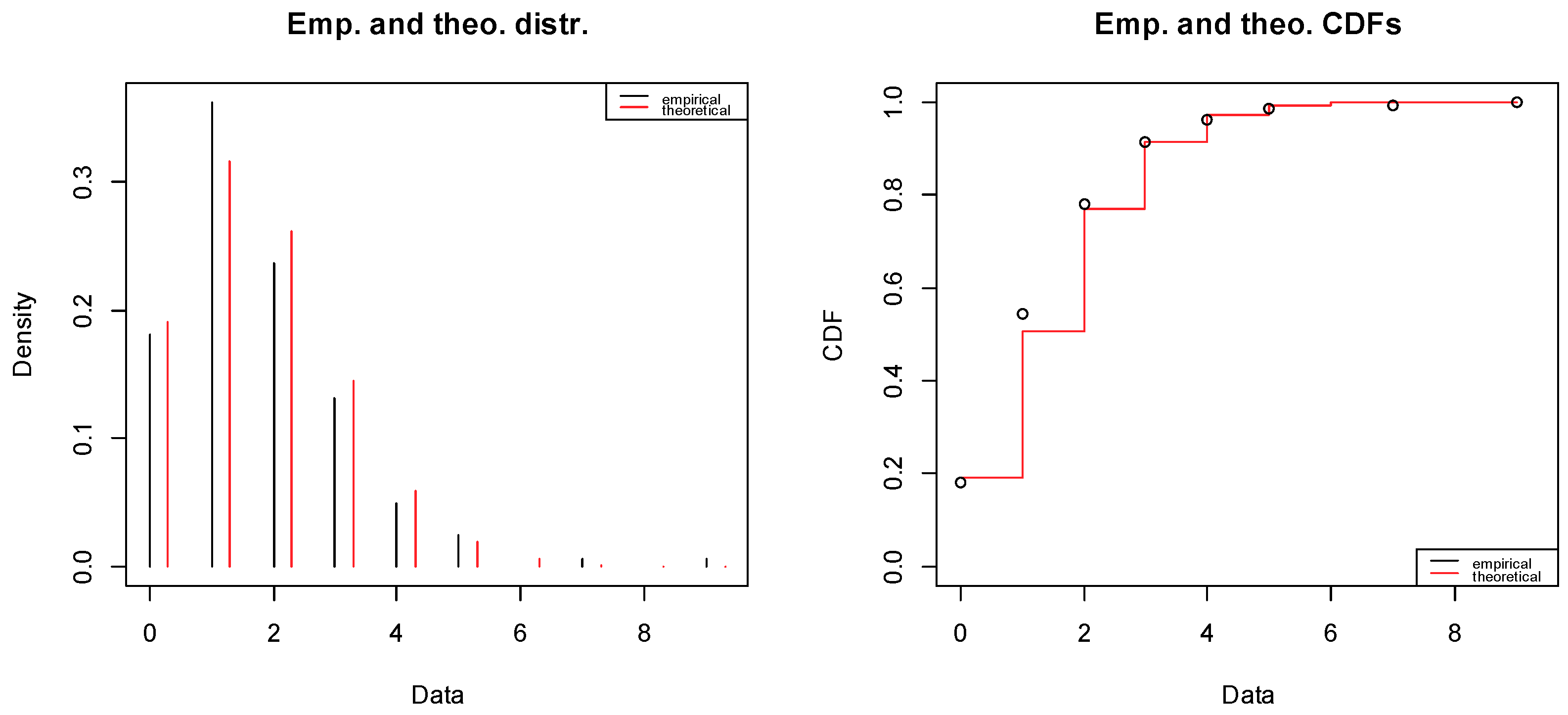
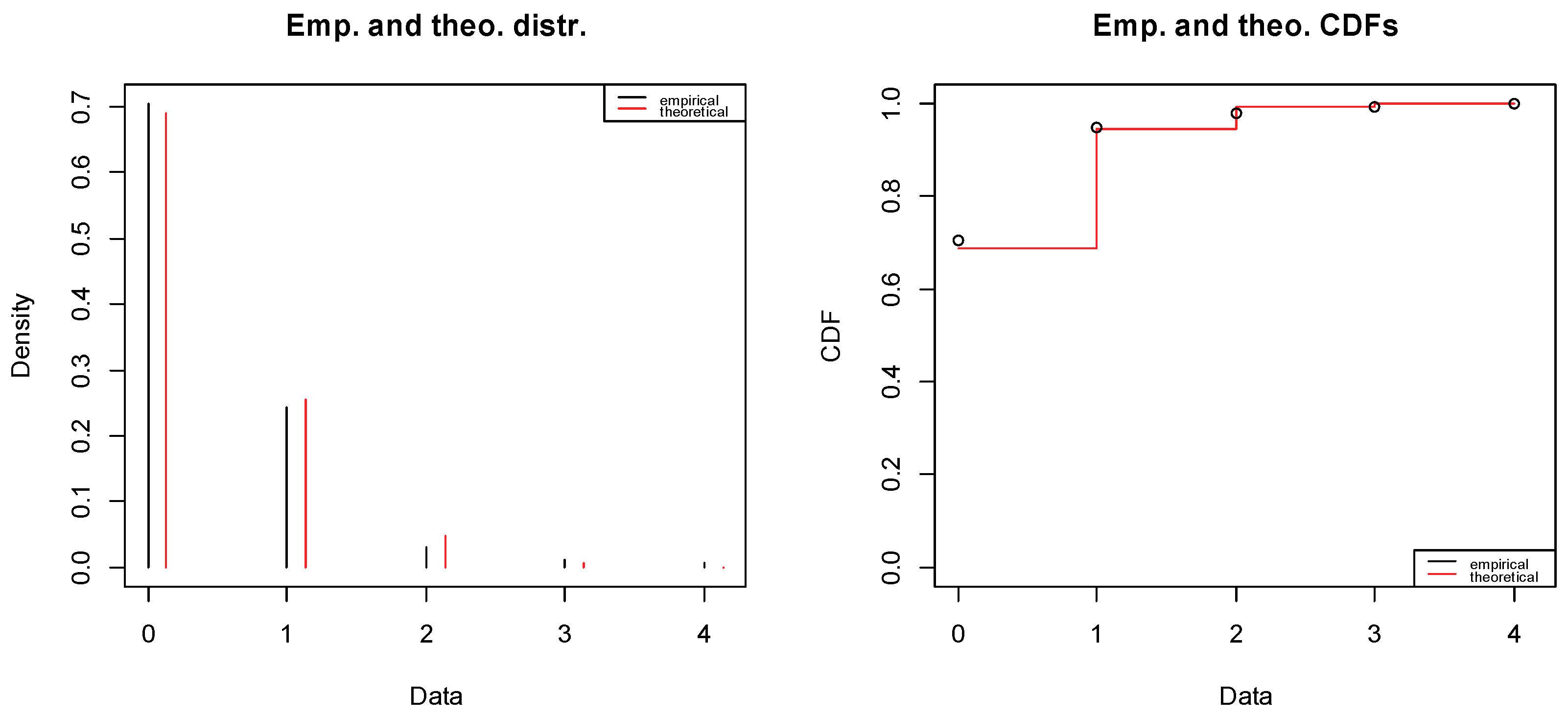
We used count data of storms per year to estimate a Poisson model for storms with a peak wind speed of at least 40 mph (using the R fitdistrplus package ver. 1.0-11) for both the Eastern Caribbean and Barbados. Graphical representations of the fit for the Eastern Caribbean are shown in Figure A1 and for Barbados in Figure A2. The parameter estimate for the Eastern Caribbean is λ = 1.56 ± 0.20 (to two standard deviations), corresponding to a return period of 1.24 years, and for Barbados λ = 0.37 ± 0.10, corresponding to a return period of 3.22 years. To estimate the strike probability in Equation (21), we computed a Poission fit for the Eastern Caribbean for storms with wind speed wt = ϕ × 40.0 mph = 53.6 mph and compared the exceedance probability to that of a 40-mph storm in Barbados. The result is ps = 0.36.
Figure A1.
Poisson distribution fit for storm events in the Eastern Caribbean.

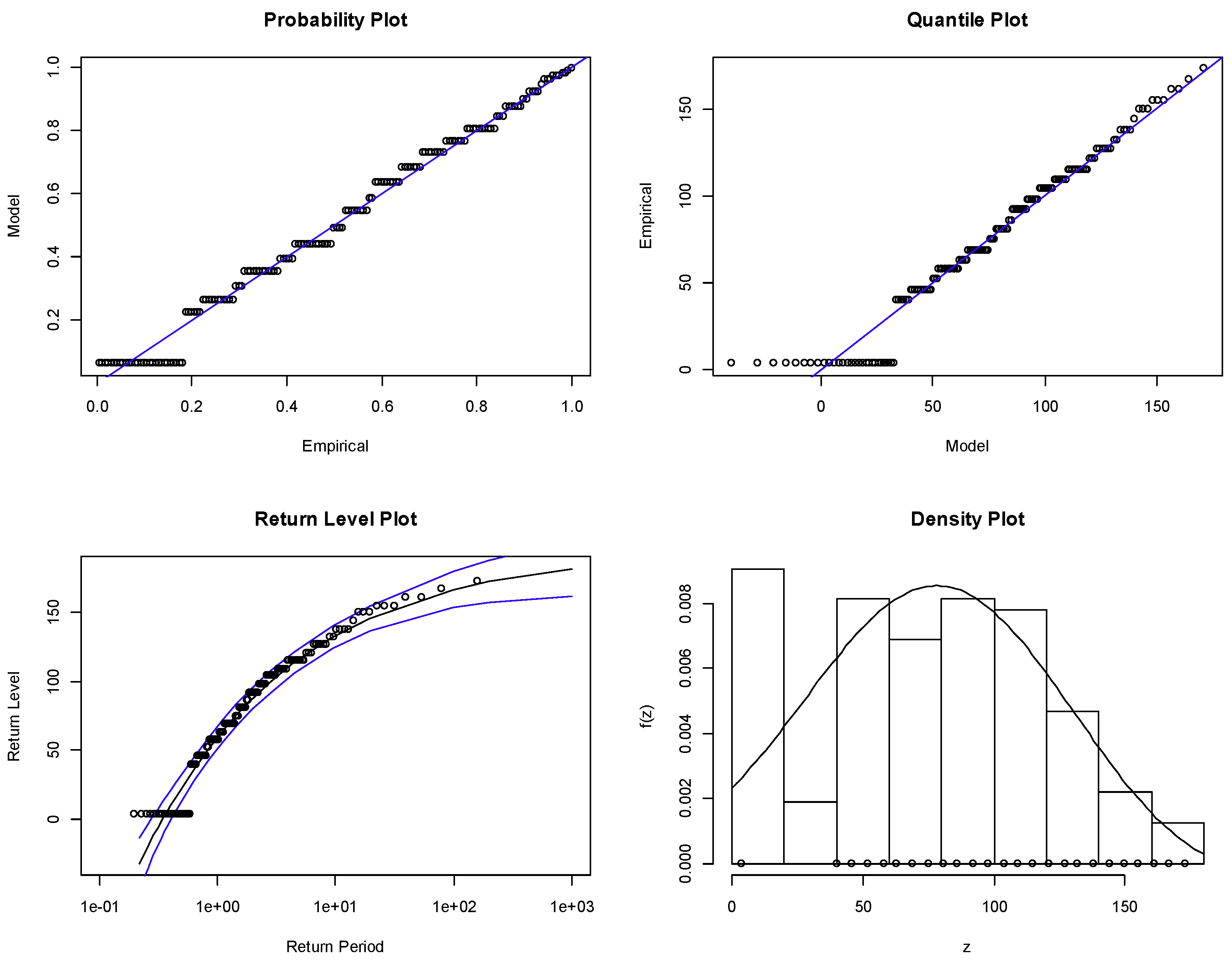
Next, we selected the peak wind speed in each year for the Eastern Caribbean. Wind speeds are not recorded for years without storms. Thus, there is no data for years when peak wind speed data fell below 40 mph, the minimum for a tropical storm. In those years we set the peak wind speed to a common value—the mean below the threshold—and fit a stationary GEV distribution (using the R package ismev ver. 1.42) that is truncated to the left at x = 0. We found the mean value below the threshold in an iterative procedure in which we: initialized the mean below threshold to one-half the threshold, fit the GEV, calculated the mean below the threshold with the fitted parameters, used that value for the next iteration, and iterated until the estimated mean below threshold converged to a tolerance of 10−7 mph. This procedure found an estimated mean (non-storm) peak wind speed below threshold of 3.74 mph.
Figure A2.
Poisson distribution fit for storm events in Barbados.

Diagnostic plots for the fitted GEV distribution are shown in Figure A3. As shown in the figure, the full GEV parameter set is needed to capture the behavior at high wind speeds (i.e., a Gumbel distribution would be inappropriate). The estimated parameters for the Eastern Caribbean are μEC = 60.1 ± 8.1 mph, σEC = 46.0 ± 5.9 mph, ξEC = –0.34 ± 0.11 (again to two standard deviations). This corresponds to a return period of 1.29 years for storms with the threshold peak wind speed (40 mph), in reasonable agreement with the Poisson estimate of 1.24 years.
Figure A3.
Diagnostic plots for storm data in the Eastern Caribbean as a stationary generalized extreme value (GEV).
Figure A3.
Diagnostic plots for storm data in the Eastern Caribbean as a stationary generalized extreme value (GEV).

For the non-stationary GEV model we used as a covariate the global average sea surface temperature anomaly, τ, relative to the 1961–1990 average from the Hadley Climate Research Unit (https://www.metoffice.gov.uk/hadobs/). The justification is provided in the main text. Sea surface temperature does not drive non-storm peak wind speeds, so we expect peak wind speeds in the upper part of the distribution to be more sensitive to sea surface temperature than in the lower part. Consistent with this assumption, Elsner et al. [79] found the upper quintiles of peak tropical storm wind speed to rise over time and with changing sea surface temperature, but not the lower quintiles. Accordingly, for this fit we again set the peak wind speed for years with no data to 3.74 mph, the value that we estimated for the stationary distribution.
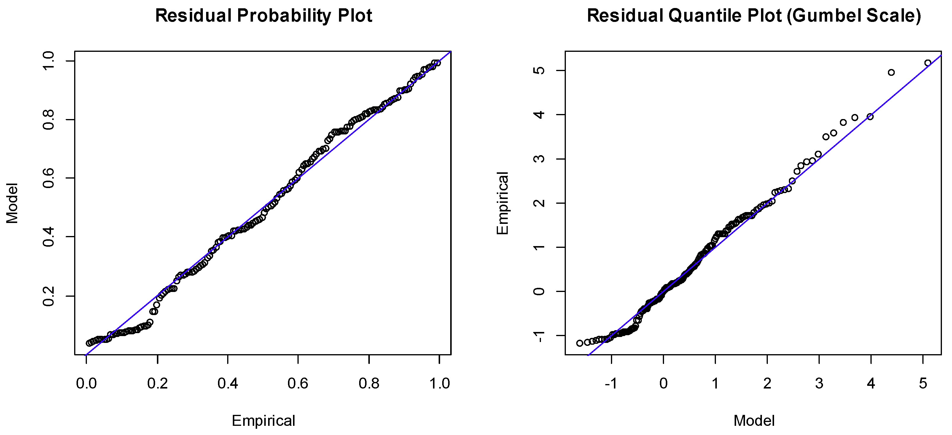
Only the location parameter had a statistically significant correlation to sea surface temperature at the 5% level. Setting up a model with a temperature-dependent location parameter, the residual probability and quantile plots are shown in Figure A4. The estimated parameters are μEC = (65.6 + 36.7 τ) ± (9.1 + 29.7 τ) mph, σEC = 45.9 ± 6.1 mph, ξEC = –0.37 ± 0.12.
Figure A4.
Diagnostic plots for the non-stationary GEV distribution.

References
- Nicholls, R.J.; Tol, R.S.J. Impacts and responses to sea-level rise: A global analysis of the SRES scenarios over the twenty-first century. Philos. Trans. R. Soc. A Math. Phys. Eng. Sci. 2006, 364, 1073–1095. [Google Scholar] [CrossRef] [PubMed]
- Nurse, L.A.; McLean, R.F.; Agard, J.; Briguglio, L.P.; Duvat-Magnan, V.; Pelesikoti, N.; Tompkins, E.; Webb, A. Small islands. In Climate Change 2014: Impacts, Adaptation, and Vulnerability. Part B: Regional Aspects. Contribution of Working Group II to the Fifth Assessment Report of the Intergovernmental Panel of Climate Change; Barros, V.R., Field, C.B., Dokken, D.J., Mastrandrea, M.D., Mach, K.J., Bilir, T.E., Chatterjee, M., Eds.; Cambridge University Press: Cambridge, UK; New York, NY, USA, 2014; pp. 1613–1654. [Google Scholar]
- William, E.; Kraay, A. Small States, Small Problems? SSRN Scholarly Paper ID 620631; Social Science Research Network: Rochester, NY, USA, 1999. [Google Scholar]
- Armstrong, H.W.; Read, R. The phantom of liberty? Economic growth and the vulnerability of small states. J. Int. Dev. 2002, 14, 435–458. [Google Scholar] [CrossRef]
- Kemp-Benedict, E.; Drakes, C.; Laing, T. Export-led growth, global integration, and the external balance of small island developing states. Economies 2018, 6, 35. [Google Scholar] [CrossRef]
- Moore, W.; Elliott, W.; Lorde, T. Climate change, Atlantic storm activity and the regional socio-economic impacts on the Caribbean. Environ. Dev. Sustain. 2016, 19, 707–726. [Google Scholar] [CrossRef]
- Nordhaus, W.D. Rolling the ‘DICE’: An optimal transition path for controlling greenhouse gases. Resour. Energy Econ. 1993, 15, 27–50. [Google Scholar] [CrossRef]
- Nordhaus, W.D. Revisiting the social cost of carbon. Proc. Natl. Acad. Sci. USA 2017, 114, 1518–1523. [Google Scholar] [CrossRef] [PubMed] [Green Version]
- Anthoff, D.; Tol, R.S.J. The Climate Framework for Uncertainty, Negotiation and Distribution (FUND): Technical Description, Version 3.6; Forschungsstelle für Nachhaltige Entwicklung, Universität Hamburg: Hamburg, Germany, 2012. [Google Scholar]
- Rezai, A.; Taylor, L.; Foley, D. Economic growth, income distribution, and climate change. Ecol. Econ. 2018, 146, 164–172. [Google Scholar] [CrossRef]
- Edmonds, J.A.; Wise, M.A.; MacCracken, C.N. Advanced Energy Technologies and Climate Change: An Analysis Using the Global Change Assessment Model (GCAM); PNL-9798; Pacific Northwest National Lab. (PNNL): Richland, WA, USA, 1994. [Google Scholar]
- Kim, S.H.; Edmonds, J.; Lurz, J.; Smith, S.J.; Wise, M. The objects framework for integrated assessment: Hybrid modeling of transportation. Energy J. 2006, 27, 63–91. [Google Scholar] [CrossRef]
- Bréchet, T.; Camacho, C.; Veliov, V.M. Adaptive model-predictive climate policies in a multicountry setting. In The Oxford Handbook of the Macroeconomics of Climate Change; Bernard, L., Semmler, W., Eds.; Oxford University Press: Oxford, UK, 2015; pp. 114–138. [Google Scholar]
- Tol, R.S.J. Estimates of the damage costs of climate change. Part I: Benchmark estimates. Environ. Resour. Econ. 2002, 21, 47–73. [Google Scholar] [CrossRef]
- Tol, R.S.J. Estimates of the damage costs of climate change. Part II. Dynamic estimates. Environ. Resour. Econ. 2002, 21, 135–160. [Google Scholar] [CrossRef]
- Taylor, L. Reconstructing Macroeconomics: Structuralist Proposals and Critiques of the Mainstream; Harvard University Press: Cambridge, MA, USA, 2004. [Google Scholar]
- Ocampo, J.A.; Rada, C.; Taylor, L. Growth and Policy in Developing Countries: A Structuralist Approach; Columbia University Press: New York, NY, USA, 2009. [Google Scholar]
- Donadelli, M.; Jüppner, M.; Riedel, M.; Schlag, C. Temperature shocks and welfare costs. J. Econ. Dyn. Control 2017, 82, 331–355. [Google Scholar] [CrossRef]
- Piontek, F.; Kalkuhl, M.; Kriegler, E.; Schultes, A.; Leimbach, M.; Edenhofer, O.; Bauer, N. Economic growth effects of alternative climate change impact channels in economic modeling. Env. Resour. Econ. 2018. [Google Scholar] [CrossRef]
- Strobl, E. The economic growth impact of natural disasters in developing countries: Evidence from hurricane strikes in the Central American and Caribbean regions. J. Dev. Econ. 2012, 97, 130–141. [Google Scholar] [CrossRef]
- Hallegatte, S.; Rozenberg, J. Climate change through a poverty lens. Nat. Clim. Chang. 2017, 7, 250–256. [Google Scholar] [CrossRef]
- Strobl, E. The economic growth impact of hurricanes: Evidence from U.S. coastal counties. Rev. Econ. Stat. 2011, 93, 575–589. [Google Scholar] [CrossRef]
- Noy, I. The macroeconomic consequences of disasters. J. Dev. Econ. 2009, 88, 221–231. [Google Scholar] [CrossRef] [Green Version]
- IPCC. Managing the Risks of Extreme Events and Disasters to Advance Climate Change Adaptation; Field, C.B., Barros, V., Stocker, T.F., Qin, D., Dokken, D.J., Ebi, K.L., Mastrandrea, M.D., Mach, K.J., Plattner, G.-K., Allen, S.K., et al., Eds.; No. A Special Report of the Intergovernmental Panel on Climate Change Working Groups I and II; Cambridge University Press: Cambridge, UK; New York, NY, USA, 2012. [Google Scholar]
- USGCRP. Fourth National Climate Assessment, Volume II: Impacts, Risks, and Adaptation in the United States; Reidmiller, D.R., Avery, C.W., Easterling, D.R., Kunkel, K.E., Lewis, K.L.M., Maycock, T.K., Stewart, B.C., Eds.; U.S. Global Change Research Program: Washington, DC, USA, 2018. [Google Scholar]
- Fankhauser, S.; Tol, R.S.J. On climate change and economic growth. Resour. Energy Econ. 2005, 27, 1–17. [Google Scholar] [CrossRef]
- Hirabayashi, Y.; Mahendran, R.; Koirala, S.; Konoshima, L.; Yamazaki, D.; Watanabe, S.; Kim, H.; Kanae, S. Global flood risk under climate change. Nat. Clim. Chang. 2013, 3, 816–821. [Google Scholar] [CrossRef]
- Lin, N.; Kopp, R.E.; Horton, B.P.; Donnelly, J.P. Hurricane Sandy’s flood frequency increasing from year 1800 to 2100. Proc. Natl. Acad. Sci. USA 2016, 113, 12071–12075. [Google Scholar] [CrossRef]
- Stedinger, J.R.; Vogel, R.M.; Foufoula-Georgiou, E. Frequency analysis of extreme events. In Handbook of Hydrology; Maidment, D.R., Ed.; McGraw-Hill: New York, NY, USA, 1993. [Google Scholar]
- Vogel, R.M.; Castellarin, A. Risk, reliability, and return periods and hydrologic design. In Handbook of Applied Hydrology; Singh, V.P., Ed.; McGraw-Hill Book Company: New York, NY, USA, 2017. [Google Scholar]
- Organization of American States. Primer on Natural Hazard Management in Integrated Regional Development Planning; Organization of American States: Washington, DC, USA, 1991. [Google Scholar]
- Economic Commission for Latin America and the Caribbean. An Assessment of the Economic and Social Impacts of Climate Change on the Health Sector in the Caribbean; Economic Commission for Latin America and the Caribbean, United Nations: Port of Spain, Trinidad and Tobago, 2011. [Google Scholar]
- Acevedo, S. Gone with the Wind: Estimating Hurricane and Climate Change Costs in the Caribbean; IMF Working Papers; IMF: Washington, DC, USA, 2016; Volume 16, p. 1. [Google Scholar]
- Sheehan, M. Hurricanes Harvey, Irma, and Maria Cost Re/Insurers $80bn: Impact Forecasting. Reinsurance News, 5 April 2018. [Google Scholar]
- Ötker, I.; Srinivasan, S. Bracing for the storm. For the Caribbean building resilience is a matter of survival. Financ. Dev. 2018, 55, 1. [Google Scholar]
- Langbein, W.B. Annual floods and the partial-duration flood series. Eos Trans. Am. Geophys. Union 1949, 30, 879–881. [Google Scholar] [CrossRef]
- Rogger, M.; Agnoletti, M.; Alaoui, A.; Bathurst, J.C.; Bodner, G.; Borga, M.; Chaplot, V.; Gallart, F.; Glatzel, G.; Hall, J.; et al. Land use change impacts on floods at the catchment scale: Challenges and opportunities for future research. Water Resour. Res. 2017, 53, 5209–5219. [Google Scholar] [CrossRef] [PubMed] [Green Version]
- Milly, P.C.D.; Betancourt, J.; Falkenmark, M.; Hirsch, R.M.; Kundzewicz, Z.W.; Lettenmaier, D.P.; Stouffer, R.J. Stationarity is dead: Whither water management? Science 2008, 319, 573–574. [Google Scholar] [CrossRef] [PubMed]
- Serinaldi, F.; Kilsby, C.G. Stationarity is undead: Uncertainty dominates the distribution of extremes. Adv. Water Resour. 2015, 77, 17–36. [Google Scholar] [CrossRef] [Green Version]
- Salas, J.D.; Obeysekera, J. Revisiting the concepts of return period and risk for nonstationary hydrologic extreme events. J. Hydrol. Eng. 2014, 19, 554–568. [Google Scholar] [CrossRef]
- Read, L.K.; Vogel, R.M. Reliability, return periods, and risk under nonstationarity. Water Resour. Res. 2015, 51, 6381–6398. [Google Scholar] [CrossRef]
- Vogel, R.M.; Yaindl, C.; Walter, M. Nonstationarity: Flood magnification and recurrence reduction factors in the United States. JAWRA J. Am. Water Resour. Assoc. 2011, 47, 464–474. [Google Scholar] [CrossRef]
- McKenzie, R.; Levendis, J. Flood hazards and urban housing markets: The effects of Katrina on New Orleans. J. Real Estate Financ. Econ. 2010, 40, 62–76. [Google Scholar] [CrossRef]
- Feenstra, R.C.; Inklaar, R.; Timmer, M.P. The next generation of the Penn World Table. Am. Econ. Rev. 2015, 105, 3150–3182. [Google Scholar] [CrossRef]
- Ambler, S.; Paquet, A. Stochastic depreciation and the business cycle. Int. Econ. Rev. 1994, 35, 101–116. [Google Scholar] [CrossRef]
- Dueker, M.; Fischer, A.; Dittmar, R. Stochastic capital depreciation and the co-movement of hours and productivity. B.E. J. Macroecon. 2007, 6. [Google Scholar] [CrossRef]
- Furlanetto, F.; Seneca, M. New perspectives on depreciation shocks as a source of business cycle fluctuations. Macroecon. Dyn. 2014, 18, 1209–1233. [Google Scholar] [CrossRef]
- Fankhauser, S.; Smith, J.B.; Tol, R.S.J. Weathering climate change: Some simple rules to guide adaptation decisions. Ecol. Econ. 1999, 30, 67–78. [Google Scholar] [CrossRef]
- Pindyck, R.S. Climate change policy: What do the models tell us? J. Econ. Lit. 2013, 51, 860–872. [Google Scholar] [CrossRef]
- Blank, L.; Tarquin, A. Engineering Economy, 8th ed.; McGraw-Hill Education: New York, NY, USA, 2018. [Google Scholar]
- Baum, S.D. Description, prescription and the choice of discount rates. Ecol. Econ. 2009, 69, 197–205. [Google Scholar] [CrossRef] [Green Version]
- Weitzman, M.L. Gamma discounting. Am. Econ. Rev. 2001, 91, 260–271. [Google Scholar] [CrossRef]
- Landsea, C.W.; Franklin, J.L. Atlantic hurricane database uncertainty and presentation of a new database format. Mon. Weather Rev. 2013, 141, 3576–3592. [Google Scholar] [CrossRef]
- Holland, G.J. The maximum potential intensity of tropical cyclones. J. Atmos. Sci. 1997, 54, 2519–2541. [Google Scholar] [CrossRef]
- Vecchi, G.A.; Soden, B.J. Effect of remote sea surface temperature change on tropical cyclone potential intensity. Nature 2007, 450, 1066–1070. [Google Scholar] [CrossRef]
- Donadelli, M.; Jüppner, M.; Paradiso, A.; Schlag, C. Temperature volatility risk. Ssrn Electron. J. 2019. [Google Scholar] [CrossRef]
- Zhai, A.R.; Jiang, J.H. Dependence of US hurricane economic loss on maximum wind speed and storm size. Environ. Res. Lett. 2014, 9, 064019. [Google Scholar] [CrossRef]
- Lin, N.; Emanuel, K.; Oppenheimer, M.; Vanmarcke, E. Physically based assessment of hurricane surge threat under climate change. Nat. Clim. Chang. 2012, 2, 462–467. [Google Scholar] [CrossRef] [Green Version]
- Unanwa, C.O.; McDonald, J.R.; Mehta, K.C.; Smith, D.A. The development of wind damage bands for buildings. J. Wind Eng. Ind. Aerodyn. 2000, 84, 119–149. [Google Scholar] [CrossRef]
- Vickery, P.J.; Skerlj, P.F.; Lin, J.; Twisdale, L.A.; Young, M.A.; Lavelle, F.M. HAZUS-MH hurricane model methodology. II: Damage and loss estimation. Nat. Hazards Rev. 2006, 7, 94–103. [Google Scholar] [CrossRef]
- Nordhaus, W.D. The economics of hurricanes and implications of global warming. Clim. Chang. Econ. 2010, 1, 1–20. [Google Scholar] [CrossRef]
- Bouwer, L.M.; Botzen, W.W.J. How sensitive are US hurricane damages to climate? Comment on a paper by W. D. Nordhaus. Clim. Chang. Econ. 2011, 2, 1–7. [Google Scholar] [CrossRef]
- Murphy, A.; Strobl, E. The Impact of Hurricanes on Housing Prices: Evidence from U.S. Coastal Cities; Federal Reserve Bank of Dallas, Working Papers; Federal Reserve Bank of Dallas: Dallas, TX, USA, 2010. [Google Scholar]
- USACE. Risk Assessment for Flood Risk Management Studies; Engineering Regulation USACE ER 1105-2-101; US Army Corps of Engineers: Washington, DC, USA, 2017. [Google Scholar]
- Miethe, J. Using Hurricanes to Uncover (Non-)Activity in Offshore Financial Centers; Job Market Paper; Humboldt University Berlin and German Institute of Economic Research (DIW Berlin): Berlin, Germany, 2019. [Google Scholar]
- Garcia-Bernardo, J.; Fichtner, J.; Takes, F.W.; Heemskerk, E.M. Uncovering offshore financial centers: Conduits and sinks in the global corporate ownership network. Sci. Rep. 2017, 7, 6246. [Google Scholar] [CrossRef]
- Fordham, D.A.; Wigley, T.M.L.; Watts, M.J.; Brook, B.W. Strengthening forecasts of climate change impacts with multi-model ensemble averaged projections using MAGICC/SCENGEN 5.3. Ecography 2012, 35, 4–8. [Google Scholar] [CrossRef]
- Tol, R.S.J. The marginal damage costs of carbon dioxide emissions: An assessment of the uncertainties. Energy Policy 2005, 33, 2064–2074. [Google Scholar] [CrossRef]
- Weitzman, M.L. On modeling and interpreting the economics of catastrophic climate change. Rev. Econ. Stat. 2009, 91, 1–19. [Google Scholar] [CrossRef]
- Ackerman, F.S.J.; DeCanio, R.B.H.; Sheeran, K. Limitations of integrated assessment models of climate change. Clim. Chang. 2009, 95, 297–315. [Google Scholar] [CrossRef] [Green Version]
- Kopp, R.E.; Golub, A.; Keohane, N.O.; Onda, C. The influence of the specification of climate change damages on the social cost of carbon. Econ. Open Access Open Assess. E-J. 2012, 6, 2012–2013. [Google Scholar] [CrossRef]
- Botzen, W.J.W.; van den Bergh, J.C.J.M. How sensitive is Nordhaus to Weitzman? Climate policy in DICE with an alternative damage function. Econ. Lett. 2012, 117, 372–374. [Google Scholar] [CrossRef]
- IPCC. Summary for policymakers. In Climate Change 2014: Impacts, Adaptation, and Vulnerability. Contribution of Working Group II to the Fifth Assessment Report of the Intergovernmental Panel on Climate Change; Field, C.B., Barros, V.R., Dokken, D.J., Mach, K.J., Mastandrea, M.D., Bilir, T.E., Chatterjee, M., Eds.; Cambridge University Press: Cambridge, UK; New York, NY, USA, 2014; pp. 1–32. [Google Scholar]
- Hallegatte, S.; Rentschler, J.; Walsh, B. 2018. Building Back Better: Achieving Resilience through Stronger, Faster, and More Inclusive Post-Disaster Reconstruction. Risk and Vulnerability Assessment; World Bank: Washington, DC, USA, 2018. [Google Scholar]
- Black, R.; Bennett, S.R.G.; Thomas, S.M.; Beddington, J.R. Climate change: Migration as adaptation. Nature 2011, 478, 447–449. [Google Scholar] [CrossRef] [PubMed]
- Weitzman, M.L. Fat-tailed uncertainty in the economics of catastrophic climate change. Rev. Environ. Econ. Policy 2011, 5, 275–292. [Google Scholar] [CrossRef]
- Landsea, C.W. A climatology of intense (or major) Atlantic hurricanes. Mon. Weather Rev. 1993, 121, 1703–1713. [Google Scholar] [CrossRef]
- Landsea, C.W.; Anderson, C.; Charles, N.; Clark, G.; Dunion, J.; Fernandez-Partagas, J.; Hungerford, P.; Neumann, C.; Zimmer, M. The Atlantic hurricane database re-analysis project: Documentation for the 1851–1910 alterations and additions to the HURDAT database. In Hurricanes and Typhoons: Past, Present and Future; Murnane, R.J., Liu, K.-B., Eds.; Columbia University Press: New York, NY, USA, 2004; pp. 177–221. [Google Scholar]
- Elsner, J.B.; Kossin, J.P.; Jagger, T.H. The increasing intensity of the strongest tropical cyclones. Nature 2008, 455, 92–95. [Google Scholar] [CrossRef]
Figure 1.
Hypothetical distribution and damage as functions of event magnitude. The average damage ratio can be computed as.
Figure 1.
Hypothetical distribution and damage as functions of event magnitude. The average damage ratio can be computed as.

Figure 2.
Capital productivity (a) and depreciation rate (b) for Barbados, historical and projected.
Figure 2.
Capital productivity (a) and depreciation rate (b) for Barbados, historical and projected.

Figure 3.
Adaptation expenditure as a share of GDP (as %) in the three scenarios.

Figure 4.
Loss and damage expenditure as a share of GDP (as %) in the three scenarios.

Figure 5.
Output losses (as %) relative to a steady growth path in the three scenarios.

Figure 6.
Consumption (as % of GDP) in the three scenarios.


Table 1.
Estimated and observed return periods for storms classified on the Saffir–Simpson scale.
| Return Period (years) | ||||
|---|---|---|---|---|
| Category | Threshold (mph) | GEV Estimate | Observed | Number of Observations |
| Tropical storm | 18 | 3 | 3 | 46 |
| CAT 1 | 74 | 9 | 13 | 6 |
| CAT 2 | 96 | 25 | 26 | 3 |
| CAT 3 | 111 | 82 | 52 | 3 |
| CAT 4 | 130 | 2594 | NA | 0 |
| CAT 5 | 157 | Infinite | NA | 0 |
© 2019 by the authors. Licensee MDPI, Basel, Switzerland. This article is an open access article distributed under the terms and conditions of the Creative Commons Attribution (CC BY) license (http://creativecommons.org/licenses/by/4.0/).
Share and Cite
MDPI and ACS Style
Kemp-Benedict, E.; Lamontagne, J.; Laing, T.; Drakes, C. Climate Impacts on Capital Accumulation in the Small Island State of Barbados. Sustainability 2019, 11, 3192. https://doi.org/10.3390/su11113192
AMA Style
Kemp-Benedict E, Lamontagne J, Laing T, Drakes C. Climate Impacts on Capital Accumulation in the Small Island State of Barbados. Sustainability. 2019; 11(11):3192. https://doi.org/10.3390/su11113192
Chicago/Turabian StyleKemp-Benedict, Eric, Jonathan Lamontagne, Timothy Laing, and Crystal Drakes. 2019. "Climate Impacts on Capital Accumulation in the Small Island State of Barbados" Sustainability 11, no. 11: 3192. https://doi.org/10.3390/su11113192
Note that from the first issue of 2016, this journal uses article numbers instead of page numbers. See further details here.