A Stochastic Optimization Approach to the Design of Shale Gas/Oil Wastewater Treatment Systems with Multiple Energy Sources under Uncertainty

Abstract

The production of shale gas and oil is associated with the generation of substantial amounts of wastewater. With the growing emphasis on sustainable development, the energy sector has been intensifying efforts to manage water resources while diversifying the energy portfolio used in treating wastewater to include fossil and renewable energy. The nexus of water and energy introduces complexity in the optimization of the water management systems. Furthermore, the uncertainty in the data for energy (e.g., solar intensity) and cost (e.g., price fluctuation) introduce additional complexities. The objective of this work is to develop a novel framework for the optimizing wastewater treatment and water-management systems in shale gas production while incorporating fossil and solar energy and accounting for uncertainties. Solar energy is utilized via collection, recovery, storage, and dispatch of heat. Heat integration with an adjacent industrial facility is considered. Additionally, electric power production is intended to supply a reverse osmosis (RO) plant and the local electric grid. The optimization problem is formulated as a multi-scenario mixed integer non-linear programming (MINLP) problem that is a deterministic equivalent of a two-stage stochastic programming model for handling uncertainty in operational conditions through a finite set of scenarios. The results show the capability of the system to address water-energy nexus problems in shale gas production based on the system’s economic and environmental merits. A case study for Eagle Ford Basin in Texas is solved by enabling effective water treatment and energy management strategies to attain the maximum annual profit of the entire system while achieving minimum environmental impact.

1. Introduction

The recent advancement in hydraulic fracturing technology and horizontal drilling has contributed to considerable growth in shale gas production. For instance, the US production of shale gas has increased from 2 trillion ft³ in 2007 to 24 trillion ft³ in 2018, and the recent estimation shows that the cumulative production would be more than 400 trillion ft³ over the next two decades [1,2]. This growth has spurred the development of various shale-gas monetization industries for the production of chemicals and fuels such as methanol, olefins, aromatics, and liquid transportation fuels [3,4,5]. Shale gas production is associated with utilizing substantial amounts of freshwater (estimated to be between 7000 and 18,000 m³ per well [6,7]) for construction, drilling, hydraulic fracturing, and well closure operations. Major portions of the injected water leave the well as flow-back and produced water (FPW), which contains high concentration of dissolved solids and contaminated materials [8,9]. The direct injection of FPW into underground disposal wells was the most common option for wastewater management during the past decades. However, the disposal option is facing significant obstacles due to a high transportation cost and environmental risks. Therefore, there is a growing interest in developing treatment and reuse strategies [10,11,12].

Since energy is needed in treating wastewater, any meaningful strategy should consider the water-energy nexus nature of the problem [7,12,13]. Wastewater treatment systems are mostly driven by thermal energy (e.g., multi-effect distillation, multi-stage flash, and membrane distillation) [14,15,16] or electric energy (e.g., reverse osmosis) [17,18,19]. The energy systems may involve thermal, power, or cogeneration systems that produce both heat and power [20,21,22,23]. When renewable energy is included, it is important to account for the uncertainty in data and for the variability in energy sources (e.g., solar) [24,25,26,27,28]. Several strategies have been proposed to satisfy thermal and electric power demands, which are provided by utility systems, under fluctuating and uncertain conditions.

Chebeir et al. [29] developed a model to describe and optimize the shale gas supply chain network by using a two-stage stochastic programming model. The uncertainty in prices of natural gas and natural gas liquids (NGL) products is handled through using a scenario-based method. Steimel and Engell [30] dealt with the uncertainty in the operational parameters of chemical processes as a set of discrete scenarios. A two-stage formulation is used with considering the design parameters as the first-stage decisions to solve the optimization problem through stage decomposition. Shafiee and Topal [31] presented the evaluated study for the available fossil fuel prices models by comparing among them to select the most effective model for the long-term trend. Mirkhani and Saboohi [32] enhanced the limited capability of a deterministic energy supply model to handle the uncertainty in the price of natural gas and to incorporate renewable energy technologies in an effective method. A binomial lattice is created based on the stochastic nature of the energy source and the energy system model is reformulated as a multi-stage stochastic problem. An overview of how the uncertainty in fuel price over time can be modeled as a mathematical expression via a stochastic process is provided in these sources [33,34]. Iyer and Grossmann [35] suggested that uncertainties can be converted into multi-period deterministic values. Carpaneto et al. [36,37] formulated uncertainties as multiple time frame approach for cogeneration planning. Sun et al. [38] reported that using a certain period for random varying of the uncertainties might cause violation of some optimization constraints. Thus, they classified uncertain factors into two categories: Time-based uncertain factors (which can be formulated as a multi-period model) and probability-based uncertain factors (which can use stochastic programming with recourse to formulate the model) to evaluate the effect of the uncertainties on the optimization objective.

This paper presents a superstructure framework of a multi-purpose system to address the water-energy nexus problem of managing shale gas and oil wastewater. The system utilizes a combination of conventional energy (fossil fuels) and renewable energy (solar energy) as external sources. Thermal energy storage is used to overcome the diurnal fluctuation of solar energy. A cogeneration system is considered for the production of heat and power. Integration with an adjacent downstream processing plant is also considered. A new systematic approach is developed to the design, operation, integration, and optimization of the system, which operates under uncertain conditions. The system consists of several subsystems which include: Cogeneration process (including non-condensing (back-pressure) steam turbine and water-tube boiler fueled with gas or oil), steam generator, solar collection process (parabolic trough collectors), thermal energy storage, multi-effect distillation plant, reverse osmosis plant, primary and secondary water treatment processes, and an industrial process. The optimization problem is formulated as a two-stage multiperiod stochastic programming problem. Two uncertain operational parameters (normal direct irradiance, and fossil fuel price) are considered in the model through a scenario-based approach, which represents a finite set of scenarios (or realizations) to describe the uncertain parameters and future outcomes with a certain probability for each of them. Therefore, the problem is reformulated as a multi-scenario mixed integer non-linear programming (MINLP) problem that is a deterministic equivalent of a two-stage stochastic programming model with recourse to account for the fluctuations of solar energy and fossil fuels price. The modeling equations of subsystems are included two sets of variables distributing on the first and second stages of optimization based on their performing before and after the realization of uncertain parameters. Heat integration is carried out among the hot and cold streams of an industrial process and subsystems of the entire system.

2. Problem Statement

Consider a site for the production of shale gas and oil. It is desired to develop a systematic approach to the design and operation of a water management system that includes the following subsystems:

• A gas-and-oil production facility;
• A candidate solar-energy collection system to be integrated with the fossil energy;
• An external power grid;
• Candidate wastewater treatment systems (multi-effect distillation “MED” and reverse osmosis “RO”);
• A candidate cogeneration system;
• A candidate thermal-energy storage system;
• An adjacent industrial process with known size and data on hot and cold streams.

The objective is to integrate the various subsystems so as to optimize several objectives for the water-energy nexus system that manages wastewater. The problem is stated as follows:

Given are the following:

• The flowrate and characteristics of produced shale gas, flared shale gas, flow-back and produced wastewater, and freshwater demand during stimulating a few shale-gas wells by hydraulic fracturing operations.
• A set of ${\mathrm{N}}_{\mathrm{C}}$ industrial process cold streams (to be heated) and a set of ${\mathrm{N}}_{\mathrm{H}}$ industrial process hot streams (to be cooled). Given also are the heat capacity (flowrate × specific heat) of each process cold stream, ${\mathrm{fc}}_{\mathrm{p},\mathrm{v}}$, and of each process hot stream, ${\mathrm{FC}}_{\mathrm{p},\mathrm{u}}$; the inlet (supply) temperature of a cold stream, ${\mathrm{t}}_{\mathrm{v}}^{\mathrm{s}}$; the inlet (supply) temperature of a hot stream, ${\mathrm{T}}_{\mathrm{u}}^{\mathrm{s}}$; the outlet (target) temperature of a cold stream, ${\mathrm{t}}_{\mathrm{v}}^{\mathrm{t}}$; the outlet (target) temperature of a hot stream, ${\mathrm{T}}_{\mathrm{u}}^{\mathrm{t}}$, where $\mathrm{v}$ = 1, 2, …, ${\mathrm{N}}_{\mathrm{C}}$, and $\mathrm{u}$ = 1, 2, …, ${\mathrm{N}}_{\mathrm{H}}$.
• An external power grid demand.
• The solar data for a system site such as hourly dry bulb temperature, hourly wet bulb temperature, hourly direct normal solar irradiance, and hourly solar incidence angle.
• The forecast price of natural gas over the considered horizon.
• The direct capital cost of parabolic trough collector items (based on LS-3 collector type).
• The characteristics of a thermal storage system media.
• The techno-economic data for RO and MED
• The unit costs of freshwater acquisition, primary and secondary treatments of wastewater, disposal of wastewater, and transportation of wastewater.
• A percentage contribution of each water treatment plants in the total desalinated water production.

Available for service are the following:

• Solar energy is utilized as a source of heat. The useful thermal power of solar collectors fluctuates dynamically during the year. The size (design area) and cost of the concentrated solar energy system are unknown and are to be specified through optimization formulation.
• A set ${\mathrm{N}}_{\mathrm{HU}}$ of heating utilities;${\mathrm{H}}_{\mathrm{UTILITY}}$ = {$\mathrm{h}|\mathrm{h}=1,2,\dots ,{\mathrm{N}}_{\mathrm{HU}}\}$; the temperature ${\mathrm{T}}_{\mathrm{h}}^{\mathrm{H}}$ and the cost ${\mathrm{C}}_{\mathrm{h}}^{\mathrm{H}}$ are known for each heating utility, and a set ${\mathrm{N}}_{\mathrm{CU}}$ of cooling utilities; ${\mathrm{C}}_{\mathrm{UTILITY}}$ = $\left\{\mathrm{c}|\mathrm{c}=1,2,\dots ,{\mathrm{N}}_{\mathrm{CU}}\right\}$; the target temperature ${\mathrm{t}}_{\mathrm{c}}^{\mathrm{t}}$ and the supply temperature ${\mathrm{t}}_{\mathrm{c}}^{\mathrm{s}}$ are known for each cooling utility, while heating and cooling utilities flowrates are unknown.
• The cogeneration process exploits a steam turbine to generate power and the surplus steam that leaves the turbine as a heat source for several heating purposes. The optimal values of generated power and produced steam are to be determined.

The approach to be developed is aimed at determining the following design and operational variables:

• The optimal mix of solar energy, thermal storage energy, and fossil fuel for the entire system that meets the system requirements of electric and thermal power;
• The minimum total annual cost of the entire system;
• The maximum annual profit of the entire system;
• The economic feasibility of the system;
• The optimal design and operation of the system;
• The impact of the system on environmental aspects.

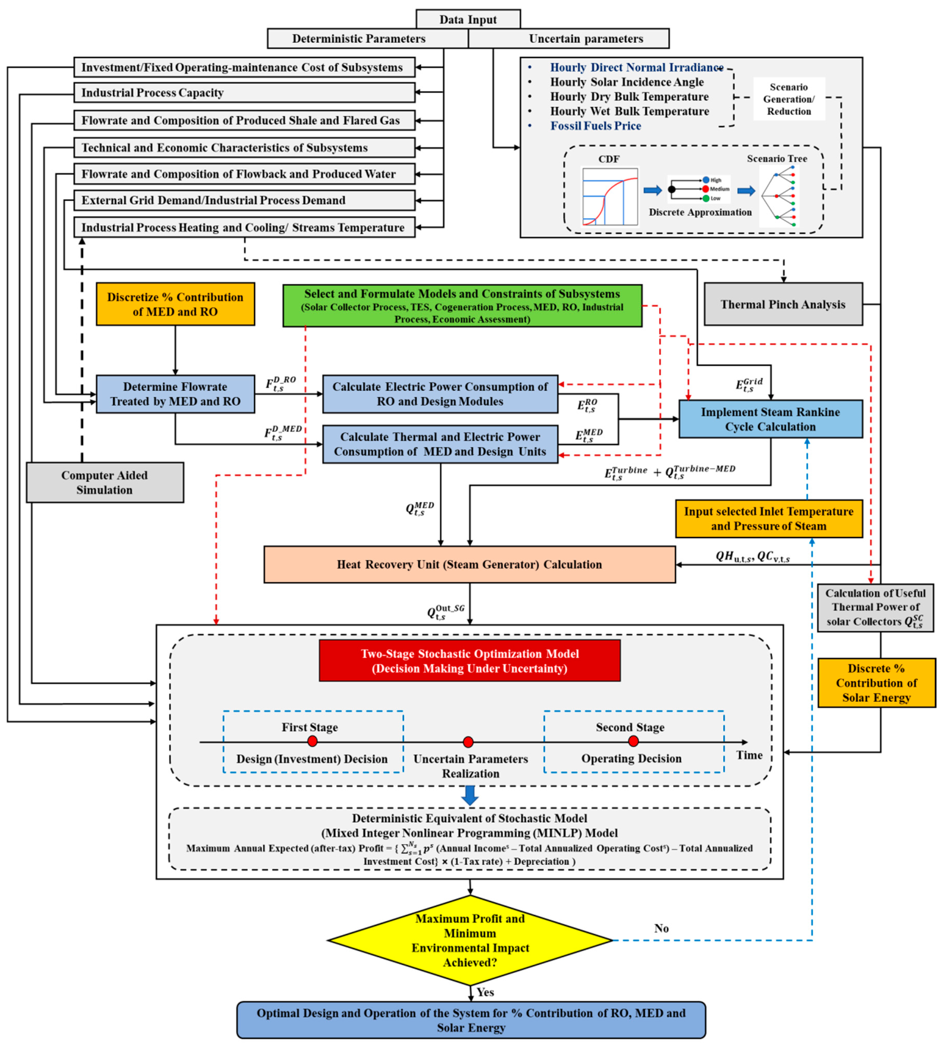
3. Approach

The proposed approach is designed to identify the optimal configuration, design, and operation of the integrated system while aiming to maximize the annual profit under uncertainty. The first step is to construct a superstructure that embeds meaningful configuration and system integration opportunities. Figure 1 is a schematic representation of the proposed superstructure. Each component in the superstructure is modeled (both steady-state and dynamic operations).

The complexity of integrating the various subsystems, handling multiple scales, and addressing the diurnal and uncertain nature of solar energy pose a major challenge, which requires the development of a methodical approach. Figure 2 demonstrates the structure of the proposed hierarchical approach. The starting step in the proposed approach is to obtain deterministic and uncertain data. The scenario-based method is adopted to describe the uncertain parameters during all the time periods with an identified probability of occurrence based on a discrete approximation of continuous distributions, which allows reformulating a stochastic programming problem as a deterministic equivalent of a stochastic programming model with a finite number of scenarios to describe the uncertainty, for more detailed information is given in Section 3.1. Next, the percentage contribution of RO and MED in treating wastewater is iteratively discretized, which leads to simplifying the solving of the optimization problem and raising computational efficiency. The RO and MED plants can be designed separately based on their known treatment tasks for each discretization step. Hence, thermal and power loads for plants are calculated. Similar approaches have been proposed earlier in the literature for other applications [13,39]. Furthermore, various percentage of solar energy contribution in the total mix of thermal power that supplied to the system is chosen to add further simplifying to a computational approach and to assess the economic feasibility of incorporating solar energy to the system. Computer-aided simulation is used to estimate the heat duties of major equipment and streams temperature for an industrial process. Heat integration approach can be used to determine the deficit and surplus heat of an industrial process that can be coupled with the heat recovery unit (steam generator) of the system. Therefore, thermal pinch analysis technique [40] is used to integrate the hot and cold streams of an industrial process to calculate deficit and excess heat and the temperature at which it is available. Another important step is to select and formulate a set of models and constraints that characterize the subsystems involved in the entire system as in Section 3.3. Once the foregoing steps are achieved and the total thermal and electric loads are determined of the integrated system, the optimization problem is formulated as a multi-scenario mixed integer non-linear programming (MINLP) problem that is a deterministic equivalent of a two-stage stochastic programming model with recourse to dealing with an uncertainty of solar energy and fossil fuels price for each period, more detailed information in Section 3.2 and Section 3.4. The objective function is solved to minimize the sum of the capital costs (First stage), which are expended only once at the time of building the system and the operating costs (Second stage), which are expended during each scenario along with maximizing the system revenue. Upon identification of the total annual profit and the thermal power mix of the system by reconciling of economic and environmental objectives, the procedure is repeated for the various percentage contribution of RO and MED in treating wastewater. The obtained results are compared to select the maximum-profit solution and the optimal design and operation of the entire system.

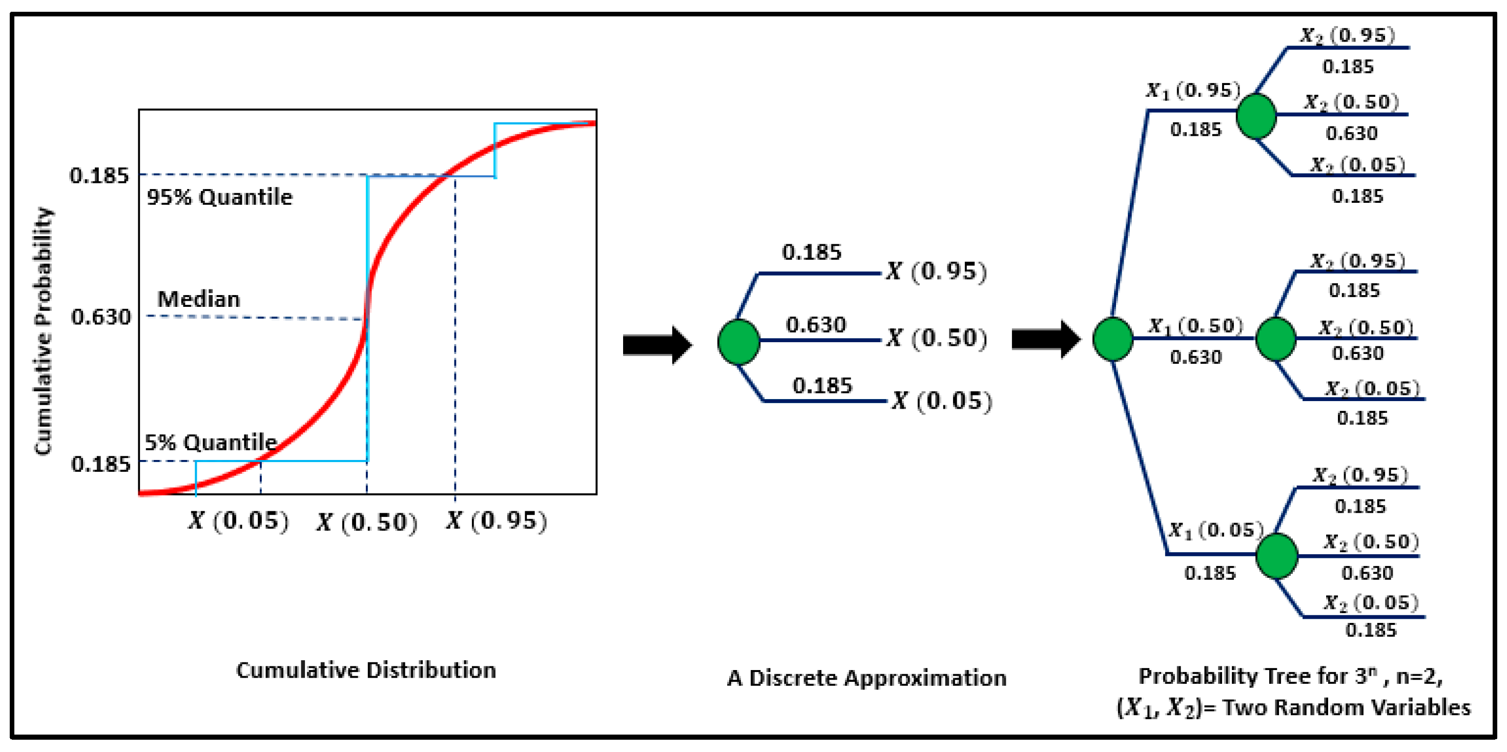
3.1. Generating Scenario Tree for Uncertain Parameters

The precise dealing with the required input data is very significant in enhancing the computational efficiency of solving optimization problems. The input data are classified into deterministic and uncertain parameters. Deterministic input parameters are utilized in the model, specifically, the decision of selecting and designing the system units before the realization of uncertain parameters such as capital cost investment, fixed operation and maintenance cost, techno-economic characteristics, etc. Otherwise, it is generally intractable to optimize a stochastic problem by incorporating uncertain parameters as continuous random variables. Thus, these parameters can be represented as a multi-period scenario tree, which grows with scenario tree nodes based on approximating continuous distributions into discrete distributions or Monte Carlo simulation random generated nodes (a random generation of information) from the common continuous distributions [41]. A scenario tree is represented by a set of nodes,$\mathrm{k}\mathsf{ϵ}\mathrm{K}$, and branches. Each scenario $\mathrm{s}$ is a path of flowing all possible information and realizing uncertain parameters. This path starts from the initial situation (which is called the root node) to a leaf node through the time horizon of a stochastic problem and it has a certain probability, ${\mathrm{p}}^{\mathrm{s}}={\mathsf{П}}_{\mathrm{k}\mathsf{ϵ}\mathrm{K}}{\mathrm{p}}_{\mathrm{k}}^{\mathrm{s}}$, which is the product of the occurrence probability (joint probability) of all nodes pertaining to the path. It is necessary to mention that the sum of the probability of all scenarios within a certain period in the time horizon is to be equal to one ${\mathsf{\Sigma }}_{\mathrm{s}}{\mathrm{P}}_{\mathrm{t}}^{\mathrm{s}}=1$. The main goal of scenario generation in the stochastic problem is to create a set of probabilistic scenarios, which describe precisely uncertain parameters space to make the best decisions for the first and second stages of a two-stage stochastic model.

In this work, the integrated system was subjected to significant uncertainties in solar-irradiation intensity (direct normal irradiance) and fossil fuels (natural gas) price, which take on finite values at different points of time, particularly, from season to another season of a year, during system operation. Note that the natural gas demand peaks in the winter are higher than demand peaks in the summer due to the higher gas consumption in heating and power generation. The seasonal fluctuation of demand leads to significant price change. To illustrate, the U.S. gas market has two seasons: The surplus gas is stored by injecting into the ground in summer (April–October), while it is withdrawn in winter (November–March) to meet the increased demand [42]. Consequently, the exploiting of solar energy as an energy source could contribute in increasing gas amount stored in summer due to the high intensity of solar irradiation, but this contribution is less important in winter because fluctuations in hourly direct normal irradiance are weak in summer but strong in winter. Accordingly, the uncertainty of solar energy and fossil fuels price can be represented by three scenario tree nodes (high, medium, and low) with their appointed probabilities based on discrete approximations of continuous distributions to generate a finite number of ${\mathrm{N}}_{\mathrm{s}}$ probabilistic scenarios included in a set S = $\left\{\mathrm{s}|\mathrm{s}=1,\dots ,{\mathrm{N}}_{\mathrm{s}}\right\}.$ The use of a finite number of scenarios for uncertain parameters can lead to reducing the complexity of a stochastic problem and computational costs by reformulating the two-stochastic stage model as a deterministic-equivalent model. In this work, the three-point Pearson–Tukey approximation technique for continuous probability distributions (e.g., normal, uniform, and exponential) was used to substitute the entire continuous probability distribution by a few representative values (N discrete points) and their identified probabilities, which weights the 0.05, 0.50, and 0.95 percentiles by 0.185, 0.630, and 0.185 respectively, as shown in Figure 3. The three-point Pearson–Tukey (3-PT) approximation shows a great accuracy comparing with Monte Carlo simulation, comparisons have been made for the mean of a random variable and for conventional functions of one and two variables using a assort of known distributions. The using 3-PT would facilitate a problem solution because it requires the evaluation of only 3ⁿ scenarios, where n is the number of random variables in the model. This technique that can match the first (2N−1) statistical moments statistical features (mean, variance, max, kurtosis, and skewness) of the continuous distribution, where N is the number of discrete points [43,44,45,46,47,48]. The first task for modeling the operating system mathematically under uncertainty is to represent uncertain parameters using probabilistic scenarios, which is defined as scenario generation.

In addition to using the number of uncertain parameters, as abovementioned, in estimating the number of scenarios, the number of stages or time periods proposed in the optimization problem were also used for the same purpose. Consequently, the number of scenarios could be calculated by the relationship $3^{\mathrm{n}.\mathrm{t}}$ or $3^{\mathrm{n}.\left(\mathrm{T}-1\right)}$, where n is the number of uncertain parameters in the model, t is the number of a specific period time, and T is the number of stages. It is worth noting that the length of each time stage can be planned according to modeling requirements (can be a period or multiple period time). In this work, a time horizon of the system operating represented one year, which could be divided into two or four time periods depending on the geographical site that determines a season length and the number of months associated with each season. To illustrate, if two uncertain parameters described by three nodes (high, medium, and low) and four multiple periods represented by four seasons (e.g., spring, summer, fall, and winter) were considered, Hence, at the end of the fourth period, $3^8$ scenarios were generated. Similar approaches have been adopted in the literature of other applications [29,41,49]. The next step was to keep fewer scenarios possible to ensure that the problem of stochastic optimization could be solved with a reasonable computational effort. The scenario tree may grow exponentially with a significant increase in the number of time periods or stages. In such cases, several scenario reduction techniques such as forward selection, backward reduction, and K-means clustering algorithm can be adopted to decrease the scenario numbers that leads to minimize the computational time and cost of the optimization problems to be computationally tractable, these techniques used in various applications can be found in the literature [49,50,51,52,53]. In the same context, some researchers observed that the results with suitable accuracy can be obtained, when the number of scenarios is reduced to one quarter and the computational time is lowered four times [50]. Other investigators have the opposite opinion regarding the scenario reduction and it may cause a high error rate of an objective function value and jeopardize the accuracy of the modeling [54]. To reduce the number of scenarios, the model size, and computational requirements of this work, the three-point approximation technique is used to represent the uncertain parameters by a finite set of known values, in addition, to select typical seasons (time periods) that represent the full yearly horizon.

3.2. Two-Stage Stochastic Optimization Model

The optimal configuration of an integrated system requires considering all the design alternatives through the interconnection between system units operating under uncertain operating conditions. These uncertainties subject to several technical and commercial parameters, which may not be fully revealed at the early stages of the system design. It is obvious that the incorporation of uncertain aspects in the optimization problems causes the transformation of a deterministic problem (which can be solved by using standard methods of mathematical programming) to a stochastic problem (which requires special techniques and approaches to be solved). The incorporation of uncertain parameters makes the deterministic model is unsuitable to optimize the expected value of net profit in this work. A generally mathematical representation of the final structure and design under uncertainty can be presented as in the following form [55]:

$$\mathrm{P}=\underset{\mathrm{y},\mathrm{d},\mathrm{z}}{\max }\mathrm{f}\left(\mathrm{y},\mathrm{d},\mathrm{z},\mathrm{x},\mathsf{\theta }\right),$$

(1)

$$\begin{gathered} \mathrm{s}.\mathrm{t}. \\ \mathrm{h}\left(\mathrm{y},\mathrm{d},\mathrm{z},\mathrm{x},\mathsf{\theta }\right)=0, \\ \mathrm{g}\left(\mathrm{y},\mathrm{d},\mathrm{z},\mathrm{x},\mathsf{\theta }\right)\le 0, \\ \mathrm{d}\mathsf{ϵ}\mathrm{D},\mathrm{z}\mathsf{ϵ}\mathrm{Z},\mathrm{x}\mathsf{ϵ}\mathrm{X},\mathrm{y}\mathsf{ϵ}{\left\{0,1\right\}}^{\mathrm{m}}, \\ \mathsf{\theta }\mathsf{ϵ}{\mathcal{R}}^{\mathrm{n}}, \end{gathered}$$

where $\mathrm{P}$ is the profit, $\mathrm{f}$ is a scalar objective function (an economic performance index), which must be optimized to find the maximum or minimum value, $\mathrm{y}$ is the vector of binary 0–1 variables for existing units, $\mathrm{d}$ is the vector of design variables (e.g., physical size of installed units), $\mathrm{z}$ and $\mathrm{x}$ represent the vectors of control and state variables (operating conditions), and $\mathsf{\theta }$ is the vector of uncertain parameters. The set of equality constraints ($\mathrm{h}$) are process equations (energy and mass balances), while the set of inequalities ($\mathrm{g}$) be compatible with the design specifications and logical constraints, which also represents the linking constraints (hard constraints) that use to unify the choices of design decisions of the first-stage across all operational periods of the second-stage scenarios, otherwise, these constraints link the design variables with the variables of each scenario [56,57].

A two-stochastic programming model with recourse is the most commonly used technique to deal with decision making under uncertainty in mathematical programming. Particularly, when this technique is used for solving problems of a large superstructure of an integrated system or extensive portion of a process plant by breaking these problems down into smaller independent components because each operational scenario may represent a large-scale optimization problem. In the same context, the mathematical programming problem accommodates very large decisions in the first stage and any number of subproblems in the second stage [57]. A general formulation of this model can be found in [50], which can be used to maximize or minimize the expected value of an objective function for all scenarios considered under an uncertain future. The general formula of Equation (1) can be formulated in the two-stage stochastic programming framework. Consequently, the two-stage stochastic programming model is adopted to formulate the superstructure of the system. Hence, the superstructure variables can be classified as either design or operational variables. In the first stage, the essential units of the system with the design variables of each unit (e.g., solar collection area, thermal storage volume, evaporator area of MED, membrane area of RO, etc.) should be chosen, but the selected units may not be necessarily compatible with operational conditions of all possible time periods or scenarios. Once the design variables are decided, the operational aspects can be optimized over the time horizon for all scenarios according to the decisions made in the first stage. Therefore, a duplicate method is substantial to discretize the horizon time period iteratively in which the design variables are replaced along with adjusting the operating conditions until obtaining an optimal design, which is feasible over a certain range of operating conditions, by minimizing expected (investment and operating) costs and maximizing expected (profit) through the two stages.

It is worth noting that it is not necessary to be the consistent relationship between stages and time periods. Therefore, in specific cases, all-time periods can be lumped into the second stage of a stochastic programming model [58]. Therefore, it can be assumed that all time periods are accommodated in the second stage for the problem of this work, as shown in Figure 4. To avoid the challenges and complexity in modeling and find the optimal solution for the system, a finite number of scenarios can be postulated to describe the randomness by representing finite values of the uncertain parameters in multiple scenarios. Hence, the operational pattern of the system can be adjusted for each scenario over all periods in the time horizon with maintaining the same system configuration and fixed capacity of the subsystems that determined in the first stage. Based on that, the objective function of the total expected profit, which accommodates the cost of the selected design and the expected optimal profit (revenue of sales and operating costs), can be optimized by allowing the transformation of the two-stage stochastic programming model into a multi-scenario mixed integer non-linear programming (MINLP) model that is a deterministic equivalent model as follows [55]:

$$\mathrm{P}=\underset{\mathrm{y},\mathrm{d}}{\max }\{{\mathrm{E}}_{\mathsf{\theta }}\{{\mathrm{f}}_{\mathrm{s}}\left(\mathrm{y},\mathrm{d},{\mathsf{\theta }}_{\mathrm{s}}\right)\}-{\mathrm{f}}^0\left(\mathrm{d}\right)-\mathrm{cy},$$

(2)

$\mathrm{where}$:

$$\begin{gathered} {\mathrm{f}}_{\mathrm{s}}\left(\mathrm{y},\mathrm{d},{\mathsf{\theta }}_{\mathrm{s}}\right)=\underset{{\mathrm{z}}_{\mathrm{s}}}{\max }{{\displaystyle \sum }}_{\mathrm{s}=1}^{{\mathrm{N}}_{\mathrm{s}}}{\mathrm{p}}_{\mathrm{s}}{\mathrm{f}}_{\mathrm{s}}\left(\mathrm{y},\mathrm{d},{\mathrm{z}}_{\mathrm{s}},{\mathrm{x}}_{\mathrm{s}},{\mathsf{\theta }}_{\mathrm{s}}\right), \\ \mathrm{s}.\mathrm{t}. \\ {\mathrm{h}}_{\mathrm{s}}\left(\mathrm{y},\mathrm{d},{\mathrm{z}}_{\mathrm{s}},{\mathrm{x}}_{\mathrm{s}},{\mathsf{\theta }}_{\mathrm{s}}\right)=0, \\ {\mathrm{g}}_{\mathrm{s}}\left(\mathrm{y},\mathrm{d},{\mathrm{z}}_{\mathrm{s}},{\mathrm{x}}_{\mathrm{s}},{\mathsf{\theta }}_{\mathrm{s}}\right)\le 0, \\ \mathrm{d}\mathsf{ϵ}\mathrm{D},{\mathrm{z}}_{\mathrm{s}}\mathsf{ϵ}\mathrm{Z},{\mathrm{x}}_{\mathrm{s}}\mathsf{ϵ}\mathrm{X},\mathrm{y}\mathsf{ϵ}{\left\{0,1\right\}}^{\mathrm{m}}, \\ {\mathsf{\theta }}_{\mathrm{s}}\mathsf{ϵ}\mathrm{J}\left({\mathsf{\theta }}_{\mathrm{s}}\right), \\ \mathsf{\theta }\mathsf{ϵ} \mathcal{R}\left(\mathrm{d}\right), \end{gathered}$$

where $\mathrm{P}$ is the total expected profit of the system, ${\mathrm{f}}_{\mathrm{s}}$ is a profit function, which represents the total expected revenue and operating cost of the system for all the scenarios, ${\mathrm{f}}^0\left(\mathrm{d}\right)$ is the capital cost function of the design, $\mathrm{cy}$ represents a fixed charge cost, ${\mathrm{E}}_{\mathsf{\theta }}$ is the expectancy operator, ${\mathrm{p}}_{\mathrm{s}}$ represents the probability assigned to the occurrence of the ${\mathrm{N}}_{\mathrm{s}}$ scenarios, and $\mathrm{J}\left({\mathsf{\theta }}_{\mathrm{s}}\right)$ is a probabilistic density function.

Prior to uncertainty realization, the first stage decisions (here and now) could be implemented immediately on the design aspects (i.e., selection and capacity of the subsystems) of the integrated system to specify an optimal vector of the design variables $\mathrm{d}$ while seeking for determining an optimal vector of control variables $\mathrm{z}$ (operational flexibility and feasibility) in the second stage (wait and see) for every uncertain realization θ, which are lying with the associated feasible region $\mathcal{R}$. Note that $\mathcal{R}$ represents the feasible region of the design $\mathrm{d}$, $\mathsf{\theta }\mathsf{ϵ} \mathcal{R}\left(\mathsf{\theta }\right)$, and $\mathrm{R}\left(\mathrm{d}\right)=\left\{\mathsf{\theta }|\forall \mathsf{\theta }\mathsf{ϵ}\mathrm{R}\mathsf{Ǝ}\mathrm{z}:\mathrm{f}\left(\mathrm{d},\mathrm{z},\mathsf{\theta }\right)\le 0\right\}$ [37]. The problem of feasibility can be addressed by considering further penalty functions or through transforming to the deterministic equivalent multiperiod problem by postulating a finite number of discrete points of uncertain parameters $\mathsf{\theta }$ [59], as mentioned in Section 3.1. Once the first decisions are made to estimate the capital cost of the design, the design variables cannot be changed over the time horizon of the second stage when the system is being operated. While the second stage decisions could be delayed until the appearance of uncertainty to carry out it on the operating pattern to evaluate the operating cost expenditure, which is highly dependent on the selecting of design variables of the first stage. It should be noted that the operational variables are scenario dependent to consider uncertain parameters, which are significant in taking recourse action in the second stage.

3.3. Modeling Formulation

The formulation and selecting of suitable models are considered the significant steps to properly describe the main building blocks of the system, which was presented in Figure 1. The detailed equations are used for the models as follows:

3.3.1. Solar Collection Process

A parabolic trough collector was selected to represent the solar collection process, which is incorporated in the system as the direct or indirect source of thermal power for the entire system. The modeling of the solar collection process was developed basing on literature models and data [13,60,61,62,63], as described in

Table A1. General modeling equations for solar collection process.

Equation		Description
${\mathrm{Q}}_{\mathrm{sun}\to \mathrm{collector}}$ = $\mathrm{DNI}.\cos \mathsf{\theta }.{\mathrm{W}}_{\mathrm{c}}$	(52)	Thermal power (W/m), which can be produced by the solar collection process when the direct normal irradiance (DNI) hits the collector aperture	[61]
$\cos \mathsf{\theta }=\sqrt{{\cos }^2{\mathsf{\theta }}_{\mathrm{z}}+{\cos }^2\mathsf{\delta }.{\sin }^2\mathsf{\omega }}$	(53)	Incidence angle for the north–south orientation	[61]
${\mathrm{Q}}_{\mathrm{collector}\to \mathrm{reciever}}=\mathrm{DNI}.\cos \mathsf{\theta }.{\mathrm{W}}_{\mathrm{c}}.{\mathsf{\eta }}_{\mathrm{opt}}.\mathrm{K}\left(\mathsf{\theta }\right).{\mathrm{F}}_{\mathrm{f}}.{\mathrm{R}}_{\mathrm{SL}}.{\mathrm{O}}_{\mathrm{EL}}$	(54)	Thermal power (W/m), which can be absorbed by a receiver tube of a collection system loop	[13]
${\mathsf{\eta }}_{\mathrm{opt}}=\mathsf{\rho }.\mathsf{\gamma }.\mathsf{\tau }.\mathsf{\alpha }$	(55)	Peak optical efficiency of a collector when the incidence angle on the aperture plane is 0o	[60]
$\mathrm{K}\left(\mathsf{\theta }\right)=1-2.23073\times {10}^{-4}.\mathsf{\theta }-1.1\times {10}^{-4}$.${\mathsf{\theta }}^2+3.18596\times {10}^{-6}.{\mathsf{\theta }}^3-4.85509\times {10}^{-8}.{\mathsf{\theta }}^4,$$0^0\le \mathsf{\theta }\le {80}^0$$\mathrm{K}\left(\mathsf{\theta }\right)$ = 0 $\mathsf{\theta }>{80}^{\mathrm{o}}$	(56)	Incidence angle modifier for a LS-3 collector	[60]
${\mathrm{R}}_{\mathrm{SL}}=\min \left[\max \left(0.0,\frac{{\mathrm{L}}_{\mathrm{spacing}}}{{\mathrm{W}}_{\mathrm{c}}}.\frac{\cos {\mathsf{\theta }}_{\mathrm{z}}}{\cos \mathsf{\theta }}\right);1.0\right]$	(57)	Row shadow factor	[62]
${\mathrm{O}}_{\mathrm{EL}}=1-\frac{\mathrm{f}.\tan \mathsf{\theta }}{{\mathrm{L}}_{\mathrm{SCA}}}$	(58)	Optical end loss	[62]
${\mathrm{Q}}_{\mathrm{collector}\to \mathrm{ambient}}={\mathrm{U}}_{\mathrm{rec}}.\mathsf{\pi }.{\mathrm{d}}_{\mathrm{o}}$.(${\mathrm{T}}_{\mathrm{rec}}-{\mathrm{T}}_{\mathrm{amb}})$	(59)	Total thermal power (W/m), which may be lost from a collector represents the combination of the radiative heat loss from the receiver pipe to the ambient environment ${\mathrm{Q}}_{\mathrm{reciever}\to \mathrm{ambient}}$ and convective and conductive heat losses from the receiver pipe to its outer glass pipe ${\mathrm{Q}}_{\mathrm{receiver}\to \mathrm{glass}}$	[60]
${\mathrm{U}}_{\mathrm{rec}}=\mathrm{a}+\mathrm{b}\left({\mathrm{T}}_{\mathrm{rec}}-{\mathrm{T}}_{\mathrm{amb}}\right)+\mathrm{c}{({\mathrm{T}}_{\mathrm{rec}}-{\mathrm{T}}_{\mathrm{amb}})}^2$	(60)	Overall heat transfer coefficient of a collector is found experimentally depending on a receiver pipe temperature	[60]
${\mathrm{Q}}_{\mathrm{collector}\to \mathrm{fluid}}={\mathrm{Q}}_{\mathrm{collector}\to \mathrm{receiver}}-{\mathrm{Q}}_{\mathrm{collector}\to \mathrm{ambient}}$	(61)	Thermal power (W/m), which can be transferred from a collector to a fluid	[13]
${\mathrm{Q}}_{\mathrm{LFP}}=0.0583.{\mathrm{W}}_{\mathrm{c}}.\left({\mathrm{T}}_{\mathrm{rec}}-{\mathrm{T}}_{\mathrm{amb}}\right)$	(62)	Thermal power (W/m), which may be lost from the headers (pipes)	[61]
${\mathrm{Q}}_{\mathrm{LFV}}=0.0497.{\mathrm{W}}_{\mathrm{c}}.\left({\mathrm{T}}_{\mathrm{rec}}-{\mathrm{T}}_{\mathrm{amb}}\right)$	(63)	Thermal power (W/m), which may be lost from the expansion tank (vessel)	[61]
${\mathrm{Q}}_{\mathrm{PTC}\to \mathrm{final}\mathrm{demand}}={\mathrm{Q}}_{\mathrm{collector}\to \mathrm{receiver}}-{\mathrm{Q}}_{\mathrm{collector}\to \mathrm{ambient}}-{\mathrm{Q}}_{\mathrm{LFP}}-{\mathrm{Q}}_{\mathrm{LFV}}$	(64)	Net useful thermal power (W/m), which can be produced by the solar collection process	[13]

.

3.3.2. Thermal Energy Storage

Thermal storage is utilized to assist in supplying a steady thermal power to the system by manipulating the dynamic variability of solar energy. An indirect thermal storage system is selected that consists of two separated tanks. A binary molten salt (sodium and potassium nitrate) is used as the storage media. To describe the performance of the thermal storage system, the required equations are described in

Table A2. General modeling equations for thermal energy storage.

Equation		Description
${\mathrm{Q}}_{\mathrm{in}}={\mathrm{m}}_{\mathrm{ms}}.{\mathrm{C}}_{\mathrm{Pms}}.\left({\mathrm{T}}_{\mathrm{HT}}-{\mathrm{T}}_{\mathrm{CT}}\right)={\mathsf{\eta }}_{\mathrm{EX}}.{\mathrm{m}}_{\mathrm{oil}}.{\mathrm{C}}_{\mathrm{P},\mathrm{oil}}.\left(\mathsf{\Delta }\mathrm{T}\right)$	(65)	Inlet thermal power (W) of the thermal storage (charge process)	[13]
${\mathrm{Q}}_{\mathrm{out}}={\mathrm{m}}_{\mathrm{oil}}.{\mathrm{C}}_{\mathrm{Poil}}.\left(\mathsf{\Delta }\mathrm{T}\right)={\mathsf{\eta }}_{\mathrm{EX}}.{\mathrm{m}}_{\mathrm{ms}}.{\mathrm{C}}_{\mathrm{Pms}}.\left({\mathrm{T}}_{\mathrm{HT}}-{\mathrm{T}}_{\mathrm{CT}}\right)$	(66)	Outlet thermal power (W) of the thermal storage (discharge process)	[13]
${\mathrm{C}}_{\mathrm{Pms}}$ = $1443+0.172{\mathrm{T}}_{\mathrm{ms}}$	(67)	Specific heat of the molten salt	[93]
${\mathrm{Q}}_{\mathrm{TES}}={\mathrm{Q}}_{\mathrm{acc}}+{\mathrm{Q}}_{\mathrm{in}}-{\mathrm{Q}}_{\mathrm{out}}-{\mathrm{Q}}_{\mathrm{loss}}$	(68)	Net thermal power (W) inside the tank	[13]
${\mathrm{Q}}_{\mathrm{loss}}=0.00017.{\mathrm{T}}_{\mathrm{ms}}+0.012$	(69)	thermal power loss (kW/m2) of the cold and heat tanks	[93]

.

3.3.3. Cogeneration Process

The co-production of power and low-grade steam for the entire system can be achieved by the cogeneration process, which is based on a Rankine cycle. This process consists of a boiler (or a steam generator that used in this work to utilize various energy sources), a steam turbine, and a condenser, which is replaced with a multiple-effect distillation plant to exploit the surplus heat production. The modeling of the Rankine cycle requires appropriate correlations for the thermodynamic properties to use in the optimization formulations. The complicated nature of available correlations of steam tables (e.g., nonlinear, and nonconvex function) and the complexity of incorporating these correlations into an optimization task to find the optimal values of a Rankine cycle were significant motivation to develop a new set of thermodynamic correlations that could be inserted easily into the optimization formulation for a cogeneration design. In this study, a set of correlations, which has been developed in the literature [21], was adopted to estimate the properties of steam. These correlations and fundamental equations are shown in

Table A3. General modeling correlations and equations of steam Rankine cycle (SRC).

Equation		Description
${\mathrm{T}}_{\mathrm{sat}}=112.72.{\mathrm{P}}_{\mathrm{sat}}^{0.2289}$	(70)	Saturated temperature as a function of pressure (can be used at the outlet of a condenser or at the inlet of a boiler), Error = ±0.64%	[21]
${\mathrm{h}}_{\mathrm{sat}}^{\mathrm{f}}=0.2674.{\mathrm{T}}_{\mathrm{sat}}^{1.2127}$	(71)	Saturated liquid enthalpy (can be used at the outlet of a condenser or at the inlet of a boiler),$\mathrm{P}\le 2500\mathrm{psi},$ Error = ±3%	[21]
${\mathrm{s}}^{\mathrm{v}}=\left(-0.5549.\ln \left({\mathrm{T}}_{\mathrm{sat}}\right)+3.7876\right).{\mathrm{T}}^{0.1001.\exp \left(0.0017.{\mathrm{T}}_{\mathrm{sat}}\right)}$	(72)	Entropy of steam (can be used at the inlet of a turbine), $\mathrm{P}\le 2500\mathrm{psi},$ $\mathrm{T}\le 1500°\mathrm{F},$ Error = ±3.5%	[21]
${\mathrm{h}}^{\mathrm{v}}=0.2029.{\mathrm{T}}_{\mathrm{sat}}.{({\mathrm{s}}^{\mathrm{v}})}^{3.647}+817.35$	(73)	Enthalpy of steam (can be used at the inlet of a turbine or at the outlet of a turbine),$14.7\le \mathrm{P}\le 2000\mathrm{psi},$ Error = ±0.6%	[21]
$\Delta {\mathrm{h}}_{\mathrm{is}}={\mathrm{h}}^{\mathrm{v}}-{\mathrm{h}}_{\mathrm{is}}^{\mathrm{v}}$	(74)	Isentropic enthalpy difference	[21]
${\mathrm{h}}_{\mathrm{act}}^{\mathrm{v}}={\mathrm{h}}^{\mathrm{v}}-{\mathsf{\eta }}_{\mathrm{is}}.\Delta {\mathrm{h}}_{\mathrm{is}}$	(75)	Actual enthalpy at the outlet of a turbine	[21]
$\mathrm{m}=\frac{{\mathrm{Q}}_{\mathrm{process}}}{{\mathrm{h}}_{\mathrm{act}}^{\mathrm{v}}-{\mathrm{h}}_{\mathrm{sat}}^{\mathrm{f}}}$	(76)	Mass flow rate in term of the required heat of the process (condenser)	[21]
$\mathrm{T}=\frac{{\mathrm{h}}_{\mathrm{act}}^{\mathrm{v}}-\mathrm{B}\left(\mathrm{s}\right)}{\mathrm{A}\left(\mathrm{s}\right)}$	(77)	Outlet temperature of a turbine	[21]
$\mathrm{A}\left(\mathrm{s}\right)=-0.7918.{({\mathrm{s}}^{\mathrm{v}})}^3+3.4575.{({\mathrm{s}}^{\mathrm{v}})}^2+4.5513.{\mathrm{s}}^{\mathrm{v}}+2.1267$
$\mathrm{B}\left(\mathrm{s}\right)=710.22.{({\mathrm{s}}^{\mathrm{v}})}^3+3910.6.{({\mathrm{s}}^{\mathrm{v}})}^2+7117.3.{\mathrm{s}}^{\mathrm{v}}-3253.5$
${\mathrm{Q}}_{\mathrm{Boiler}}=\mathrm{m}\left({\mathrm{h}}^{\mathrm{v}}-{\mathrm{h}}_{\mathrm{sat}}^{\mathrm{f}}\right)$	(78)	Thermal power output of a boiler	[21]
${\mathrm{Q}}_{\mathrm{Boiler}}={\mathrm{Q}}_{\mathrm{Fuel}}.{\mathsf{\eta }}_{\mathrm{Fuel}}$
${\mathrm{m}}_{\mathrm{F}}=\frac{{\mathrm{Q}}_{\mathrm{Boiler}}}{{\mathrm{H}}_{\mathrm{v},\mathrm{F}}.{\mathsf{\eta }}_{\mathrm{boiler}}}$	(79)	Mass flow rate of fuel is provided to a boiler	[21]
${\mathrm{E}}_{\mathrm{Turbine}}=\mathrm{m}\left({\mathrm{h}}^{\mathrm{v}}-{\mathrm{h}}_{\mathrm{act}}^{\mathrm{v}}\right)$	(80)	Turbine shaft power output	[21]

.

While the turbine hardware model, which was developed in the literature [22], can be used to obtain the isentropic efficiency for the steam turbine. The hardware model shows the variation of efficiency with operating conditions, a load, and a turbine size, as in

Table A4. Turbine hardware model.

Equation		Description
${\mathsf{\eta }}_{\mathrm{is}}=\frac{6}{5\mathrm{B}}\left(1-\frac{3.41443\times {10}^6\times \mathrm{A}}{\Delta {\mathrm{h}}_{\mathrm{is}}\times {\mathrm{m}}^{\max }}\right)\left(1-\frac{{\mathrm{m}}^{\max }}{6\times \mathrm{m}}\right)$	(81)	Isentropic efficiency for a turbine ${\mathrm{a}}_{\mathrm{o}}$, ${\mathrm{a}}_1$, ${\mathrm{a}}_2$, and ${\mathrm{a}}_3$ are turbine regression coefficient [73]	[22]
$\mathrm{A}={\mathrm{a}}_{\mathrm{o}}+{\mathrm{a}}_1.{\mathrm{T}}_{\mathrm{sat}}$
$\mathrm{B}={\mathrm{a}}_2+{\mathrm{a}}_3.{\mathrm{T}}_{\mathrm{sat}}$
${\mathsf{\eta }}_{\mathrm{is}}=\frac{1}{\mathrm{B}}\left(1-\frac{3.41443\times {10}^6\times \mathrm{A}}{\Delta {\mathrm{h}}_{\mathrm{is}}\times {\mathrm{m}}^{\max }}\right)$	(82)	Isentropic efficiency for a turbine when m = ${\mathrm{m}}^{\max }$ at design condition	[22]

.

3.3.4. Desalination Process

To make the proposed system contributes effectively in managing water resources on-site, the hybrid combination of two desalination plants (included MED and RO) has been considered to supply the freshwater to the entire system by recycling/reusing the wastewater. Indeed, the multiple-effect distillation (MED) plant is used to improve the efficiency of the system by exploiting the surplus low-grade heat of the cogeneration process and an industrial process, while the reverse osmosis (RO) plant is used to add a significant feature to the system (to be more flexible) by covering the largest area of treated water demand due to the ability of installing the RO plant in another geographical location. The performance modeling of desalination plants has been described through detailed equations of energy and mass balance. The average condition (AC) model, which is the simplified version of the shortcut method for the modeling MED plant (based on forward-feed MED systems without flashing effects), has been taken from [40]. The main equations of the AC model are given in

Table A5. General modeling equations and correlations of the MED plant.

Equation		Description
${\mathrm{Q}}_{\mathrm{Total}}={\mathrm{Q}}_{\mathrm{htffe}}.\mathrm{N}$	(83)	Total thermal power loads (W) of all evaporators (assumed an equal thermal load of all evaporators)	[40]
${\mathrm{Q}}_{\mathrm{Total}}=\Delta {\mathrm{H}}_{\mathrm{c},\mathrm{avg}}.{\mathrm{m}}_{\mathrm{D}}$
$\Delta {\mathrm{H}}_{\mathrm{c},\mathrm{avg}}=2.7532.{\mathrm{T}}_{\mathrm{vapor},\mathrm{avg}}+3278.8$	(84)	Latent heat of condensation	[40]
${\mathrm{T}}_{\mathrm{vapor},\mathrm{avg}}=\frac{{\mathrm{T}}_{\mathrm{vapor},0}+{\mathrm{T}}_{\mathrm{vapor},\mathrm{N}}}{2}$	(85)	Average temperature of the vapor	[40]
${\mathrm{Q}}_{\mathrm{htffe}}={\mathrm{U}}_{\mathrm{httfe}}.{\mathrm{A}}_{\mathrm{httfe}}.\Delta {\mathrm{T}}_{\mathrm{vapor}}$	(86)	Thermal power (W) emitted by condensing distilled water into the tubes of the horizontal-tube falling film evaporator (HTFFE)	[40]
${\mathrm{U}}_{\mathrm{htffe}}=0.8552+4.7\times {10}^{-3}\times {\mathrm{T}}_{\mathrm{vapor},\mathrm{avg}}$	(87)	Overall heat transfer coefficient	[40]
$\Delta {\mathrm{T}}_{\mathrm{vapor},\mathrm{avg}}=\frac{{\mathrm{T}}_{\mathrm{vapor},0}-{\mathrm{T}}_{\mathrm{vapor},\mathrm{N}}}{\mathrm{N}}$	(88)	An average temperature driving force of evaporators by assuming an equal vapor temperature drop for each MED evaporator	[40]
${\mathrm{m}}_{\mathrm{F}}={\mathrm{m}}_{\mathrm{D}}+{\mathrm{m}}_{\mathrm{B}}$	(89)	Overall balance for the MED plant	[40]
${\mathrm{m}}_{\mathrm{F}}.{\mathrm{x}}_{\mathrm{F}}={\mathrm{m}}_{\mathrm{D}}.{\mathrm{x}}_{\mathrm{D}}+{\mathrm{m}}_{\mathrm{B}}.{\mathrm{x}}_{\mathrm{B}}$	(90)	Overall salt balance for the MED plant	[40]
$\frac{{\mathrm{m}}_{\mathrm{D}}}{{\mathrm{m}}_{\mathrm{F}}}=1-\frac{{\mathrm{x}}_{\mathrm{F}}}{{\mathrm{x}}_{\mathrm{B}}}$	(91)	Recovery ratio at ${\mathrm{x}}_{\mathrm{D}}=0$	[40]
${\mathrm{m}}_{\mathrm{D}}={\mathsf{\beta }}^{\mathrm{MED}}.{\mathrm{m}}_{\mathrm{F}}$	(92)	Flow rate of distillate in term of the recovery fraction	[40]
${\mathrm{m}}_{\mathrm{B}}=\left(1-{\mathsf{\beta }}^{\mathrm{MED}}\right).{\mathrm{m}}_{\mathrm{F}}$	(93)	Flow rate of brine in term of the recovery fraction	[40]
$\mathrm{GOR}=\mathrm{N}\times {9.8}^{\mathrm{N}}=\frac{{\mathrm{m}}_{\mathrm{D}}}{{\mathrm{m}}_{\mathrm{s}}}$	(94)	Gained output ratio (performance metric of MED)	[40]

.

The complete equations of the performance model for a hollow-fiber reverse osmosis module have been taken from the literature [40], in the same context, more detailed information can be found in the literature [19,20,64], as in

Table A6. General modeling equations and correlations for the RO Plant.

Equation		Description
${\mathrm{F}}_{\mathrm{F}}={\mathrm{F}}_{\mathrm{D}}+{\mathrm{F}}_{\mathrm{B}}$	(95)	Overall balance of the module	[40]
${\mathrm{F}}_{\mathrm{F}}.{\mathrm{C}}_{\mathrm{F}}={\mathrm{F}}_{\mathrm{D}}.{\mathrm{C}}_{\mathrm{D}}+{\mathrm{F}}_{\mathrm{B}}.{\mathrm{C}}_{\mathrm{B}}$	(96)	Overall solute (salt) balance of the module	[40]
${\mathrm{m}}_{\mathrm{D}}={\mathsf{\beta }}^{\mathrm{RO}}.{\mathrm{m}}_{\mathrm{F}}$	(97)	Flow rate of distillate in term of the recovery fraction	[40]
${\mathrm{m}}_{\mathrm{B}}=\left(1-{\mathsf{\beta }}^{\mathrm{RO}}\right).{\mathrm{m}}_{\mathrm{F}}$	(98)	Flow rate of brine in term of the recovery fraction	[40]
${\mathrm{F}}_{\mathrm{F},\mathrm{Total}}={\mathrm{F}}_{\mathrm{F}}.\mathrm{n}$	(99)	Total flow rate when (n) modules are in parallel	[40]
${\mathrm{J}}_{\mathrm{water}}=\mathrm{A}\left(\Delta \mathrm{P}-\frac{{\mathrm{P}}_{\mathrm{opof}}}{{\mathrm{C}}_{\mathrm{F}}}{\mathrm{C}}_{\mathrm{S}}\right){\mathsf{{\rm Y}}}_{\mathrm{RO}}$	(100)	Water flux	[40]
${\mathsf{{\rm Y}}}_{\mathrm{RO}}=\frac{\mathsf{\eta }}{1+\frac{16.\mathrm{A}.\mathsf{\mu }.{\mathrm{L}}_{\mathrm{f}}.{\mathrm{L}}_{\mathrm{S}}.{\mathsf{\eta }}_{\mathrm{RO}}}{1.0133\times {10}^5.{\mathrm{r}}_{\mathrm{i}}^4}}$	(101)	Module properties	[40]
${\mathsf{\eta }}_{\mathrm{RO}}=\frac{\tan {\mathsf{\theta }}_{\mathrm{RO}}}{{\mathsf{\theta }}_{\mathrm{RO}}}$ ${\mathsf{\theta }}_{\mathrm{RO}}={(\frac{16.\mathrm{A}.\mathsf{\mu }.{\mathrm{r}}_{\mathrm{o}}}{1.0133\times {10}^5.{\mathrm{r}}_{\mathrm{i}}^2})}^{\frac{1}{2}}.\frac{{\mathrm{L}}_{\mathrm{f}}}{{\mathrm{r}}_{\mathrm{i}}}$
$\Delta \mathrm{P}\approx \frac{{\mathrm{P}}_{\mathrm{F}}+{\mathrm{P}}_{\mathrm{B}}}{2}-{\mathrm{P}}_{\mathrm{D}}={\mathrm{P}}_{\mathrm{F}}-\left(\frac{\mathrm{shell}\mathrm{side}\mathrm{pressure}\mathrm{drop}\mathrm{per}\mathrm{module}}{2}+{\mathrm{P}}_{\mathrm{D}}\right)$	(102)	Pressure drop across the membrane	[40]
${\mathrm{C}}_{\mathrm{S}}\approx \frac{{\mathrm{C}}_{\mathrm{F}}+{\mathrm{C}}_{\mathrm{B}}}{2}$	(103)	Average solute (salt) concentration	[40]
${\mathrm{J}}_{\mathrm{solute}}=\left(\frac{{\mathrm{D}}_{2\mathrm{M}}}{\mathrm{K}\mathsf{\delta }}\right).{\mathrm{C}}_{\mathrm{S}}$	(104)	Solute (salt) flux	[40]
${\mathrm{F}}_{\mathrm{D}}={\mathrm{A}}_{\mathrm{S},\mathrm{m}}.{\mathrm{J}}_{\mathrm{solute}}$	(105)	Volumetric flow rate of the distillate per module	[40]
${\mathrm{C}}_{\mathrm{D}}\approx \frac{{\mathrm{J}}_{\mathrm{solute}}}{{\mathrm{J}}_{\mathrm{water}}}$	(106)	Solute (salt) concentration in the distillate	[40]
${\mathrm{A}}_{\mathrm{S},\mathrm{m}}.\mathrm{A}.\frac{{\mathrm{P}}_{\mathrm{opof}}}{2{\mathrm{C}}_{\mathrm{F}}}.{\mathsf{{\rm Y}}}_{\mathrm{RO}}.{\mathrm{C}}_{\mathrm{B}}^2+\left[{\mathrm{F}}_{\mathrm{F}}-{\mathrm{A}}_{\mathrm{S},\mathrm{m}}.\mathrm{A}\left(\Delta \mathrm{P}-\frac{{\mathrm{P}}_{\mathrm{opof}}}{2}\right).{\mathsf{{\rm Y}}}_{\mathrm{RO}}\right]{\mathrm{C}}_{\mathrm{B}}-{\mathrm{F}}_{\mathrm{F}}.{\mathrm{C}}_{\mathrm{F}}=0$	(107)	To determine the value of brine (rejection) concentration	[40]

.

Additionally, the balance equations for the hybrid combination of two desalination plants are given in

Table A7. Overall balance equations for the desalination process.

Equation		Description
${\mathrm{F}}_{\mathrm{F},\mathrm{Total}}.{\mathrm{C}}_{\mathrm{F},\mathrm{Total}}={\mathrm{F}}_{\mathrm{F},\mathrm{MED}}.{\mathrm{C}}_{\mathrm{F},\mathrm{MED}}+{\mathrm{F}}_{\mathrm{F},\mathrm{RO}}.{\mathrm{C}}_{\mathrm{F},\mathrm{RO}}$	(108)	Overall salt balance on feed streams
${\mathrm{F}}_{\mathrm{D},\mathrm{Total}}.{\mathrm{C}}_{\mathrm{D},\mathrm{Total}}={\mathrm{F}}_{\mathrm{D},\mathrm{MED}}.{\mathrm{C}}_{\mathrm{D},\mathrm{MED}}+{\mathrm{F}}_{\mathrm{D},\mathrm{RO}}.{\mathrm{C}}_{\mathrm{D},\mathrm{RO}}$	(109)	Overall salt balance on distillate streams
${\mathrm{F}}_{\mathrm{B},\mathrm{Total}}.{\mathrm{C}}_{\mathrm{B},\mathrm{Total}}={\mathrm{F}}_{\mathrm{B},\mathrm{MED}}.{\mathrm{C}}_{\mathrm{B},\mathrm{MED}}+{\mathrm{F}}_{\mathrm{B},\mathrm{RO}}.{\mathrm{C}}_{\mathrm{B},\mathrm{RO}}$	(110)	Overall salt balance on brine streams

.

3.3.5. Economic Assessment

The selection of optimal design and operational patterns for the system and its subsystems is based on economic, environmental, and safety metrics. The economic optimality can be achieved by maximizing the profit of the system through minimizing the total annualized cost (TAC), which is calculated by annualizing the capital expenditure (CAPEX) and operating expenditure (OPEX), as in the following relationship [40]:

Annual net (after-tax) profit = (annual income − total annualized cost) × (1 − tax rate) + depreciation.

The evaluation of the economic feasibility for the system in this study requires considering the cost of equipment and fuel that contribute to the production of desired commodities (water and energy). However, the mutual water-energy nexus would not allow us to minimize the cost of water and power together. Thus, a reduction in the production cost for one commodity (as the cost of water production) would cause increasing in the cost of the other (as the cost of power production) due to the availability of resources. Accordingly, this work endeavors to balance water and power production via maximizing the overall system profit.

The total cost estimation of the system depends on determining the main components cost as shown in

Table A8. Summary of equations and correlations for economic evaluation.

Equation		Description
${\mathrm{AFC}}_{\mathrm{Cogen}}=\left({\mathrm{AFC}}_{\mathrm{Boiler}}+{\mathrm{AFC}}_{\mathrm{Turbine}}\right).{\mathrm{k}}_{\mathrm{f}}$	(111)	Annualized fixed capital cost of the cogeneration process
${\mathrm{AFC}}_{\mathrm{Boiler}}=3.{\mathrm{k}}_{\mathrm{f}}.{\mathrm{N}}_{\mathrm{P}}.{\mathrm{N}}_{\mathrm{T}}.{\mathrm{Q}}_{\mathrm{Boiler}}^{0.77}$	(112)	Annualized fixed capital cost of the boiler	[21]
${\mathrm{AFC}}_{\mathrm{Turbine}}=475.{\mathrm{k}}_{\mathrm{f}}.{\mathrm{E}}_{\mathrm{Turbine}}^{0.45}$	(113)	Annualized fixed capital cost of the turbine	[21]
${\mathrm{AOC}}_{\mathrm{Cogen}}=1.3.{\mathrm{F}}_{\mathrm{P}}.{\mathrm{C}}_{\mathrm{Fuel}}.{\mathrm{k}}_{\mathsf{\gamma }}$	(114)	Annualized operating cost of the cogeneration process	[21]
${\mathrm{C}}_{\mathrm{Fuel}}={\mathrm{a}}_{\mathrm{Fuel}}.{\mathrm{Q}}_{\mathrm{f}}.{10}^{-6}.{\mathrm{k}}_{\mathsf{\gamma }}$=${\mathrm{k}}_{\mathrm{f}}.({\mathrm{Q}}_{\mathrm{Boiler}}/{\mathsf{\eta }}_{\mathrm{f}}).{10}^{-6}$.${\mathrm{k}}_{\mathsf{\gamma }}$	(115)	Fuel cost based on the selected type and amount of fuel	[71]
${\mathrm{AFC}}_{\mathrm{PTC}}={\mathrm{C}}_{\mathrm{PTC}}.{\mathrm{A}}_{\mathrm{PTC}}.{\mathrm{k}}_{\mathrm{f}}$	(116)	Annualized fixed capital cost of the parabolic trough collectors	[13]
${\mathrm{AOC}}_{\mathrm{PTC}}={\mathrm{OC}}_{\mathrm{PTC}}.{\mathrm{Q}}_{\mathrm{PTC}\to \mathrm{final}\mathrm{demand}}.{\mathrm{k}}_{\mathsf{\gamma }}$	(117)	Annualized operating cost of the parabolic trough collectors	[13]
${\mathrm{AFC}}_{\mathrm{TES}}={\mathrm{C}}_{\mathrm{TES}}.\mathrm{SCH}.{\mathrm{Q}}_{\mathrm{TES}}.{\mathrm{k}}_{\mathrm{f}}$	(118)	Annualized fixed cost of the thermal energy storage	[13]
${\mathrm{AOC}}_{\mathrm{TES}}={\mathrm{OC}}_{\mathrm{TES}}.{\mathrm{Q}}_{\mathrm{TES}}.{\mathrm{k}}_{\mathsf{\gamma }}$	(119)	Annualized operating cost of the thermal energy storage	[13]
${\mathrm{AFC}}_{\mathrm{MED}}=13.0\times {10}^6+2227.{\left({\mathrm{F}}_{\mathrm{F},\mathrm{MED}},\frac{{\mathrm{m}}^3}{\mathrm{day}}\right)}^{0.7}$	(120)	Annualized fixed capital cost of the MED plant	[81]
${\mathrm{AFC}}_{\mathrm{RO}}=2.0\times {10}^6+1166.{\left({\mathrm{F}}_{\mathrm{F},\mathrm{RO}},\frac{{\mathrm{m}}^3}{\mathrm{day}}\right)}^{0.8}$	(121)	Annualized fixed capital cost of the RO plant	[81]
${\mathrm{AOC}}_{\mathrm{MED}}=0.24.\left({\mathrm{F}}_{\mathrm{F},\mathrm{MED}},\frac{{\mathrm{m}}^3}{\mathrm{hr}}\right).{\mathrm{k}}_{\mathsf{\gamma }}$	(122)	Annualized operating cost of the MED plant	[81]
${\mathrm{AOC}}_{\mathrm{RO}}=0.18.({\mathrm{F}}_{\mathrm{F},\mathrm{RO}},\frac{{\mathrm{m}}^3}{\mathrm{hr}}).{\mathrm{k}}_{\mathsf{\gamma }}$	(123)	Annualized operating cost of the RO plant	[81]
${\mathrm{AFC}}_{\mathrm{PR}}=\left({\mathrm{AFC}}_{\mathrm{EQ}}+{\mathrm{AFC}}_{\mathrm{S}}\right).{\mathrm{k}}_{\mathrm{f}}{\mathrm{AFC}}_{\mathrm{EQ}}={\mathrm{C}}_{\mathrm{CO}}.{\mathrm{N}}_{\mathrm{CO}}$+${\mathrm{C}}_{\mathrm{TR}}.{\mathrm{N}}_{\mathrm{TR}}$+${\mathrm{C}}_{\mathrm{HE}}.{\mathrm{N}}_{\mathrm{HE}}$	(124)	Annualized fixed capital cost of an industrial process
${\mathrm{AOC}}_{\mathrm{PR}}=\left({\mathrm{v}}^{\mathrm{RNG}}.{\mathrm{F}}_{\mathrm{RNG}}+{\mathrm{N}}_{\mathrm{P}}.{\mathsf{\eta }}_{\mathrm{P}}.{\mathrm{E}}_{\mathrm{S}}+{\mathrm{v}}^{\mathrm{L}}.{\mathrm{N}}_{\mathrm{L}}\right).{\mathrm{k}}_{\mathsf{\gamma }}{\mathrm{E}}_{\mathrm{S}}=\frac{{\mathrm{E}}_{\mathrm{C}}}{{\mathsf{\eta }}_{\mathrm{P}}}=\frac{\mathrm{q}.\mathsf{\rho }.\mathrm{g}.\mathrm{h}}{3.6\times {10}^6}$${\mathrm{N}}_{\mathrm{L}}={\left(6.29+31.7.{\mathrm{N}}_{\mathrm{PS}}^2+0.23.{\mathrm{N}}_{\mathrm{EQ}}\right)}^{0.5}$	(125)	Annualized operating cost of an industrial process	[74] [74]
${\mathrm{ANI}}_{\mathrm{Cogen}}=\frac{{\mathrm{a}}_{\mathrm{e}}.{\mathrm{E}}_{\mathrm{Turbine}}.{\mathsf{\eta }}_{\mathrm{g}}}{3.413}.{\mathrm{k}}_{\mathsf{\gamma }}$	(126)	Annualized income of the cogeneration process (electric power generation)	[21]
${\mathrm{ANI}}_{\mathrm{TW}}=\left({\mathsf{\nu }}^{\mathrm{RO}}.{\mathrm{F}}_{\mathrm{D},\mathrm{RO}}+{\mathsf{\nu }}^{\mathrm{MED}}.{\mathrm{F}}_{\mathrm{D},\mathrm{MED}}\right).{\mathrm{k}}_{\mathsf{\gamma }}$	(127)	Annualized income of the treated water	[13]
${\mathrm{ANI}}_{\mathrm{WW}}={\mathrm{C}}_{\mathrm{WW}}.{\mathrm{F}}_{\mathrm{B},\mathrm{Total}}.{\mathrm{k}}_{\mathsf{\gamma }}$=(${\mathrm{C}}_{\mathrm{FW}}+{\mathrm{C}}_{\mathrm{TR}}+{\mathrm{C}}_{\mathrm{DS}}).{\mathrm{F}}_{\mathrm{B},\mathrm{Total}}.{\mathrm{k}}_{\mathsf{\gamma }}$	(128)	annualized value of avoided cost of discharging wastewater	[13]
${\mathrm{ANI}}_{\mathrm{PR}}=\left({\mathsf{\nu }}^{\mathrm{Fuel}}.{\mathrm{eF}}_{\mathrm{FP}}+{\mathsf{\nu }}^{\mathrm{Chemicals}}.{\mathrm{F}}_{\mathrm{CP}}\right).{\mathrm{k}}_{\mathsf{\gamma }}$	(129)	Annualized income of processing facilities (midstream) productions

. In the cogeneration process, the cost of the boiler and the turbine are the most significant capital cost of the process and it is determined as in Equation (111), whereas the pump cost is insignificant for the different operation conditions. The cost of the boiler, which is assumed to be a water-tube boiler worked by gas and oil, is based on the amount of thermal power transferred to the steam, superheated temperature, and operational pressure [21], as given in Equation (112). The cost of the turbine, which is considered as a non-condensing turbine, is related to the shaft power output of the turbine [21], as given in Equation (113). The fuel cost is the most substantial factor in estimating the operation cost during power production from the cogeneration process by contributing over 90% of the total power generation cost [21,65] and it is modeled as in Equations (114) and (115). Additionally, the maintenance cost of the cogeneration process (particularly the boiler) represents about 30% of the fuel cost [66,67].

The cost of concentrated solar power plants can be classified into three featured categories: Capital cost (investment cost), operation and maintenance cost, and financing cost (mostly incorporated in capital cost) [68,69]. The highest cost of a concentrated solar power plant goes to the capital cost due to using a parabolic trough power plant that does not require fuel consumption to maintain high operating temperature as in solar tower power plant [70]. The capital cost and the operation/maintenance cost for parabolic trough collectors have been taken from the literature [13], as in Equations (116) and (117). The estimation of the thermal energy storage cost can be described as in Equations (118) and (119) [13]. The economic analysis for the two desalination plants, which were adopted in this work, is crucial to determine the total annual cost (TAC) for the system.

It is noteworthy that the comprehensive economic model of the RO plant has been introduced through detailed equations as described in [71], while the inclusive economic model for the MED plant has been developed and described amply in [72]. Alternatively, the annualized fixed cost and operating cost for MED and RO plants can be calculated by the Equations (120)–(123), which have been developed for a specific outlet salt content [73]. In order to estimate the fixed capital cost of an incorporated industrial process in the system, all expenses of major equipment costs, equipment purchased delivered, installation of equipment, pipes installations, building and its services, construction expenses, etc. are considered. Whereas the operating cost is calculated by encompassing all expenditure of direct cost of raw materials, utility cost, and operators cost [74].

To demonstrate the economic feasibility of the system, the net annualized profit needs to be increased by maximizing the annualized income. The annual income can be obtained from annual values of produced electricity, treated water, avoided the cost of discharging wastewater (freshwater acquisition, transportation, and disposal), and chemicals and fuels from processing facilities, as shown in relationships Equations (126)–(129) of Table A8.

3.4. Optimization Formulation

The selection of various collections of technologies that constitute the superstructure representation of the multi-purpose system may require significant numbers of models and is hardly challenging for a solution. To handle this challenge, the sets of mathematical modeling can be defined as the generic optimization formulations. These generic formulations, which include modeling equations and constraints of each subsystem, can be presented generally as a function of an inlet and outlet stream, design, operation, and state variables. To handle the fluctuations (uncertainties) in solar energy availability and fuel price, a scenario-based approach for uncertain parameters with their probabilities of occurrence is used to consider the effect of uncertain parameters on the system design and operation. A two-stage stochastic programming model is adopted as the operation scheduling in the economic objective function, which presented later in the formulation, to compensate uncertainties.

3.4.1. Solar Collection Process

The useful thermal power captured by solar collectors is a function of the solar-irradiation intensity ($\mathrm{Solar}\_{\mathrm{Radiation}}_{\mathrm{t}}$) and the effective surface area of the solar collector (${\mathrm{A}}^{\mathrm{SC}}$). The existence of the solar collector system is determined through a binary variable ${\mathrm{y}}^{\mathrm{SC}}$ (which is 1 if the collector system exists, and 0 if the collector system does not exist). Multi-period operation is adopted to deal with the diurnal changes in solar energy. The probability-based uncertain factors (e.g., solar energy data) might follow a certain probability distribution, which can be discrete or continuous. These probability-based uncertain parameters can be formulated as described in Section 3.1 to use in the second (operation) stage of the two-stage stochastic programming with recourse. The optimal effective area of the solar collectors, which represents one of the design variables in the first stage, is sized according to the maximum requirements of any period through the linking constraints to obtain the optimal solution. Therefore, the largest area (which is used for capital cost estimation one-time at the time of constructing the system) is selected from various solar collector areas because there is a certain area of the solar collector for each operational period t and scenario s, which is given as:

$${\mathrm{A}}_{\mathrm{t},\mathrm{s}}^{\mathrm{SC}}\le {\mathrm{A}}_{\mathrm{Design}\_\max }^{\mathrm{SC}}{\mathrm{y}}^{\mathrm{SC}}\forall \mathrm{t},\forall \mathrm{s}.$$

(3)

The total thermal power provided by the solar collectors (${\mathrm{Q}}_{\mathrm{t},\mathrm{s}}^{\mathrm{SC}}$) is directly fed to the steam generator (${\mathrm{Q}}_{\mathrm{t},\mathrm{s}}^{\mathrm{Direct}\_\mathrm{SC}}$) and to the thermal energy storage (${\mathrm{Q}}_{\mathrm{t},\mathrm{s}}^{\mathrm{In}\_\mathrm{TES}}$) for subsequent usage as follows:

$${\mathrm{Q}}_{\mathrm{t},\mathrm{s}}^{\mathrm{SC}}={\mathrm{Q}}_{\mathrm{t},\mathrm{s}}^{\mathrm{Direct}\_\mathrm{SC}}+{\mathrm{Q}}_{\mathrm{t},\mathrm{s}}^{\mathrm{In}\_\mathrm{TES}}\forall \mathrm{t},\forall \mathrm{s},$$

(4)

$${\mathrm{Q}}_{\mathrm{t},\mathrm{s}}^{\mathrm{SC}}\le {\mathrm{Q}}_{\mathrm{t},\mathrm{s}}^{{\mathrm{Useful}}_{\_\mathrm{SC}}}\forall \mathrm{t},\forall \mathrm{s},$$

(5)

where ${\mathrm{Q}}_{\mathrm{t},\mathrm{s}}^{\mathrm{Useful}\_\mathrm{SC}}$ is the useful thermal power per the optimal effective area of the solar collectors.

The performance and limitations of the solar collectors are described by the vector set of modeling equations and constraints, which is given as:

$${\mathsf{\Omega }}_{\mathrm{t},\mathrm{s}}^{\mathrm{SC}}\left({\mathrm{CS}}_{\mathrm{t},\mathrm{s}}^{\mathrm{In}\_\mathrm{SC}},{\mathrm{HS}}_{\mathrm{t},\mathrm{s}}^{\mathrm{Out}\_\mathrm{SC}},{\mathrm{Q}}_{\mathrm{t},\mathrm{s}}^{\mathrm{Useful}\_\mathrm{SC}},{\mathrm{D}}^{\mathrm{SC}},{\mathrm{O}}_{\mathrm{t},\mathrm{s}}^{\mathrm{SC}},{\mathrm{S}}_{\mathrm{t},\mathrm{s}}^{\mathrm{SC}}\right)=0\forall \mathrm{t},\forall \mathrm{s},$$

(6)

$${\mathsf{\Omega }}_{\mathrm{t},\mathrm{s}}^{\mathrm{SC}}\left({\mathrm{CS}}_{\mathrm{t},\mathrm{s}}^{\mathrm{In}\_\mathrm{SC}},{\mathrm{HS}}_{\mathrm{t},\mathrm{s}}^{\mathrm{Out}\_\mathrm{SC}},{\mathrm{Q}}_{\mathrm{t},\mathrm{s}}^{\mathrm{Useful}\_\mathrm{SC}},{\mathrm{D}}^{\mathrm{SC}},{\mathrm{O}}_{\mathrm{t},\mathrm{s}}^{\mathrm{SC}},{\mathrm{S}}_{\mathrm{t},\mathrm{s}}^{\mathrm{SC}}\right)\le 0\forall \mathrm{t},\forall \mathrm{s}$$

(7)

where ${\mathrm{CS}}_{\mathrm{t},\mathrm{s}}^{\mathrm{In}}{\mathrm{and}\mathrm{HS}}_{\mathrm{t},\mathrm{s}}^{\mathrm{Out}}$ are the inlet (cold) and outlet (hot) streams, ${\mathrm{Q}}_{\mathrm{t},\mathrm{s}}^{\mathrm{Useful}\_\mathrm{SC}},{\mathrm{D}}^{\mathrm{SC}},{\mathrm{O}}_{\mathrm{t},\mathrm{s}}^{\mathrm{SC}},{\mathrm{and}\mathrm{S}}_{\mathrm{t},\mathrm{s}}^{\mathrm{SC}}$ are variables of the total thermal power, design, operation, and state of the solar collection process respectively.

3.4.2. Thermal Energy Storage

The thermal power balance equation for the thermal energy storage during each period t and scenario s is equal to the thermal power stored at the end of previous period (${\mathrm{Q}}_{\mathrm{t},\mathrm{s}}^{\mathrm{acc}\_\mathrm{TES}}$) plus the stored thermal power obtained from the solar collectors (${\mathrm{Q}}_{\mathrm{t},\mathrm{s}}^{\mathrm{In}\_\mathrm{TES}}$) minus the outlet thermal power sent to the steam generator (${\mathrm{Q}}_{\mathrm{t},\mathrm{s}}^{\mathrm{Out}{\_}_{\mathrm{TES}}}$) and the thermal power losses from the thermal energy storage (${\mathrm{Q}}_{\mathrm{t},\mathrm{s}}^{\mathrm{Loss}\_\mathrm{TES}}$), which is given by:

$${\mathrm{Q}}_{\mathrm{t},\mathrm{s}}^{\mathrm{TES}}={\mathrm{Q}}_{\mathrm{t},\mathrm{s}}^{\mathrm{acc}\_\mathrm{TES}}+{\mathrm{Q}}_{\mathrm{t},\mathrm{s}}^{\mathrm{In}\_\mathrm{TES}}-{\mathrm{Q}}_{\mathrm{t},\mathrm{s}}^{\mathrm{Out}\_\mathrm{TES}}-{\mathrm{Q}}_{\mathrm{t},\mathrm{s}}^{\mathrm{Loss}\_\mathrm{TES}}\forall \mathrm{t},\forall \mathrm{s}.$$

(8)

The storage unit must have enough capacity to accommodate the surplus thermal power obtained from the solar collectors. Physically, this constraint represents the design variable ${\mathrm{V}}_{\mathrm{Design}\_\max }^{\mathrm{Cap}\_\mathrm{TES}}$ that is the maximum capacity allowable in the thermal storage system and must be greater than the storage capacity in each period t and scenario s, which is given by:

$${\mathrm{V}}_{\mathrm{t},\mathrm{s}}^{\mathrm{TES}}\le {\mathrm{V}}_{\mathrm{Design}\_\max }^{\mathrm{Cap}\_\mathrm{TES}}\forall \mathrm{t},\forall \mathrm{s}.$$

(9)

A specific volume of thermal energy storage (e.g., 6 h of thermal storage) must be appointed to estimate the capital cost, which incurred one-time at the time of constructing the system, of the storage unit. The existence of the storage system is determined through a binary variable (which is 1 if the storage system exists, and 0 if the storage system does not exist). Consequently, the volume of thermal storage for each operational period t and scenario s would be subjected to a capacity constraint of selected storage volume and it can meet or exceed the stored thermal power as follows:

$${\mathrm{Q}}_{\mathrm{t},\mathrm{s}}^{\mathrm{TES}}\le {\mathrm{Q}}_{{\mathrm{Design}}_{\max }}^{{\mathrm{Cap}}_{\mathrm{TES}}}{\mathrm{y}}^{\mathrm{TES}}\forall \mathrm{t},\forall \mathrm{s}.$$

(10)

The performance and limitations of the storage tanks are described by the vector set of modeling equations and constraints, which is given as:

$${\mathsf{\Omega }}_{\mathrm{t},\mathrm{s}}^{\mathrm{TES}}\left({\mathrm{HS}}_{\mathrm{t},\mathrm{s}}^{\mathrm{In}\_\mathrm{TES}},{\mathrm{CS}}_{\mathrm{t},\mathrm{s}}^{\mathrm{Out}\_\mathrm{TES}},{\mathrm{Q}}_{\mathrm{t},\mathrm{s}}^{\mathrm{Out}\_\mathrm{TES}},{\mathrm{D}}^{\mathrm{TES}},{\mathrm{O}}_{\mathrm{t},\mathrm{s}}^{\mathrm{TES}},{\mathrm{S}}_{\mathrm{t},\mathrm{s}}^{\mathrm{TES}}\right)=0\forall \mathrm{t},\forall \mathrm{s},$$

(11)

$${\mathsf{\Omega }}_{\mathrm{t},\mathrm{s}}^{\mathrm{TES}}\left({\mathrm{HS}}_{\mathrm{t},\mathrm{s}}^{\mathrm{In}\_\mathrm{TES}},{\mathrm{CS}}_{\mathrm{t},\mathrm{s}}^{\mathrm{Out}\_\mathrm{TES}},{\mathrm{Q}}_{\mathrm{t},\mathrm{s}}^{\mathrm{Out}\_\mathrm{TES}},{\mathrm{D}}^{\mathrm{TES}},{\mathrm{O}}_{\mathrm{t},\mathrm{s}}^{\mathrm{TES}},{\mathrm{S}}_{\mathrm{t},\mathrm{s}}^{\mathrm{TES}}\right)\le 0\forall \mathrm{t},\forall \mathrm{s},$$

(12)

where ${\mathrm{HS}}_{\mathrm{t},\mathrm{s}}^{\mathrm{In}\_\mathrm{TES}}{\mathrm{and}\mathrm{CS}}_{\mathrm{t},\mathrm{s}}^{\mathrm{Out}\_\mathrm{TES}}$ are the inlet (hot) and outlet (cold) streams, ${\mathrm{Q}}_{\mathrm{t},\mathrm{s}}^{\mathrm{Out}\_\mathrm{TES}},{\mathrm{D}}^{\mathrm{TES}},{\mathrm{O}}_{\mathrm{t},\mathrm{s}}^{\mathrm{TES}},{\mathrm{and}\mathrm{S}}_{\mathrm{t},\mathrm{s}}^{\mathrm{TES}}$ are variables of the thermal power supplied by the thermal energy storage, design, operation, and state of the thermal energy storage respectively.

3.4.3. Cogeneration Process

To satisfy the optimal values of the steam Rankine cycle (SRC) parameters, the thermodynamic cycle is formulated as an optimization problem. The thermal power balance for the energy sources that supplied to the steam generator in the SRC for each operational period t and scenario s is described as follows:

$${\mathrm{Q}}_{\mathrm{t},\mathrm{s}}^{\mathrm{In}\_\mathrm{SG}}={\mathrm{Q}}_{\mathrm{t},\mathrm{s}}^{\mathrm{Fossil}}+{\mathrm{Q}}_{\mathrm{t},\mathrm{s}}^{\mathrm{Direct}\_\mathrm{SC}}+{\mathrm{Q}}_{\mathrm{t},\mathrm{s}}^{\mathrm{Out}\_\mathrm{TES}}+{\mathrm{Q}}_{\mathrm{t},\mathrm{s}}^{\mathrm{Out},\mathrm{PR}}\forall \mathrm{t},\forall \mathrm{s}.$$

(13)

Whereas the total thermal power provided to the entire system from the steam generator for each operational period t and scenario s is described as follows:

$${\mathrm{Q}}_{\mathrm{t},\mathrm{s}}^{\mathrm{Out}\_\mathrm{SG}}={\mathrm{Q}}_{\mathrm{t},\mathrm{s}}^{\mathrm{SG}-\mathrm{Turbine}}+{\mathrm{Q}}_{\mathrm{t},\mathrm{s}}^{\mathrm{SG}-\mathrm{MED}}+{\mathrm{Q}}_{\mathrm{t},\mathrm{s}}^{\mathrm{SG}-\mathrm{PR}}\forall \mathrm{t},\forall \mathrm{s},$$

(14)

where ${\mathrm{Q}}_{\mathrm{t},\mathrm{s}}^{\mathrm{SG}}$ is the total thermal power provided to the steam generator, ${\mathrm{Q}}_{\mathrm{t},\mathrm{s}}^{\mathrm{Fossil}}$ is the thermal power is obtained directly from the combustion of fossil fuels in the boiler, ${\mathrm{Q}}_{\mathrm{t},\mathrm{s}}^{\mathrm{Direct}\_\mathrm{SC}}$ is the direct thermal power supplied by the solar collectors, ${\mathrm{Q}}_{\mathrm{t},\mathrm{s}}^{\mathrm{Out}\_\mathrm{TES}}$ is the thermal power supplied by the thermal energy storage, ${\mathrm{Q}}_{\mathrm{t},\mathrm{s}}^{\mathrm{Out}\_\mathrm{PR}}$ is the thermal power supplied by an industrial process, and ${\mathrm{Q}}_{\mathrm{t},\mathrm{s}}^{\mathrm{SG}-\mathrm{Turbine}}{\mathrm{and}\mathrm{Q}}_{\mathrm{t},\mathrm{s}}^{\mathrm{SG}-\mathrm{MED}},{\mathrm{Q}}_{\mathrm{t},\mathrm{s}}^{\mathrm{SG}-\mathrm{PR}}$ are the thermal power supplied by the steam generator to the turbine, multiple-effect distillation, and industrial process.

The performance and limitations of the cogeneration turbine unit are described by the vector set of modeling equations and constraints, which is given as:

$${\mathsf{\Omega }}_{\mathrm{t},\mathrm{s}}^{\mathrm{Turbine}}\left({\mathrm{Steam}}_{\mathrm{t},\mathrm{s}}^{\mathrm{In}},{\mathrm{Steam}}_{\mathrm{t},\mathrm{s}}^{\mathrm{Out}},{\mathrm{E}}_{\mathrm{t},\mathrm{s}}^{\mathrm{Turbine}},{\mathrm{D}}^{\mathrm{Turbine}},{\mathrm{O}}_{\mathrm{t},\mathrm{s}}^{\mathrm{Turbine}},{\mathrm{S}}_{\mathrm{t},\mathrm{s}}^{\mathrm{Turbine}}\right)=0\forall \mathrm{t},\forall \mathrm{s},$$

(15)

$${\mathsf{\Omega }}_{\mathrm{t},\mathrm{s}}^{\mathrm{Turbine}}\left({\mathrm{Steam}}_{\mathrm{t},\mathrm{s}}^{\mathrm{In}},{\mathrm{Steam}}_{\mathrm{t},\mathrm{s}}^{\mathrm{Out}},{\mathrm{E}}_{\mathrm{t},\mathrm{s}}^{\mathrm{Turbine}},{\mathrm{D}}^{\mathrm{Turbine}},{\mathrm{O}}_{\mathrm{t},\mathrm{s}}^{\mathrm{Turbine}},{\mathrm{S}}_{\mathrm{t},\mathrm{s}}^{\mathrm{Turbine}}\right)\le 0\forall \mathrm{t},\forall \mathrm{s},$$

(16)

where ${\mathrm{Steam}}_{\mathrm{t},\mathrm{s}}^{\mathrm{In}}{\mathrm{and}\mathrm{Steam}}_{\mathrm{t},\mathrm{s}}^{\mathrm{Out}}$ are the inlet and outlet steam conditions, ${\mathrm{E}}_{\mathrm{t},\mathrm{s}}^{\mathrm{Turbine}},{\mathrm{D}}^{\mathrm{Turbine}},{\mathrm{O}}_{\mathrm{t},\mathrm{s}}^{\mathrm{Turbine}},{\mathrm{and}\mathrm{S}}_{\mathrm{t},\mathrm{s}}^{\mathrm{Turbine}}$ are variables of the produced electric power, design, operation, and state of the turbine respectively.

For each operational period t and scenario s, the electric power produced by the cogeneration turbine is equal to the total energy fed to the SRC from the steam generation multiplied by an efficiency factor. Thus, the surplus thermal power (the thermal power that cannot be converted into electric power) is sent to MED to produce desalinated water and enhance the system efficiency as follows:

$${\mathrm{E}}_{\mathrm{t},\mathrm{s}}^{\mathrm{Turbine}}={\mathrm{Q}}_{\mathrm{t},\mathrm{s}}^{\mathrm{SG}-\mathrm{Turbine}}\times {\mathsf{\eta }}^{\mathrm{SRC}}\forall \mathrm{t},\forall \mathrm{s},$$

(17)

$${\mathrm{Q}}_{\mathrm{t},\mathrm{s}}^{\mathrm{Turbine}-\mathrm{MED}}={\mathrm{Q}}_{\mathrm{t},\mathrm{s}}^{\mathrm{SG}-\mathrm{Turbine}}-{\mathrm{E}}_{\mathrm{t},\mathrm{s}}^{\mathrm{Turbine}}\forall \mathrm{t},\forall \mathrm{s},$$

(18)

where ${\mathrm{Q}}_{\mathrm{t},\mathrm{s}}^{\mathrm{SG}-\mathrm{Turbine}}$ is the thermal power supplied to the cogeneration turbine from the steam generation, ${\mathsf{\eta }}^{\mathrm{SRC}}$ is the thermal efficiency of converting the total energy fed to the SRC into electricity, and ${\mathrm{Q}}_{\mathrm{t},\mathrm{s}}^{\mathrm{Turbine}-\mathrm{MED}}$ represents the surplus thermal power of the cogeneration turbine.

Furthermore, the thermal power needs for the water treatment in MED is obtained directly from various sources of thermal power for each operational period t and scenario s, as follows:

$${\mathrm{Q}}_{\mathrm{t},\mathrm{s}}^{\mathrm{MED}}={\mathrm{Q}}_{\mathrm{t},\mathrm{s}}^{\mathrm{Turbine}-\mathrm{MED}}+{\mathrm{Q}}_{\mathrm{t},\mathrm{s}}^{\mathrm{SG}-\mathrm{MED}}\forall \mathrm{t},\forall \mathrm{s},$$

(19)

where ${\mathrm{Q}}_{\mathrm{t},\mathrm{s}}^{\mathrm{SG}-\mathrm{MED}}$ is the thermal power supplied directly to MED from the steam generator.

The maximum electric power that produced by the cogeneration process is restricted to the amount of electricity met the system requirements and the amount of electricity sold to a local power grid as follows:

$${\mathrm{E}}_{\mathrm{t},\mathrm{s}}^{\mathrm{Turbine}}\le {\mathrm{E}}_{\mathrm{Design}}^{\mathrm{Max}\_\mathrm{Turbine}}\forall \mathrm{t},\forall \mathrm{s}.$$

(20)

The electric power produced can be utilized to supply the power demand of MED, RO, and an external power grid, which is given as:

$${\mathrm{E}}_{\mathrm{t},\mathrm{s}}^{\mathrm{Turbine}}={\mathrm{E}}_{\mathrm{t},\mathrm{s}}^{\mathrm{MED}}+{\mathrm{E}}_{\mathrm{t},\mathrm{s}}^{\mathrm{RO}}+{\mathrm{E}}_{\mathrm{t},\mathrm{s}}^{\mathrm{Grid}}+{\mathrm{E}}_{\mathrm{t},\mathrm{s}}^{\mathrm{PR}}\forall \mathrm{t},\forall \mathrm{s},$$

(21)

$${\mathrm{E}}_{\mathrm{t},\mathrm{s}}^{\mathrm{MED}}={\mathrm{F}}_{\mathrm{t},\mathrm{s}}^{\mathrm{MED}}\times {\mathrm{e}}_{\mathrm{MED}}\forall \mathrm{t},\forall \mathrm{s},$$

(22)

$${\mathrm{E}}_{\mathrm{t},\mathrm{s}}^{\mathrm{RO}}={\mathrm{F}}_{\mathrm{t},\mathrm{s}}^{\mathrm{RO}}\times {\mathrm{e}}_{\mathrm{RO}}\forall \mathrm{t},\forall \mathrm{s},$$

(23)

where ${\mathrm{F}}_{\mathrm{t},\mathrm{s}}^{\mathrm{MED}}$ and ${\mathrm{F}}_{\mathrm{t},\mathrm{s}}^{\mathrm{RO}}$ are the volumetric flowrate of the treated water, and ${\mathrm{e}}_{\mathrm{MED}}$ and ${\mathrm{e}}_{\mathrm{RO}}$ are the electric energy requirement per volumetric flowrate of the treated water.

3.4.4. Desalination Process

The treatment process of wastewater, which is embedded in the system, is the hybrid of MED and RO plants. In addition to the reasons mentioned in Section 3.3.4 that were used to select these two desalination plants, the quality of feed-water (e.g., total dissolved solid content, TDS) is also a significantly crucial factor in selecting a proper desalination technology. Therefore, to enhance the performance and reliability for the treatment process against the variability in salinity concentration of feed-water, RO can be utilized effectively in desalinating low and medium salinity water (i.e., 55,000 to 70,000 ppm of TDS) compared to MED that recommended for high-salinity water (i.e., TDS > 70,000 ppm) [75]. Other factors for the determining the percentage contribution of RO and MED in the total desalinated water are their ability to realize intended product quality (e.g., TDS separation), and meet system restrictions (e.g., brine concentration).

The performance and limitations of the MED and RO are described by the vector set of modeling equations and constraints, which is given as:

$${\mathsf{\Omega }}_{\mathrm{t},\mathrm{s}}^{\mathrm{MED}}\left({\mathrm{F}}_{\mathrm{t},\mathrm{s}}^{\mathrm{D}\_\mathrm{MED}},{\mathrm{X}}_{\mathrm{t},\mathrm{s}}^{\mathrm{D}\_\mathrm{MED}},{\mathrm{X}}_{\mathrm{t},\mathrm{s}}^{\mathrm{B}\_\mathrm{MED}},{\mathrm{D}}^{\mathrm{MED}},{\mathrm{O}}_{\mathrm{t},\mathrm{s}}^{\mathrm{MED}},{\mathrm{S}}_{\mathrm{t},\mathrm{s}}^{\mathrm{MED}}\right)=0\forall \mathrm{t},\forall \mathrm{s},$$

(24)

$${\mathsf{\Omega }}_{\mathrm{t},\mathrm{s}}^{\mathrm{MED}}\left({\mathrm{F}}_{\mathrm{t},\mathrm{s}}^{\mathrm{D}\_\mathrm{MED}},{\mathrm{X}}_{\mathrm{t},\mathrm{s}}^{\mathrm{D}\_\mathrm{MED}},{\mathrm{X}}_{\mathrm{t},\mathrm{s}}^{\mathrm{B}\_\mathrm{MED}},{\mathrm{D}}^{\mathrm{MED}},{\mathrm{O}}_{\mathrm{t},\mathrm{s}}^{\mathrm{MED}},{\mathrm{S}}_{\mathrm{t},\mathrm{s}}^{\mathrm{MED}}\right)\le 0\forall \mathrm{t},\forall \mathrm{s},$$

(25)

$${\mathsf{\Omega }}_{\mathrm{t},\mathrm{s}}^{\mathrm{RO}}\left({\mathrm{F}}_{\mathrm{t},\mathrm{s}}^{\mathrm{D}\_\mathrm{RO}},{\mathrm{X}}_{\mathrm{t},\mathrm{s}}^{\mathrm{D}\_\mathrm{RO}},{\mathrm{X}}_{\mathrm{s},\mathrm{t}}^{\mathrm{B}\_\mathrm{RO}},{\mathrm{D}}^{\mathrm{RO}},{\mathrm{O}}_{\mathrm{t},\mathrm{s}}^{\mathrm{RO}},{\mathrm{S}}_{\mathrm{t},\mathrm{s}}^{\mathrm{RO}}\right)=0\forall \mathrm{t},\forall \mathrm{s},$$

(26)

$${\mathsf{\Omega }}_{\mathrm{t},\mathrm{s}}^{\mathrm{RO}}\left({\mathrm{F}}_{\mathrm{t},\mathrm{s}}^{\mathrm{D}\_\mathrm{RO}},{\mathrm{X}}_{\mathrm{t},\mathrm{s}}^{\mathrm{D}\_\mathrm{RO}},{\mathrm{X}}_{\mathrm{t},\mathrm{s}}^{\mathrm{B}\_\mathrm{RO}},{\mathrm{D}}^{\mathrm{RO}},{\mathrm{O}}_{\mathrm{t},\mathrm{s}}^{\mathrm{RO}},{\mathrm{S}}_{\mathrm{t},\mathrm{s}}^{\mathrm{RO}}\right)\le 0\forall \mathrm{t},\forall \mathrm{s},$$

(27)

where ${\mathrm{F}}_{\mathrm{t},\mathrm{s}}^{\mathrm{D}\_\mathrm{MED}}{\mathrm{and}\mathrm{F}}_{\mathrm{t},\mathrm{s}}^{\mathrm{D}\_\mathrm{RO}}$ are the desalinated flow rate (distillate capacity) of MED and RO, ${\mathrm{X}}_{\mathrm{t},\mathrm{s}}^{\mathrm{D}\_\mathrm{MED}},{\mathrm{X}}_{\mathrm{t},\mathrm{s}}^{\mathrm{B}\_\mathrm{MED}},{\mathrm{X}}_{\mathrm{t},\mathrm{s}}^{\mathrm{D}\_\mathrm{RO}},{\mathrm{and}\mathrm{X}}_{\mathrm{t},\mathrm{s}}^{\mathrm{B}\_\mathrm{RO}}$ are the salinity content in desalinated and brine streams $,{\mathrm{D}}_{\mathrm{t},\mathrm{s}}^{\mathrm{MED}},{\mathrm{O}}_{\mathrm{t},\mathrm{s}}^{\mathrm{MED}},{\mathrm{S}}_{\mathrm{t},\mathrm{s}}^{\mathrm{MED}}$, ${\mathrm{D}}_{\mathrm{t},\mathrm{s}}^{\mathrm{RO}},{\mathrm{O}}_{\mathrm{t},\mathrm{s}}^{\mathrm{RO}},{\mathrm{and}\mathrm{S}}_{\mathrm{t},\mathrm{s}}^{\mathrm{RO}}$ are variables of the design, operation, and state of MED and RO respectively.

The overall salt (TDS) balance of the feed streams, desalinated streams, and rejected (brine) streams of MED and RO for each period t and scenario s are described as follows:

$${\mathrm{F}}_{\mathrm{t},\mathrm{s}}^{\mathrm{F}\_\mathrm{Total}}.{\mathrm{X}}_{\mathrm{t},\mathrm{s}}^{\mathrm{F}\_\mathrm{Total}}={\mathrm{F}}_{\mathrm{t},\mathrm{s}}^{\mathrm{F}\_\mathrm{MED}}.{\mathrm{X}}_{\mathrm{t},\mathrm{s}}^{\mathrm{F}\_\mathrm{MED}}+{\mathrm{F}}_{\mathrm{t},\mathrm{s}}^{\mathrm{F}\_\mathrm{RO}}.{\mathrm{X}}_{\mathrm{t},\mathrm{s}}^{\mathrm{F}\_\mathrm{RO}}\forall \mathrm{t},\forall \mathrm{s}.$$

(28)

$${\mathrm{F}}_{\mathrm{t},\mathrm{s}}^{\mathrm{D}\_\mathrm{Total}}.{\mathrm{X}}_{\mathrm{t},\mathrm{s}}^{\mathrm{D}\_\mathrm{Total}}={\mathrm{F}}_{\mathrm{t},\mathrm{s}}^{\mathrm{D}\_\mathrm{MED}}.{\mathrm{X}}_{\mathrm{t},\mathrm{s}}^{\mathrm{D}\_\mathrm{MED}}+{\mathrm{F}}_{\mathrm{t},\mathrm{s}}^{\mathrm{D}\_\mathrm{RO}}.{\mathrm{X}}_{\mathrm{t},\mathrm{s}}^{\mathrm{D}\_\mathrm{RO}}\forall \mathrm{t},\forall \mathrm{s}.$$

(29)

$${\mathrm{F}}_{\mathrm{t},\mathrm{s}}^{\mathrm{B}\_\mathrm{Total}}.{\mathrm{X}}_{\mathrm{t},\mathrm{s}}^{\mathrm{B}\_\mathrm{Total}}={\mathrm{F}}_{\mathrm{t},\mathrm{s}}^{\mathrm{B}\_\mathrm{MED}}.{\mathrm{X}}_{\mathrm{t},\mathrm{s}}^{\mathrm{B}\_\mathrm{MED}}+{\mathrm{F}}_{\mathrm{t},\mathrm{s}}^{\mathrm{B}\_\mathrm{RO}}.{\mathrm{X}}_{\mathrm{t},\mathrm{s}}^{\mathrm{B}\_\mathrm{RO}}\forall \mathrm{t},\forall \mathrm{s}.$$

(30)

The respective constraints (which relate the state variables) of the salinity content in the total flow rate of desalinated water stream and brine water stream, which represent a maximum allowable salinity in these streams, are given by:

$${\mathrm{X}}_{\mathrm{t},\mathrm{s}}^{\mathrm{D}\_\mathrm{Total}}\le {\mathrm{X}}_{\mathrm{Max}}^{\mathrm{D}\_\mathrm{Total}}\forall \mathrm{t},\forall \mathrm{s}.$$

(31)

$${\mathrm{X}}_{\mathrm{t},\mathrm{s}}^{\mathrm{B}\_\mathrm{Total}}\le {\mathrm{X}}_{\mathrm{Max}}^{\mathrm{B}\_\mathrm{Total}}\forall \mathrm{t},\forall \mathrm{s}.$$

(32)

Other constraints for the desalination process include the design capacity (which relate the design variables) of the desalinated water production for MED and RO as follows:

$${\mathrm{F}}_{\mathrm{t},\mathrm{s}}^{\mathrm{D}\_\mathrm{MED}}\le {\mathrm{F}}_{\mathrm{Max}}^{\mathrm{D}\_\mathrm{MED}}\forall \mathrm{t},\forall \mathrm{s}.$$

(33)

$${\mathrm{F}}_{\mathrm{t},\mathrm{s}}^{\mathrm{D}\_\mathrm{RO}}\le {\mathrm{F}}_{\mathrm{Max}}^{\mathrm{D}\_\mathrm{RO}}\forall \mathrm{t},\forall \mathrm{s}.$$

(34)

Furthermore, the limitation on some design variables for specific portion in MED and RO (e.g., evaporator area, and membrane area) can be represented by Equations (35) and (36) respectively, or the constraint may be extended over the entire RO and MED to include the maximum number of MED effects (i.e., evaporators) and the maximum number of RO modules, which is used for capital cost estimation incurring one-time at the time of constructing the system, as in Equations (37) and (38) respectively.

$${\mathrm{D}}_{\mathrm{Min}}^{\mathrm{MED}}\le {\mathrm{D}}_{\mathrm{t},\mathrm{s}}^{\mathrm{MED}}\le {\mathrm{D}}_{\mathrm{Max}}^{\mathrm{MED}}\forall \mathrm{t},\forall \mathrm{s}.$$

(35)

$${\mathrm{D}}_{\mathrm{Min}}^{\mathrm{RO}}\le {\mathrm{D}}_{\mathrm{t},\mathrm{s}}^{\mathrm{RO}}\le {\mathrm{D}}_{\mathrm{Max}}^{\mathrm{RO}}\forall \mathrm{t},\forall \mathrm{s}.$$

(36)

$${\mathrm{D}}_{\mathrm{t},\mathrm{s}}^{\mathrm{MED}}\le {\mathrm{D}}_{\mathrm{Max}}^{\mathrm{MED}}\forall \mathrm{t},\forall \mathrm{s}.$$

(37)

$${\mathrm{D}}_{\mathrm{t},\mathrm{s}}^{\mathrm{RO}}\le {\mathrm{D}}_{\mathrm{Max}}^{\mathrm{RO}}\forall \mathrm{t},\forall \mathrm{s}.$$

(38)

3.4.5. Industrial Process

To satisfy the requirements for heating and cooling, heat integration is carried out for an industrial process between its streams and units that need to be heated and its streams and units that need to be cooled. Thus, the heat is transferred from the heat from the process hot streams to the process cold streams through heat integration before utilizing external heating and cooling utilities [40]. Consequently, heat integration can be fulfilled with ${\mathrm{N}}_{\mathrm{H}}$ process hot streams, ${\mathrm{N}}_{\mathrm{C}}$ process cold streams, ${\mathrm{N}}_{\mathrm{HU}}$ heating utilities, and ${\mathrm{N}}_{\mathrm{CU}}$ cooling utilities.

The formulation of the heat balances is developed over the temperature intervals. The heat load of the uth process hot stream, which loses sensible heat, can be removed through the zth interval as in Equation (39), while the heat can be added through the zth interval to the $\mathrm{v}$th process cold stream, which gains sensible heat, as in Equation (40):

$${\mathrm{HH}}_{\mathrm{u},\mathrm{z},\mathrm{t},\mathrm{s}}={\mathrm{F}}_{\mathrm{u},\mathrm{t},\mathrm{s}}.{\mathrm{C}}_{\mathrm{p},\mathrm{u},\mathrm{t},\mathrm{s}}.\left({\mathrm{T}}_{\mathrm{z}-1,\mathrm{t},\mathrm{z}}-{\mathrm{T}}_{\mathrm{z},\mathrm{t},\mathrm{s}}\right)\forall \mathrm{u},\mathrm{z},\mathrm{t},\mathrm{s},$$

(39)

$${\mathrm{HC}}_{\mathrm{v},\mathrm{z},\mathrm{t},\mathrm{s}}={\mathrm{F}}_{\mathrm{v},\mathrm{t},\mathrm{s}}.{\mathrm{c}}_{\mathrm{p},\mathrm{v},\mathrm{t},\mathrm{s}}.\left({\mathrm{t}}_{\mathrm{z}-1,\mathrm{t},\mathrm{s}}-{\mathrm{t}}_{\mathrm{z},\mathrm{t},\mathrm{s}}\right)\forall \mathrm{v},\mathrm{z},\mathrm{t},\mathrm{s},$$

(40)

where ${\mathrm{T}}_{\mathrm{z},\mathrm{t},\mathrm{s}}$, ${\mathrm{T}}_{\mathrm{z}-1,\mathrm{t},\mathrm{s}}$, ${\mathrm{t}}_{\mathrm{z}-1,\mathrm{t},\mathrm{s}}$, and ${\mathrm{t}}_{\mathrm{z},\mathrm{t},\mathrm{s}}$ are the hot-scale and cold-scale temperatures at the top and the bottom lines defining the zth interval for each period t and scenario s.

The sum of the heating loads and cooling utilities can be represented as follow:

$${\mathrm{HH}}_{\mathrm{z},\mathrm{t},\mathrm{s}}^{\mathrm{Total}}={{\displaystyle \sum }}_{\mathrm{u}}{\mathrm{HH}}_{\mathrm{u},\mathrm{z},\mathrm{t},\mathrm{s}}\forall \mathrm{z},\mathrm{t},\mathrm{s}.$$

(41)

$${\mathrm{HC}}_{\mathrm{z},\mathrm{t},\mathrm{s}}^{\mathrm{Total}}={{\displaystyle \sum }}_{\mathrm{v}}{\mathrm{HC}}_{\mathrm{u},\mathrm{z},\mathrm{t},\mathrm{s}}\forall \mathrm{z},\mathrm{t},\mathrm{s}.$$

(42)

The incorporating heating and cooling utilities into heat integration of an industrial process i necessary to satisfy the heating and cooling requirements. The heat load of the uth heating utility and the cooling capacities of the vth cooling utility for temperature interval z is given by:

$${\mathrm{HHU}}_{\mathrm{u},\mathrm{z},\mathrm{t},\mathrm{s}}={\mathrm{FU}}_{\mathrm{u},\mathrm{t},\mathrm{s}}.{\mathrm{C}}_{\mathrm{p},\mathrm{u},\mathrm{t},\mathrm{s}}.\left({\mathrm{T}}_{\mathrm{z}-1,\mathrm{t},\mathrm{s}}-{\mathrm{T}}_{\mathrm{z},\mathrm{t},\mathrm{s}}\right)\mathrm{where}\mathrm{u}={\mathrm{N}}_{\mathrm{H}}+1,{\mathrm{N}}_{\mathrm{H}}+2,.,{\mathrm{N}}_{\mathrm{H}}+{\mathrm{N}}_{\mathrm{HU}},$$

(43)

$${\mathrm{HCU}}_{\mathrm{v},\mathrm{z},\mathrm{t},\mathrm{s}}={\mathrm{fU}}_{\mathrm{v},\mathrm{t},\mathrm{s}}.{\mathrm{C}}_{\mathrm{p},\mathrm{v},\mathrm{t},\mathrm{s}}.\left({\mathrm{t}}_{\mathrm{z}-1,\mathrm{t},\mathrm{s}}-{\mathrm{t}}_{\mathrm{z},\mathrm{t},\mathrm{s}}\right)\mathrm{where}\mathrm{v}={\mathrm{N}}_{\mathrm{C}}+1,{\mathrm{N}}_{\mathrm{C}}+2,\dots ,{\mathrm{N}}_{\mathrm{C}}+{\mathrm{N}}_{\mathrm{CU}},$$

(44)

where ${\mathrm{FU}}_{\mathrm{s},\mathrm{t},\mathrm{u}}$ is the flowrate of the uth heating utility and ${\mathrm{fU}}_{\mathrm{s},\mathrm{t},\mathrm{v}}$ is the flowrate of the vth cooling utility during each period t and scenario s.

The total of all the heating loads for the uth heating utilities and all cooling capacities for the vth cooling utilities are given by:

$${\mathrm{HHU}}_{\mathrm{s},\mathrm{t},\mathrm{z}}^{\mathrm{Total}}={{\displaystyle \sum }}_{\mathrm{u}}{\mathrm{HHU}}_{\mathrm{s},\mathrm{t},\mathrm{u},\mathrm{z}}.$$

(45)

$${\mathrm{HCU}}_{\mathrm{s},\mathrm{t},\mathrm{z}}^{\mathrm{Total}}={{\displaystyle \sum }}_{\mathrm{v}}{\mathrm{HCU}}_{\mathrm{s},\mathrm{t},\mathrm{v},\mathrm{z}}.$$

(46)

During each operational period t and scenario s, the total heating loads of the uth heating utilities and the cooling capacities of the vth cooling utilities may be evaluated by summing up the individual heat loads and the individual cooling loads over intervals:

$${\mathrm{QH}}_{\mathrm{u},\mathrm{t},\mathrm{s}}={{\displaystyle \sum }}_{\mathrm{z}}{\mathrm{HHU}}_{\mathrm{u},\mathrm{z},\mathrm{t},\mathrm{s}}.$$

(47)

$${\mathrm{QC}}_{\mathrm{v},\mathrm{t},\mathrm{s}}={{\displaystyle \sum }}_{\mathrm{z}}{\mathrm{HCU}}_{\mathrm{v},\mathrm{z},\mathrm{t},\mathrm{s}}.$$

(48)

3.4.6. Objective Function

The main purpose of the optimization problem is to maximize the annual expected profit as an economic metric of the integrated system for each period t and scenario s, which is expressed as follows:

$$\mathrm{The}\mathrm{maximum}\mathrm{annual}\mathrm{expected}(\mathrm{after}-\mathrm{tax})\mathrm{profit}=\{{{\displaystyle \sum }}_{s=1}^{N_s}{p}^s(\mathrm{annual}{\mathrm{Income}}^{\mathrm{s}}-\mathrm{total}\mathrm{annualized}\mathrm{operating}\cos {\mathrm{t}}^{\mathrm{s}})-\mathrm{total}\mathrm{annualized}\mathrm{investment}\cos \mathrm{t}\}\times (1-\mathrm{tax}\mathrm{rate})+\mathrm{depreciation},$$

(49)

where:

Annual income^s = annual value of treated water + annual value of avoided cost of discharging wastewater + annual value of electricity supplied for an external grid + annual value of an industrial process (midstream) productions;

Total annualized operating cost^s = annualized operating cost of the cogeneration process + annualized operating cost of the parabolic trough collectors + annualized operating cost of the thermal energy storage + annualized operating cost of MED plant + annualized operating cost of RO plant + annualized operating cost of an industrial process;

Total annualized investment cost = annualized fixed capital cost of the cogeneration process + annualized fixed capital cost of the parabolic trough collectors + annualized fixed cost of the thermal energy storage + annualized fixed capital cost of MED plant + annualized fixed capital cost of RO plant + annualized fixed capital cost of an industrial process.

Consequently, the objective function of a multi-scenario mixed integer non-linear programming (MINLP) model, which is a deterministic equivalent model of a two-stage stochastic programming model with recourse, can be given as follows:

$$\max \mathrm{TAP}=\{{\mathrm{k}}_{\mathsf{\gamma }}{{\displaystyle \sum }}_s{p}^s{{\displaystyle \sum }}_t({\mathsf{\nu }}^{\mathrm{RO}}.{\mathrm{F}}_{\mathrm{t},\mathrm{s}}^{\mathrm{D}\_\mathrm{RO}}+{\mathsf{\nu }}^{\mathrm{MED}}.{\mathrm{F}}_{\mathrm{t},\mathrm{s}}^{\mathrm{D}\_\mathrm{MED}})+({\mathrm{C}}^{\mathrm{WW}}.{\mathrm{F}}_{\mathrm{t},\mathrm{s}}^{\mathrm{B}\_\mathrm{Total}})+(\frac{1}{3.413}.{\mathrm{a}}_{\mathrm{e}}.{\mathrm{E}}_{\mathrm{t},\mathrm{s}}^{\mathrm{Turbine}}.{\mathsf{\eta }}_{\mathrm{g}})+({\mathsf{\nu }}^{\mathrm{Fuel}}.{\mathrm{F}}_{\mathrm{t},\mathrm{s}}^{\mathrm{FP}}+{\mathsf{\nu }}^{\mathrm{Chemicals}}.{\mathrm{F}}_{\mathrm{t},\mathrm{s}}^{\mathrm{CP}})-({\mathrm{OPEX}}_{\mathrm{t},\mathrm{s}}^{\mathrm{Cogen}}+{\mathrm{OPEX}}_{\mathrm{t},\mathrm{s}}^{\mathrm{SC}}+{\mathrm{OPEX}}_{\mathrm{t},\mathrm{s}}^{\mathrm{TES}}+{\mathrm{OPEX}}_{\mathrm{t},\mathrm{s}}^{\mathrm{MED}}+{\mathrm{OPEX}}_{\mathrm{t},\mathrm{s}}^{\mathrm{RO}}+{\mathrm{OPEX}}_{\mathrm{t},\mathrm{s}}^{\mathrm{PR}})-{\mathrm{k}}_{\mathrm{f}}({\mathrm{CAPEX}}^{\mathrm{Cogen}}+{\mathrm{CAPEX}}^{\mathrm{SC}}+{\mathrm{CAPEX}}^{\mathrm{TES}}-{\mathrm{CAPEX}}^{\mathrm{MED}}+{\mathrm{CAPEX}}^{\mathrm{RO}}+{\mathrm{CAPEX}}^{\mathrm{PR}})\}⨯(1-\mathrm{tax}\mathrm{rate})+\mathrm{depreciation}.$$

(50)

The proposed model of this work, which is a multi-scenario mixed integer nonlinear programming (MINLP) model, comprises of nonlinear, non-convex equations, and mixed integer variables. Therefore, advanced approaches and techniques may be required to globally optimize the integrated system to obtain the optimal system configuration. The objective function of the stochastic programming model is solved using the stochastic programming solver for two-stochastic programs with recourse of the software LINGO^® [76]. Additionally, it is noteworthy that the selection of optimal design and operational patterns for the system can be also evaluated for sustainability and safety metrics by altering the economic objective function (economic metric) using the sustainability and safety weighted return on investment metrics [77,78].

4. Case Study

In order to demonstrate the applicability of the proposed approach and a formulated optimization model, an illustrative case study is solved by considering a multi-purpose system that addresses the water-energy nexus problem of shale oil and gas industries for Eagle Ford Basin in Texas, which extends over 23 counties and becomes one of the significant producers of shale oil and gas in addition to the large aquifer (Carrizo-Wilcox) of brackish water source. Based on data from 2012 and 2013, the water consumption of a typical well with a 5000 ft. lateral length in the Eagle Ford is about 4.2 million gallons during hydraulic fracturing technology. A major company (Halliburton), which works in hydraulic fracturing, records that less than 14% of the water used in this process returns as flow-back water [79] with the total dissolved solids content (TDS) of 15,000–55,000 mg salt/L_water [80]. A large number of wells in a shale play and the heavy regulations of storing wastewater in containers can contribute to obtaining approximately a constant flow of flow-back and produced water (FPW) because there is always a compensation for declination in the amount production of FPW in a well from other wells and the capability of providing constant flow of wastewater to desalination plants from containers directly. Thus, to estimate the amount of FPW returned from a shale play to the surface that can be considered as an input to desalination plants calculations in addition to avoid the uncertainty, the average of an FPW flow for 10 plays in the Eagle Ford Basin between the early 2000s to 2015 is estimated from the total FPW quantity (151.22 × 10⁶ m³) during this period [7].

Table A9. Summary of techno-economic data for RO and MED.

Characteristics	RO	MED
Outlet Salt Content (ppm)	200	80
Water Recovery (m3 Desalinated Water/m3 Feed Seawater)	0.55	0.65
Value of Desalinated Water ($/m3 Desalinated Water)	0.88	0.82
Thermal Energy Consumption (kWht/m3 Desalinated Water)	-	65
Electric Energy Consumption (kWhe/m3 Desalinated Water)	4	2

provides techno-economic data for two desalination technologies [81,82,83] including RO and MED plants, which are utilized to ensure removal salt and non-salt impurities and typical exploitation for energy sources.

In addition, the treatment process (desalination plants) of flow-back and produced water in a shale gas site can participate in saving money effectively by reducing the cost of transportation, freshwater acquisition and disposal for each barrel of FPW. Accordingly, the characteristics of a water treatment plant with a capacity of 2380 barrels/day in Eagle Ford Basin [84], as shown in

Table A10. Cost of treatment, fresh water, transportation, and disposal of flow-back and produced water (FPW).

Type	PST	Fresh Water	Transportation	Disposal
Cost ($/barrel)	0.34	0.24	0.89	0.05

, are used to obtain the cost data of primary/secondary treatment (PST), freshwater acquisition, transportation, and disposal.

The incorporation of solar energy in the system as an energy source represents a substantial challenge due to the availability of fossil fuels, especially, in the case of low prices in the world market. Site selection is the first step for constructing the system, hence, the estimation of solar intensity is necessary to demonstrate the ability to use solar energy in a selected site based on the available data of global solar irradiance, while the calculation of the useful thermal power is produced from the concentrated solar plant (PTC) according to the direct solar irradiance data. The solar data for Eagle Ford Shale Play are extracted from the National Solar Radiation Data Base (NSRDB) and are hourly global solar irradiance, hourly direct solar irradiance, hourly solar incidence angle, hourly dry bulk temperature, and hourly wet bulk temperature. The essential cost data of solar collectors (parabolic trough collectors) is summarized in

Table A11. Capital cost of parabolic trough collector components.

Component	Capital Cost ($/m2)	Component	Capital Cost ($/m2)
Receivers	43	Electronic and Control	14
Mirrors	40	Header Piping	7
Concentrator Structure	47	Civil Works	18
Concentrator Erection	14	Spares, HTF, Freight	17
Drive	13	Contingency	11
Piping	10	Structure and Improvement	7

that can be used to calculate the fixed capital cost [68,85].

The shale gas production from the Eagle Ford plays can be utilized as fuel for the cogeneration process of the system or converted to valuable and expensive products in the world market through several processes of separation and fractionation, which represent essential stages in natural gas processing plants. In this study, the conventional fractionation process was chosen as a key intermediate process to segregate the natural gas feed into a gas product (methane and ethane), liquefied petroleum gas (propane and butane) and stabilize the natural gas liquid (pentane+), which can feed many industries such as cogeneration process, plastics, textiles, metal industry, motor fuel, etc. The proposed process consists of four columns: De-ethanizer (methane and ethane are separated from the top of the column as vapor phase), de-butanizer (propane and butane are separated from the top of the column and the stabilized natural gas liquid goes to the bottom of the column), de-propanizer (propane and butane are separated to obtain pure propane product from the top of the column), and butane splitter (n-butane and iso-butene are segregated as specified products of the column). To determine the thermal power requirements (deficit and surplus) of the fractionation process through heat integration approach that they can be coupled with the heat recovery unit (steam generator) of the system, the heat duties of reboilers and condensers for columns in addition to their streams temperature must be estimated based on feed stream condition and compositions, which are obtained from [86]. Furthermore, flared gas represents a significant source of CO₂ emissions that can be reduced by exploiting flared gas as a fuel for the cogeneration process. Particularly, in Eagle Ford basin, around 13% of the gas in the formation was flared, which is equivalent to 4.4 billion cubic feet of natural gas [87].

5. Results and Discussion

The first step of solar energy calculations were carried to study the capability of incorporating solar energy as a source of thermal power in the system by estimating the potential of this type of energy in the selected site of a case study. The hourly global solar irradiance data measured in the Eagle Ford area between 1991–2010 was used to calculate the monthly average hourly clearness index (${\mathrm{k}}_{\mathrm{t}}$) values. The index is the ratio of the global solar irradiance on a horizontal surface (I) to the hourly extraterrestrial solar irradiance on a horizontal surface (I_o), as shown in Equation (128), which is considered as a stochastic parameter because it is a function of a period of year, seasons, climatic conditions, and geographic site [88].

$${\mathrm{k}}_{\mathrm{t}}=\frac{\mathrm{I}}{{\mathrm{I}}_{\mathrm{o}}}$$

(51)

Furthermore, the level of sky clearness can be classified according to the value of ${\mathrm{k}}_{\mathrm{t}}$ as in

Table A12. Classification of clearness index level.

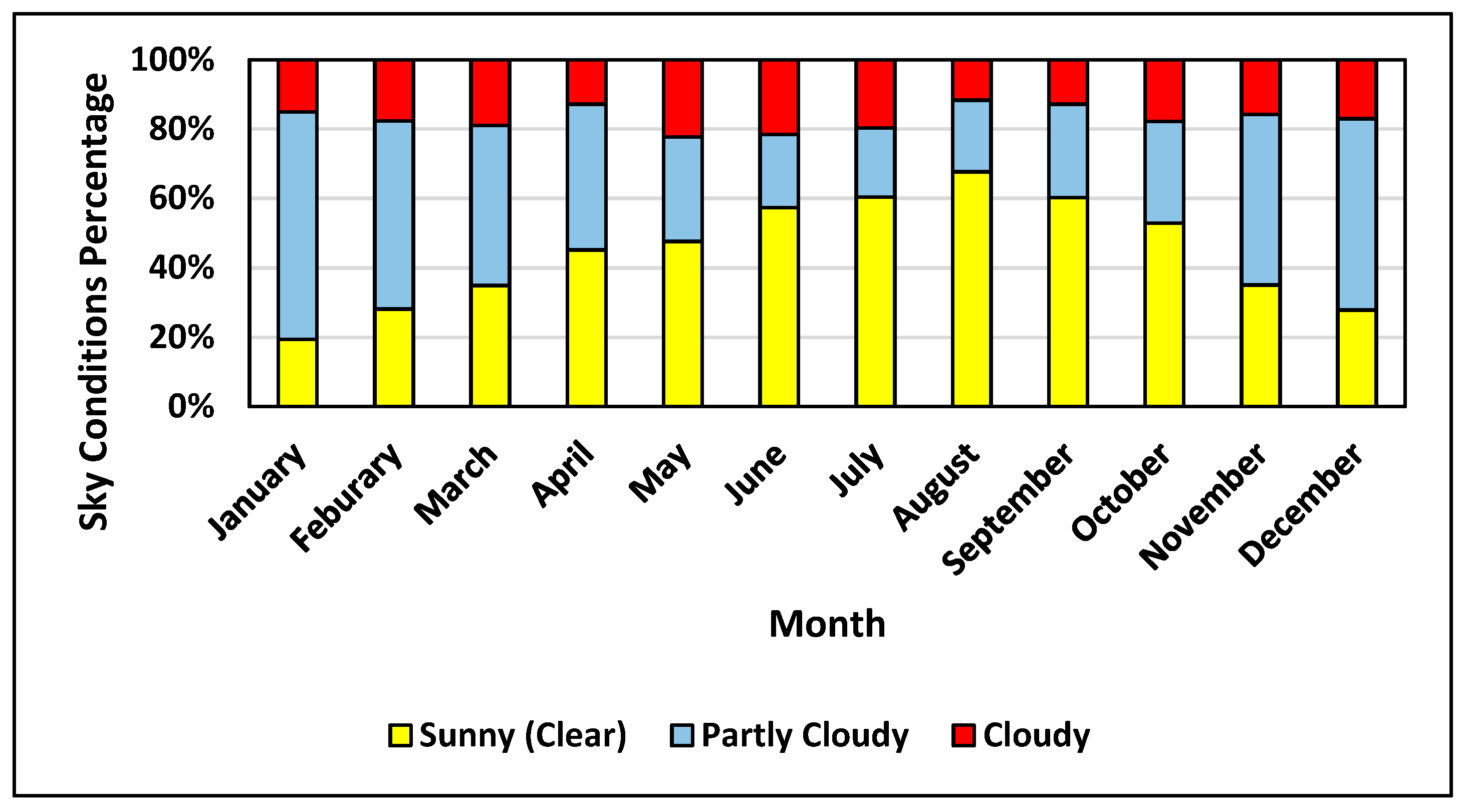
Sky Condition	${\mathbf{k}}_{\mathbf{t}}$
Cloudy	<0.3
Partly cloudy	0.3 ≤ ${\mathrm{k}}_{\mathrm{t}}$≤ 0.5
Sunny	>0.5

[89]:

The results of calculating ${\mathrm{k}}_{\mathrm{t}}$ between 1991–2010 have shown an acceptable coincide comparing to ${\mathrm{k}}_{\mathrm{t}}$ values, which were determined between 1952–1975 by Solar Energy Information Data Bank (SEIDB) [90], as shown in Figure 5.

The analysis of the monthly-average hourly clearness index through the classification of the clearness index level shows that more than 80% of the days could be defined as either sunny or partly cloudy and less than 20% of the days were classified as cloudy. It was also noted that the individual monthly sky conditions percentage of sunny daytime hours exceeded 40% from April through to September, while the percentage of cloudy daytime hours did not exceed about 20%. Consequently, the most significant component of solar radiation for concentrated solar collectors’ performance was the direct normal irradiance (DNI), which was reduced dramatically with growing cloud cover. Concentrating solar collectors could operate efficiently under clear sky conditions of months between June–October that had more than 50% of the sunny daytime hours with hourly ${\mathrm{k}}_{\mathrm{t}}$ values exceeding 0.5 and these collectors were less efficient for the rest months of the year with increasing percentage of partially or completely cloudy daytime hours as shown in Figure 6.

According to the comprehensive analyses of Section 3.1 and Section 5, the operational period of the system could be partitioned into two periods based upon solar radiation intensity: A relatively high-intensity between May–October and a low-intensity from November through to April. Thus, the implementation of calculating the useful (net) solar thermal power that was produced by the solar field requires using a statistical analysis to find the probability distribution density (PDF) and the cumulative probability distribution (CDF) for obtained data of direct normal irradiance, solar incidence angle, and dry bulb temperature, which represent uncertain parameters as in Figure 7, These analyses can be used in the three-point approximation technique to generate a few representative values (discrete points) and their identified probabilities, which are given in

Table 1. Continuous distributions and discrete approximations of uncertain parameters.

Parameter	Continuous Distribution	Discrete Approximation
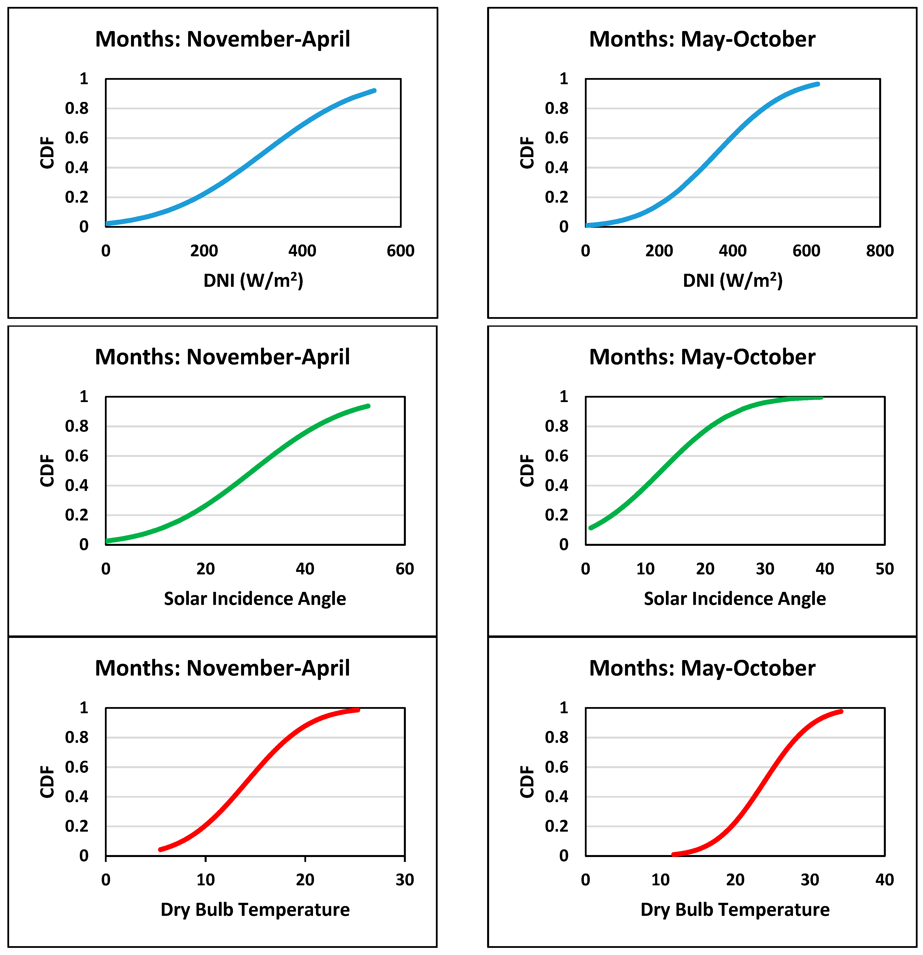
Direct normal irradiance (W/m2) (Months: November–April)	θ$~\mathrm{N}\left(\mathsf{\mu },\mathsf{\sigma }\right)~\mathrm{N}\left(321.1,159.3\right)$	Points: (59.3, 323.7, 555.2) Probabilities: (0.185, 0.630, 0.185)
Direct normal irradiance (W/m2) (Months: May–October)	θ$~\mathrm{N}\left(\mathsf{\mu }, \mathsf{\sigma }\right)~\mathrm{N}\left(356.0,196.4\right)$	Points: (109.8, 356., 605.1) Probabilities: (0.185, 0.630, 0.185)
Solar incidence angle (Months: November–April)	θ$~\mathrm{N}\left(\mathsf{\mu },\mathsf{\sigma }\right)~N\left(29.4, 15.1\right)$	Points: (4.4, 29.5, 53.1) Probabilities: (0.185, 0.630, 0.185)
Solar incidence angle (Months: May–October)	θ$~\mathrm{N}\left(\mathsf{\mu },\mathsf{\sigma }\right)~N\left(12.6, 9.8\right)$	Points: (−2.2, 12.7, 29.7) Probabilities: (0.185, 0.630, 0.185)
Dry bulb temperature (Months: November–April)	θ$~\mathrm{N}\left(\mathsf{\mu },\mathsf{\sigma }\right)~N\left(14.1, 5.0\right)$	Points: (5.7, 14, 22.4) Probabilities: (0.185, 0.630, 0.185)
Dry bulb temperature (Months: May–October)	θ$~\mathrm{N}\left(\mathsf{\mu },\mathsf{\sigma }\right)~N\left(23.8, 5.1\right)$	Points: (15.4, 23.9, 32.3) Probabilities: (0.185, 0.630, 0.185)
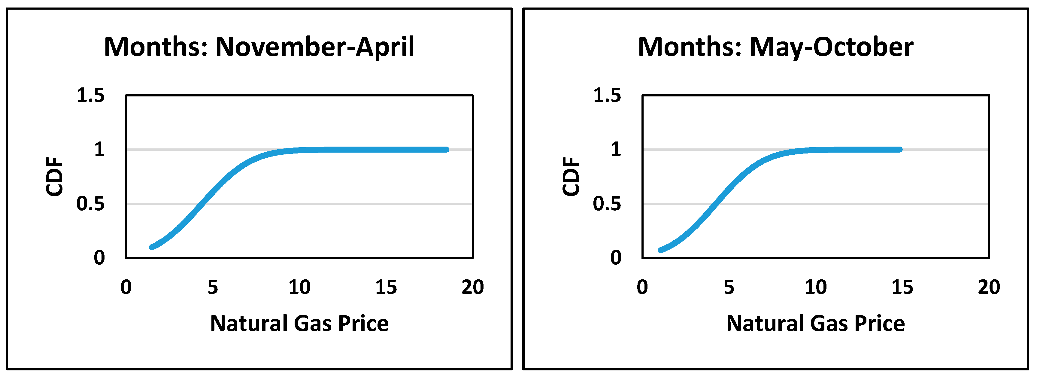
Natural gas price (Months: November–April)	θ$~\mathrm{N}\left(\mathsf{\mu },\mathsf{\sigma }\right)~N\left(4.3, 2.2\right)$	Points: (0.91, 4.3, 8.0) Probabilities: (0.185, 0.630, 0.185)
Natural gas price (Months: May–October)	θ$~\mathrm{N}\left(\mathsf{\mu },\mathsf{\sigma }\right)~N\left(4.2, 2.1\right)$	Points: (0.5, 4.2, 7.7) Probabilities: (0.185, 0.630, 0.185)

. The discrete points were introduced into a detailed performance model of the parabolic trough to provide the useful thermal power values of solar energy to the objective function of the stochastic model along with considering the characteristics of the LS-3 collector chosen and all types of thermal losses (convection, conduction, and radiation) in the solar collection system. The data of natural gas price ($/MMBTU) was obtained from the Energy Information Administration (EIA) [91] for the period between 1997–2018. Based on a specific time of the year, the data of natural gas price was analyzed by using a similar methodology as which has been used to generate representative points for solar energy, as shown in Figure 8.

The determination of minimum utility targets of the conventional fractionation process, which is shown in Figure 9, requires estimating heat duties for reboilers and condensers, in addition, to their stream’s temperature. Therefore, the process was simulated using ASPEN Plus^® for the feed stream condition and composition. The key results of the simulation such as the stream data, heat duty, and stream temperature were summarized in

Table 2. Number of stages and heat exchangers data in each column.

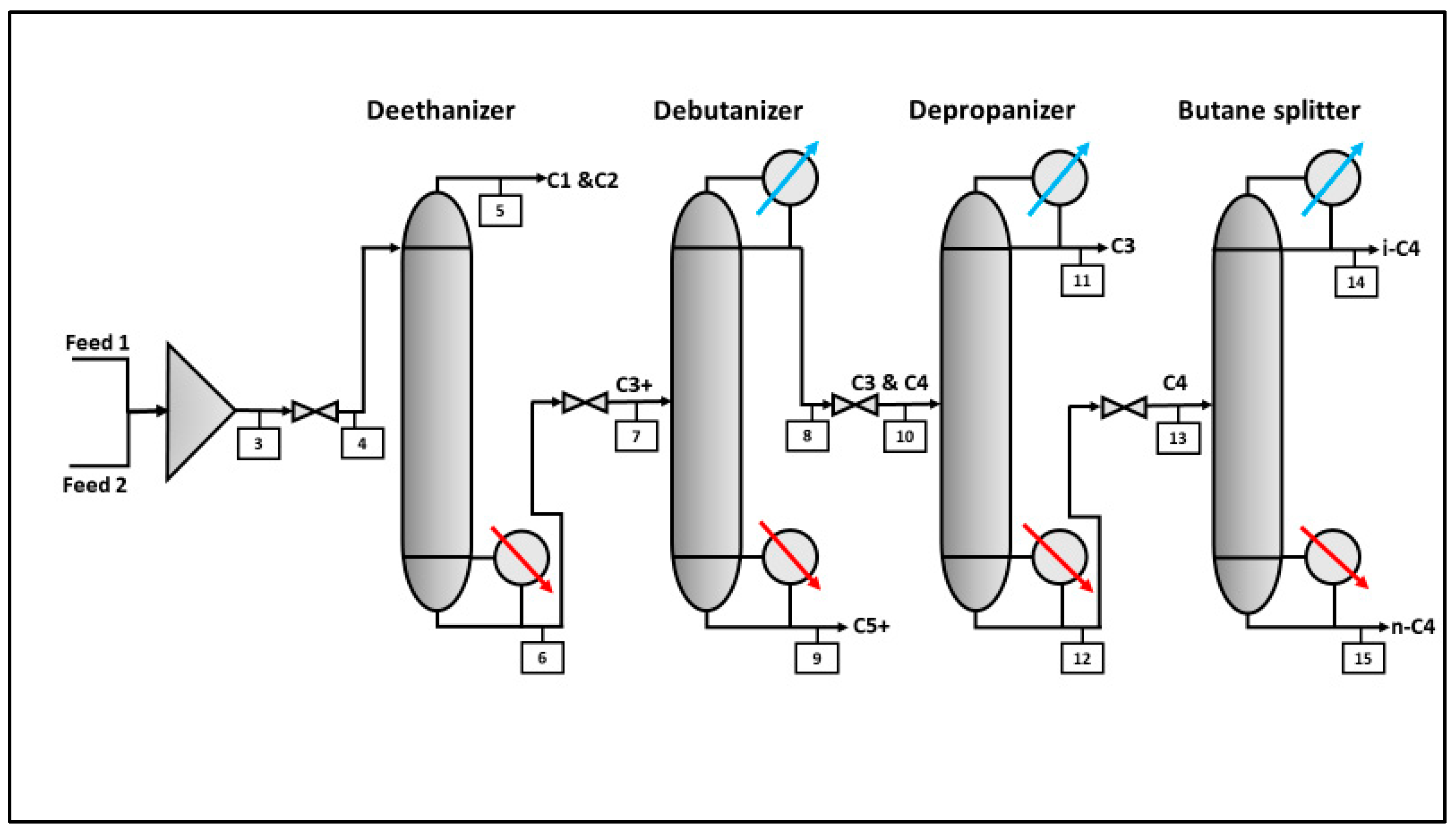
Description	Number of Trays	Reboiler Duty (kW)	Inlet Temperature of Reboiler (°C)	Outlet Temperature of Reboiler (°C)	Condenser Duty (kW)	Inlet Temperature of Condenser (°C)	Outlet Temperature of Condenser (°C)
Deethanizer	19	5587.1	189.7	246.6
Debutanizer	19	735.5	228.2	244.3	−861.55	72.5	61.4
Depropanizer	19	247.99	75.3	77.6	−255.13	23.2	22.7
Butane Splitter	30	185.92	63.2	65.2	−190.74	30.5	29.1

and

Table 3. Stream data for the fractionation process.

Stream Change	Flowrate X Specific Heat (kW/°K)	Supply Temperature (°K)	Target Temperature (°K)	Enthalpy (kW)
H1	78.32	346	335	−861.55
H2	255.13	297	296	−255.13
H3	95.37	304	302	−190.74
HU	?	525	522	?
C1	98.01	463	520	5587.1
C2	45.97	501	517	735.5
C3	82.66	348	351	247.99
C4	92.96	336	338	185.92
CU	?	291	292	?

.

Heat integration was carried out to identify the minimum utility targets through the thermal pinch analysis. The supply temperature, target temperature, and utility for each hot and cold stream of the process are provided in Table 3. The grand composite curve (GCC) was developed for screening utilities to reduce the operating cost as shown in Figure 10.

The optimization formulations of the integrated system were solved for a case study by using the proposed approach, which is described in Section 3, to obtain the optimal design and operation under uncertainty. The stochastic optimization problem was formulated as a multi-scenario mixed integer non-linear programming (MINLP) problem that is a deterministic equivalent of a two-stage stochastic programming model with recourse and solved using the software LINGO^® [76] and MS-Excel 2016 on Intel Core i7-6700 CPU with 16 GB RAM.

The iterative discretization method was presented to realize a significant reduction in the complexity solving of the optimization problem. Thus, in addition to discretize the percentage contribution of RO and MED in the total desalinated water production iteratively, the percentage contribution of solar energy in the total thermal power mix of the system was also iteratively discretized that allows designing the RO and MED separately and to estimate the economic feasibility of integrating solar energy in the system. The objective function was solved to obtain the expected value of the maximum annual net (after-tax) profit by postulating a finite number of scenarios to characterize the uncertain parameters of direct solar irradiance and natural gas price, which take a finite set of known values with their assigned probabilities, as given in Table 1. The probability of each scenario in the final scenario tree equals the product of probabilities of all points that compose it. Consequently, 81 uncertain scenarios were generated by considering the available data of uncertain parameters during the seasonal periods of the year to find a solution for each case individually. A comprehensive study was performed based on economic and sustainability metrics to demonstrate the potential of the proposed system in attaining the profitability and sustainability in the framework of water-energy nexus. The optimization results for all cases are summarized in

Table 4. Economic and sustainability metrics of the system.

(%RO,%MED) *	(25% Solar Energy, 75% Fossil Fuel) **
	TAC	TAP	ROI	PBP
	(MMUSD)	(MMUSD)	%	(year)
30 RO, 70 MED	76.4	100	18.6	5.1
50 RO, 50 MED	73.6	99	18.4	4.4
70 RO, 30 MED	70.9	97.6	18.3	4.5
(%RO,%MED) *	(50% Solar Energy, 50% Fossil Fuel) **
	TAC	TAP	ROI	PBP
	(MMUSD)	(MMUSD)	%	(year)
30 RO, 70 MED	86.6	97.5	17	4.9
50 RO, 50 MED	75.2	97.9	17.1	4.8
70 RO, 30 MED	71.1	95.2	17.3	4.8
(%RO,%MED) *	(75% Solar Energy, 25% Fossil Fuel) **
	TAC	TAP	ROI	PBP
	(MMUSD)	(MMUSD)	%	(year)
30 RO, 70 MED	89.2	101	15.5	5.3
50 RO, 50 MED	84	100	16.1	4.9
70 RO, 30 MED	78.8	98.4	16.3	5.1

* The percentage contribution of reverse osmosis (RO) and multi-effect distillation (MED) in the total desalinated water production. ** The percentage contribution of solar energy and fossil fuel in the total thermal power mix of the system.

.

Based on the above-mentioned results, it can be observed that the system was offered a significant performance through using return on investment (ROI) and payback period (PBP) calculations for the different percentage contributions of RO, MED, solar energy, and fossil fuel. Additionally, the total annual cost (TAC) of the system could be reduced by increasing the percentage contribution of RO over MED and decreasing the percentage contribution of solar energy. This reduction in the total annual cost was based on two reasons: The high capital investment and operating cost of MED, the competitive price of fossil fuels comparing to the relatively high cost of concentrated solar technologies, especially, in the short term. However, the incorporation of solar energy in the system was feasible economically and it would be more feasible in the long-term because of the exhaustion of fossil fuels resources and the diminishing in solar technologies cost.

A comparative study was carried out between the obtained solutions of the stochastic model and those were obtained from the deterministic model with considering the specific percentage contribution of solar energy and fossil fuels (50% solar energy, 50% fossil fuels) and the various percentage of RO and MED contributions, as shown in Figure 11. This study indicated that the solving of the stochastic model offered a significant improvement on values of ROI and PBP comparing with the obtained values of the deterministic model, whereas the total annual costs of the system that were obtained from solving the stochastic model were notably less than obtained from the deterministic model.

It is worth noting that the optimal solution of the system under uncertainty comparatively deviated from the deterministic solution due to considering the uncertain parameters. The relative differences between the stochastic and deterministic cases stem from the capability of the system to meet its demand from thermal power during the operational period by adjustment of the diurnal fluctuations of solar energy through utilizing fossil fuels and thermal energy storage system that make the system works in a nearly steady mode and inherits robustness against the uncertainty. However, there is still a necessity to handle the uncertain nature of the actual hourly, daily, and seasonal data by developing the system design and operation under uncertainty that can address operational issues and provide the detailed design. These concepts are consistent with the objective of this work to start preliminary screening and then determine main targets that can be as a guide to the proper design and operation for the system.

In order to evaluate the impact of the system performance on the environmental aspects, a comprehensive comparison has been achieved for the amount CO₂, which can be reduced during the operational mode for the system, as described in Figure 12.

The comparison indicated obviously that the enhancement in the environmental performance of the system requires increasing the percentage of solar energy contribution and RO contribution because the RO plant consumes less thermal power than MED plant and solar energy can be contributed to meet a demand of MED plant from the thermal power and lessen fossil fuel consumption, which causes sustaining fossil fuels resources and significantly diminishing in the emissions of greenhouse gases. Consequently, reconciliation of economic and environmental objectives is indispensable to attaining the optimal configuration of the system, which operates under uncertainty conditions through using a sustainability weighted return on investment calculation [77,78]. Additionally, flared gas can be converted from the source of greenhouse gas emissions in a shale gas site to one of the energy sources that may be contributing effectively to improve the economic and environmental performance of the system [13,92].

6. Conclusions

A new hierarchical procedure was developed for formulating and optimizing an integrated system operating under uncertainty to address the problem of water-energy nexus in the shale gas and oil production sites. The system utilized a hybrid of fossil fuel and solar energy to enhance the sustainable design of the system that consisted of the following key elements: Concentrated solar collectors, thermal energy storage, cogeneration process, MED, and RO. An industrial process (fractionation process) was incorporated into the system to satisfy heating and cooling demands of the process. The optimization problem was formulated as a multi-scenario MINLP problem that was a deterministic equivalent of a two-stage stochastic programming model to characterize the uncertainty in the system by considering two uncertain operational parameters (normal direct irradiance, and fossil fuel price). Solar energy was included as a source of thermal power for the entire system through the heat recovery system (steam generator). The heat integration technique was carried out for hot and cold streams of the fractionation process to determine the surplus and deficit energy content in addition to the quality of hot and cold streams temperature. The operational period was discretized based on two seasons of the year to create a finite number of scenarios for uncertain parameters. The percentage of incorporating water treatment technologies and solar energy into the system was iteratively discretized. The results from solving a case study for Eagle Ford Basin in Texas indicated the applicability of the integrated approach based on stochastic optimization to show the system’s economic and environmental merits in solving the problem of water management in shale gas production using a water-energy nexus framework and incorporating renewables.

References

- Al-Douri, A.; Sengupta, D.; El-Halwagi, M.M. Shale Gas Monetization—A Review of Downstream Processing to Chemicals and Fuels. J. Nat. Gas Sci. Eng. 2017, 45, 436–455. [Google Scholar] [CrossRef]
- Energy Information Administration. Available online: https://www.eia.gov/todayinenergy/detail.php?id=38372 (accessed on 13 July 2019).
- Zhang, C.; El-Halwagi, M.M. Estimate the Capital Cost of Shale-Gas Monetization Projects. Chem. Eng. Prog. 2017, 113, 28–32. [Google Scholar]
- Ortiz-Espinoza, A.P.; Noureldin, M.M.; El-Halwagi, M.M.; Jiménez-Gutiérrez, A. Design, simulation and techno-economic analysis of two processes for the conversion of shale gas to ethylene. Comput. Chem. Eng. 2017, 107, 237–246. [Google Scholar] [CrossRef]
- Pérez-Uresti, S.; Adrián-Mendiola, J.; El-Halwagi, M.; Jiménez-Gutiérrez, A. Techno-Economic Assessment of Benzene Production from Shale Gas. Processes 2017, 5, 33. [Google Scholar] [CrossRef]
- Julián-Durán, L.M.; Ortiz-Espinoza, A.P.; El-Halwagi, M.M.; Jiménez-Gutiérrez, A. Techno-economic assessment and environmental impact of shale gas alternatives to methanol. ACS Sustain. Chem. Eng. 2014, 2, 2338–2344. [Google Scholar] [CrossRef]
- Kondash, A.J.; Albright, E.; Vengosh, A. Quantity of flowback and produced waters from unconventional oil and gas exploration. Sci. Total Environ. 2017, 574, 314–321. [Google Scholar] [CrossRef] [Green Version]
- Oke, D.; Majozi, T.; Mukherjee, R.; Sengupta, D.; El-Halwagi, M.M. Simultaneous Energy and Water Optimization in Shale Exploration. Processes 2018, 6, 86. [Google Scholar] [CrossRef]
- Jiang, M.; Hendrickson, C.T.; VanBriesen, J.M. Life cycle water consumption and wastewater generation impacts of a Marcellus shale gas well. Environ. Sci. Technol. 2014, 48, 1911–1920. [Google Scholar] [CrossRef]
- Guerra, O.J.; Calderón, A.J.; Papageorgiou, L.G.; Siirola, J.J.; Reklaitis, G.V. An optimization framework for the integration of water management and shale gas supply chain design. Comput. Chem. Eng. 2016, 92, 230–255. [Google Scholar] [CrossRef]
- Elsayed, N.A.; Barrufet, M.A.; Eljack, F.T.; El-Halwagi, M.M. Optimal design of thermal membrane distillation systems for the treatment of shale gas flowback water. Int. J. Membr. Sci. Technol. 2015, 2, 1–9. [Google Scholar]
- Yang, L.; Grossmann, I.E.; Manno, J. Optimization models for shale gas water management. AIChE J. 2014, 60, 3490–3501. [Google Scholar] [CrossRef]
- Al-Aboosi, F.Y.; El-Halwagi, M.M. An Integrated Approach to Water-Energy Nexus in Shale-Gas Production. Processes 2018, 6, 52. [Google Scholar] [CrossRef]
- Oke, D.; Mukherjee, R.; Sengupta, D.; Majozi, T.; El-Halwagi, M.M. Optimization of water-energy nexus in shale gas exploration: From production to transmission. Energy 2019, 183, 651–669. [Google Scholar] [CrossRef]
- El-Halwagi, M.M. A Shortcut Approach to the Design of Once-Through Multi-Stage Flash Desalination Systems. Desalin. Water Treat. 2017, 62, 43–56. [Google Scholar] [CrossRef]
- Gabriel, K.; El-Halwagi, M.M.; Linke, P. Optimization Across Water-Energy Nexus for Integrating Heat, Power, and Water for Industrial Processes Coupled with Hybrid Thermal-Membrane Desalination. Ind. Eng. Chem. Res. 2016, 55, 3442–3466. [Google Scholar] [CrossRef]
- Bhojwani, S.; Topolski, K.; Mukherjee, R.; Sengupta, D.; El-Halwagi, M. Technology Review and Data Analysis for Cost Assessment of Water Treatment Systems. Sci. Total Environ. 2019, 651, 2749–2761. [Google Scholar] [CrossRef]
- Saif, Y.; Elkamel, A.; Pritzker, M. Global optimization of reverse osmosis network for wastewater treatment and minimization. Ind. Eng. Chem. Res. 2008, 47, 3060–3070. [Google Scholar] [CrossRef]
- El-Halwagi, M.M. Synthesis of Optimal Reverse-Osmosis Networks for Waste Reduction. AIChE J. 1992, 38, 1185–1198. [Google Scholar] [CrossRef]
- Khor, C.S.; Foo, D.C.Y.; El-Halwagi, M.M.; Tan, R.R.; Shah, N. A Superstructure Optimization Approach for Membrane Separation-Based Water Regeneration Network Synthesis with Detailed Nonlinear Mechanistic Reverse Osmosis Model. Ind. Eng. Chem. Res. 2011, 50, 13444–13456. [Google Scholar] [CrossRef]
- Al-Azri, N.; Al-Thubaiti, M.; El-Halwagi, M. An algorithmic approach to the optimization of process cogeneration. Clean Technol. Environ. Policy 2009, 11, 329–338. [Google Scholar] [CrossRef]
- Mavromatis, S.; Kokossis, A. Conceptual optimisation of utility networks for operational variations—I. Targets and level optimisation. Chem. Eng. Sci. 1998, 53, 1585–1608. [Google Scholar] [CrossRef]
- Mohan, T.; El-Halwagi, M.M. An algebraic targeting approach for effective utilization of biomass in combined heat and power systems through process integration. Clean Technol. Environ. Policy 2007, 9, 13–25. [Google Scholar] [CrossRef]
- El-Halwagi, M.; Harell, D.; Spriggs, H.D. Targeting cogeneration and waste utilization through process integration. Appl. Energy 2009, 86, 880–887. [Google Scholar] [CrossRef]
- Lira-Barragán, L.F.; Ponce-Ortega, J.M.; Guillén-Gosálbez, G.; El-Halwagi, M.M. Optimal water management under uncertainty for shale gas production. Ind. Eng. Chem. Res. 2016, 55, 1322–1335. [Google Scholar] [CrossRef]
- Khor, C.S.; Elkamel, A.; Ponnambalam, K.; Douglas, L. Two-stage stochastic programming with fixed recourse via scenario planning with economic and operational risk management for petroleum refinery planning under uncertainty. Chem. Eng. Process. Process Intensif. 2008, 47, 1744–1764. [Google Scholar] [CrossRef]
- Sharif, A.; Almansoori, A.; Fowler, M.; Elkamel, A.; Alrafea, K. Design of an energy hub based on natural gas and renewable energy sources. Int. J. Energy Res. 2014, 38, 363–373. [Google Scholar] [CrossRef]
- Tora, E.A.; El-Halwagi, M.M. Integrated conceptual design of solar-assisted trigeneration systems. Comput. Chem. Eng. 2011, 35, 1807–1814. [Google Scholar] [CrossRef]
- Chebeir, J.; Geraili, A.; Romagnoli, J. Development of Shale Gas Supply Chain Network under Market Uncertainties. Energies 2017, 10, 246. [Google Scholar] [CrossRef]
- Steimel, J.; Engell, S. Conceptual design and optimization of chemical processes under uncertainty by two-stage programming. Comput. Chem. Eng. 2015, 81, 200–217. [Google Scholar] [CrossRef]
- Shafiee, S.; Topal, E. A long-term view of worldwide fossil fuel prices. Appl. Energy 2010, 87, 988–1000. [Google Scholar] [CrossRef]
- Mirkhani, S.; Saboohi, Y. Stochastic modeling of the energy supply system with uncertain fuel price–A case of emerging technologies for distributed power generation. Appl. Energy 2012, 93, 668–674. [Google Scholar] [CrossRef]
- Rogers, J. Strategy, Value and Risk: The Real Options Approach; Springer: Berlin/Heidelberg, Germany, 2009. [Google Scholar]
- Geiger, A. Strategic Power Plant Investment Planning under Fuel and Carbon Price Uncertainty; KIT Scientific Publishing: Karlsruhe, Germany, 2011. [Google Scholar]
- Iyer, R.; Grossmann, I.E. Synthesis and operational planning of utility systems for multiperiod operation. Comput. Chem. Eng. 1998, 22, 979–993. [Google Scholar] [CrossRef]
- Carpaneto, E.; Chicco, G.; Mancarella, P.; Russo, A. Cogeneration planning under uncertainty: Part I: Multiple time frame approach. Appl. Energy 2011, 88, 1059–1067. [Google Scholar] [CrossRef]
- Carpaneto, E.; Chicco, G.; Mancarella, P.; Russo, A. Cogeneration planning under uncertainty. Part II: Decision theory-based assessment of planning alternatives. Appl. Energy 2011, 88, 1075–1083. [Google Scholar] [CrossRef]
- Sun, L.; Gai, L.; Smith, R. Site utility system optimization with operation adjustment under uncertainty. Appl. Energy 2017, 186, 450–456. [Google Scholar] [CrossRef]
- Bamufleh, H.; Abdelhady, F.; Baaqeel, H.M.; El-Halwagi, M.M. Optimization of multi-effect distillation with brine treatment via membrane distillation and process heat integration. Desalination 2017, 408, 110–118. [Google Scholar] [CrossRef]
- El-Halwagi, M.M. Sustainable Design through Process Integration: Fundamentals and Applications to Industrial Pollution Prevention, Resource Conservation, and Profitability Enhancement; Butterworth-Heinemann: New York, NY, USA, 2017. [Google Scholar]
- Ioannou, A.; Fuzuli, G.; Brennan, F.; Yudha, S.W.; Angus, A. Multi-stage stochastic optimization framework for power generation system planning integrating hybrid uncertainty modelling. Energy Econom. 2019, 80, 760–776. [Google Scholar] [CrossRef]
- Brown, S.; Yucel, M.K. what drives natural gas prices? Energy J. 2008, 29, 45. [Google Scholar] [CrossRef]
- Pfeifer, E.; Bodily, S.E.; Frey, S.C., Jr. Pearson-Tukey Three-Point Approximations Versus Monte Carlo Simulation. Decis. Sci. 1991, 22, 74–90. [Google Scholar] [CrossRef]
- Miller, A.C., III; Rice, T.R. Discrete approximations of probability distributions. Manag. Sci. 1983, 29, 352–362. [Google Scholar] [CrossRef]
- Keefer, D.L.; Bodily, S.E. Three-point approximations for continuous random variables. Manag. Sci. 1983, 29, 595–609. [Google Scholar] [CrossRef]
- Hammond, R.K.; Bickel, J.E. Reexamining discrete approximations to continuous distributions. Decis. Anal. 2013, 10, 6–25. [Google Scholar] [CrossRef]
- Woodruff, J.; Dimitrov, N.B. Optimal discretization for decision analysis. Oper. Res. Perspect. 2018, 5, 288–305. [Google Scholar] [CrossRef]
- DeCoursey, W. Statistics and Probability for Engineering Applications; Elsevier: Amsterdam, The Netherlands, 2003. [Google Scholar]
- Mavromatidis, G.; Orehounig, K.; Carmeliet, J. Design of distributed energy systems under uncertainty: A two-stage stochastic programming approach. Appl. Energy 2018, 222, 932–950. [Google Scholar] [CrossRef]
- Dupačová, J.; Kozmík, V. SDDP for multistage stochastic programs: Preprocessing via scenario reduction. Comput. Manag. Sci. 2017, 14, 67–80. [Google Scholar] [CrossRef]
- Pranevicius, H.; Sutiene, K. Scenario tree generation by clustering the simulated data paths. In Proceedings of the 21st European Conference on Modelling and Simulation, Prague, Czech Republic, 4–6 June 2007. [Google Scholar]
- Khatami, M.; Mahootchi, M.; Farahani, R.Z. Benders’ decomposition for concurrent redesign of forward and closed-loop supply chain network with demand and return uncertainties. Transp. Res. Part E Logist. Transp. Rev. 2015, 79, 1–21. [Google Scholar] [CrossRef]
- Mavromatidis, G.; Orehounig, K.; Carmeliet, J. Trade-offs between risk-neutral and risk-averse decision making for the design of distributed energy systems under uncertainty. Proceedings of ECOS 2017—The 30th International Conference on Efficiency, Cost, Optimization, Simulation and Environmental Impact of Energy Systems, San Diego, CA, USA, 2–6 July 2017. [Google Scholar]
- Hasani, A. Two-stage Stochastic Programing Based on the Accelerated Benders Decomposition for Designing Power Network Design under Uncertainty. Int. J. Ind. Eng. Prod. Res. 2017, 28, 163–174. [Google Scholar]
- Acevedo, J.; Pistikopoulos, E.N. Stochastic optimization-based algorithms for process synthesis under uncertainty. Comput. Chem. Eng. 1998, 22, 647–671. [Google Scholar] [CrossRef]
- Karuppiah, R.; Grossmann, I.E. Global optimization of multiscenario mixed integer nonlinear programming models arising in the synthesis of integrated water networks under uncertainty. Comput. Chem. Eng. 2008, 32, 145–160. [Google Scholar] [CrossRef] [Green Version]
- Paules, G., IV; Floudas, C. Stochastic programming in process synthesis: A two-stage model with MINLP recourse for multiperiod heat-integrated distillation sequences. Comput. Chem. Eng. 1992, 16, 189–210. [Google Scholar] [CrossRef]
- Clay, R.; Grossmann, I. A disaggregation algorithm for the optimization of stochastic planning models. Comput. Chem. Eng. 1997, 21, 751–774. [Google Scholar] [CrossRef]
- Ierapetritou, M.G.; Acevedo, J.; Pistikopoulos, E. An optimization approach for process engineering problems under uncertainty. Comput. Chem. Eng. 1996, 20, 703–709. [Google Scholar] [CrossRef]
- Goswami, D.Y.; Kreith, F. Energy Conversion; CRC Press: Boca Raton, FL, USA, 2007. [Google Scholar]
- Mittelman, G.; Epstein, M. A novel power block for CSP systems. Sol. Energy 2010, 84, 1761–1771. [Google Scholar] [CrossRef]
- Channiwala, S.; Ekbote, A. A generalized model to estimate field size for solar-only parabolic trough plant. In Proceedings of the 3rd Southern African Solar Energy Conference, Kruger National Park, South Africa, 11–13 May 2015. [Google Scholar]
- Eck, M.; Hirsch, T.; Feldhoff, J.F.; Kretschmann, D.; Dersch, J.; Morales, A.G.; Gonzalez-Martinez, L.; Bachelier, C.; Platzer, W.; Riffelmann, K.-J.; et al. Guidelines for CSP yield analysis—Optical losses of line focusing systems; definitions, sensitivity analysis and modeling approaches. Energy Procedia 2014, 49, 1318–1327. [Google Scholar] [CrossRef]
- Alnouri, S.Y.; Linke, P.; El-Halwagi, M.M. Synthesis of industrial park water reuse networks considering treatment systems and merged connectivity options. Comput. Chem. Eng. 2016, 91, 289–306. [Google Scholar] [CrossRef]
- Bamufleh, H.S.; Ponce-Ortega, J.M.; El-Halwagi, M.M. Multi-objective optimization of process cogeneration systems with economic, environmental, and social tradeoffs. Clean Technol. Environ. Policy 2013, 15, 185–197. [Google Scholar] [CrossRef]
- Branan, C. Rules of Thumb for Chemical Engineers: A Manual of Quick. In Accurate Solutions to Everyday Process Engineering Problems, 3rd ed.; Gulf Professional Pub.: Amsterdam, The Netherlands, 2002. [Google Scholar]
- Kumana, J. How to Calculate the True Cost of Steam; DOE/GO-102003-1736; US Department of Energy: Washington, DC, USA, 2003.
- National Renewable Energy Laboratory. Assessment of Parabolic Trough and Power Tower Solar Technology Cost and Performance Forecasts; DIANE Publishing: Collingdale, PA, USA, 2003. [Google Scholar]
- Philibert, C. Technology Roadmap: Concentrating Solar Power; OECD/IEA: Paris Cedex, France, 2010. [Google Scholar]
- Dale, M. A comparative analysis of energy costs of photovoltaic, solar thermal, and wind electricity generation technologies. Appl. Sci. 2013, 3, 325–337. [Google Scholar] [CrossRef]
- Alnouri, S.Y.; Linke, P. Optimal SWRO desalination network synthesis using multiple water quality parameters. J. Membr. Sci. 2013, 444, 493–512. [Google Scholar] [CrossRef]
- Gabriel, K.J.; Linke, P.; El-Halwagi, M.M. Optimization of multi-effect distillation process using a linear enthalpy model. Desalination 2015, 365, 261–276. [Google Scholar] [CrossRef]
- Atilhan, S. A Systems-Integration Approach to the Optimal Design and Operation of Macroscopic Water Desalination and Supply Networks; Texas A&M University: College Station, TX, USA, 2011. [Google Scholar]
- Recovery, L.; Khabibullin, E.; Febrianti, F.; Sheng, J.; Bandyopadhyay, S.; Skogestad, S. (Eds.) TKP4170 Process Design; Project: Trondheim, Norway, 2010. [Google Scholar]
- Kaplan, R.; Mamrosh, D.; Salih, H.H.; Dastgheib, S.A. Assessment of desalination technologies for treatment of a highly saline brine from a potential CO2 storage site. Desalination 2017, 404, 87–101. [Google Scholar] [CrossRef]
- Schrage, L. Optimization Modeling with LINGO; LINDO Systems Inc.: Chicago, IL, USA, 2006. [Google Scholar]
- El-Halwagi, M.M. A Return on Investment Metric for Incorporating Sustainability in Process Integration and Improvement Projects. Clean Technol. Environ. Policy 2017, 19, 611–617. [Google Scholar] [CrossRef]
- Guillen-Cuevas, K.; Ortiz-Espinoza, A.; Ozinan, E.; Jiménez-Gutiérrez, A.; Kazantzis, N.K.; El-Halwagi, M.M. Incorporation of Safety and Sustainability in Conceptual Design via A Return on Investment Metric. ACS Sustain. Chem. Eng. 2018, 6, 1411–1416. [Google Scholar] [CrossRef]
- Mohtar, R.H.; Shafiezadeh, H.; Blake, J.; Daher, B. Economic, social, and environmental evaluation of energy development in the Eagle Ford shale play. Sci. Total Environ. 2019, 646, 1601–1614. [Google Scholar] [CrossRef]
- Trieb, F.; Scharfe, J.; Kern, J.; Nieseor, T.; Glueckstern, P. Combined Solar Power and Desalination Plants: Techno-Economic Potential in Mediterranean Partner Countries; German Aerospace Center (DLR): Stuttgart, Germany, 2009. [Google Scholar]
- Atilhan, S.; Linke, P.; Abdel-Wahab, A.; El-Halwagi, M.M. A systems integration approach to the design of regional water desalination and supply networks. Int. J. Process Syst. Eng. 2011, 1, 125–135. [Google Scholar] [CrossRef]
- Ghaffour, N.; Missimer, T.M.; Amy, G.L. Technical review and evaluation of the economics of water desalination: Current and future challenges for better water supply sustainability. Desalination 2013, 309, 197–207. [Google Scholar] [CrossRef] [Green Version]
- Mezher, T.; Fath, H.; Abbas, Z.; Khaled, A. Techno-economic assessment and environmental impacts of desalination technologies. Desalination 2011, 266, 263–273. [Google Scholar] [CrossRef]
- RPSEA. Advanced Treatment of Shale Gas Fracturing Water to Produce Re-Use or Discharge Quality Water. 2015. Retrieved July, 2019. Available online: https://www.rpsea.org/node/222 (accessed on 13 July 2019).
- Price, H. A parabolic trough solar power plant simulation model. In Proceedings of the ASME International Solar Energy Conference, Kohala Coast, HI, USA, 15–18 March 2003. [Google Scholar]
- Eldar, K.; Feby, F.; Juejing, S. Process Design and Economic Investigation of LPG Production from Natural Gas Liquids (NGL); TKP4170 Process Design: Trondheim, Norway, 2010. [Google Scholar]
- Horwitt, D.; Sumi, L. Up in Flames: US Shale Oil boom comes at Expense of Wasted Natural Gas, Increased CO2; Earthworks: Washington, DC, USA, 2014. [Google Scholar]
- Koudouris, G.; Dimitriadis, P.; Iliopoulou, T.; Mamassis, N.; Koutsoyiannis, D. A stochastic model for the hourly solar radiation process for application in renewable resources management. Adv. Geosci. 2018, 45, 139–145. [Google Scholar] [CrossRef] [Green Version]
- Pavanello, D.; Zaaiman, W.; Colli, A.; Heiser, J.; Smith, S. Statistical functions and relevant correlation coefficients of clearness index. J. Atmos. Sol.-Terrestr. Phys. 2015, 130, 142–150. [Google Scholar] [CrossRef]
- Knapp, C.L.; Stoffel, T.L.; Whitaker, S.S. Insolation Data Manual; US Government Printing Office: Golden, CO, USA, 1980.
- U.S. Department of Energy; Energy Information Administration; Independent Statistics & Analysis. Henry Hub Natural Gas Spot Price. Available online: https://www.eia.gov/dnav/ng/hist/rngwhhdd.htm (accessed on 13 July 2019).
- Tovar-Facio, J.; Eljack, F.; Ponce-Ortega, J.M.; El-Halwagi, M.M. Optimal Design of Multiplant Cogeneration Systems with Uncertain Flaring and Venting. ACS Sustain. Chem. Eng. 2016, 5, 675–688. [Google Scholar] [CrossRef]
- Herrmann, U.; Kelly, B.; Price, H. Two-tank molten salt storage for parabolic trough solar power plants. Energy 2004, 29, 883–893. [Google Scholar] [CrossRef]