Article

Observed Daily Profiles of Polyaromatic Hydrocarbons and Quinones in the Gas and PM1 Phases: Sources and Secondary Production in a Metropolitan Area of Mexico

by
Valeria Ojeda-Castillo
1,2,
Iván Y. Hernández-Paniagua
3,
Leonel Hernández-Mena
1,
Alberto López-López
1,†,
José de Jesús Díaz-Torres
1,
Sergio Alonso-Romero
4 and
Jorge del Real-Olvera
1,*
1
Unidad de Tecnología Ambiental, Centro de Investigación y Asistencia en Tecnología y Diseño del Estado de Jalisco A.C. (CIATEJ), Av. Normalistas 800, Col. Colinas de la Normal, Guadalajara-Jalisco C.P. 44270, Mexico
2
Departamento de Investigación, Centro Universitario UTEG A.C., Av. Héroes Ferrocarrileros 1325, Col. La Aurora, Guadalajara-Jalisco C.P. 44460, Mexico
3
CONACYT-Centro de Investigación en Geografía y Geomática “Ing. Jorge L. Tamayo” A.C., Contoy 137, Lomas de Padierna, Tlalpan, Ciudad de México C.P. 14240, Mexico
4
Investigación en Materiales, Centro de Innovación Aplicada en Tecnologías Competitivas A.C. (CIATEC), Boulevard Omega 201, Col. Industrial Delta, León-Guanajuato C.P. 37545, Mexico
*
Author to whom correspondence should be addressed.
Deceased.
Sustainability 2019, 11(22), 6345; https://doi.org/10.3390/su11226345
Submission received: 8 September 2019 / Revised: 4 November 2019 / Accepted: 8 November 2019 / Published: 12 November 2019
(This article belongs to the Special Issue Sustainable Air Pollution Management)

Abstract

:
The diel variation of meteorological conditions strongly influences the formation processes of secondary air pollutants. However, due to the complexity of sampling highly reactive chemical compounds, significant information about their transformation and source can be lost when sampling over long periods, affecting the representativeness of the samples. In order to determine the contribution of primary and secondary sources to ambient levels of polyaromatic hydrocarbons (PAHs) and quinones, measurements of gas and PM1 phases were conducted at an urban site in the Guadalajara Metropolitan Area (GMA) using a 4-h sampling protocol. The relation between PAHs, quinones, criteria pollutants, and meteorology was also addressed using statistical analyses. Total PAHs (gas phase + PM1 phase) ambient levels ranged between 184.03 ng m−3 from 19:00 to 23:00 h and 607.90 ng m−3 from 07:00 to 11:00 h. These figures both coincide with the highest vehicular activity peak in the morning and at night near the sampling site, highlighting the dominant role of vehicular emissions on PAHs levels. For the gas phase, PAHs ranged from 177.59 to 595.03 ng m−3, while for PM1, they ranged between 4.81 and 17.44 ng m−3. The distribution of the different PAHs compounds between the gas and PM1 phases was consistent with their vapour pressure (p °L) reported in the literature, the PAHs with vapour pressure ≤ 1 × 10⁻³ Pa were partitioned to the PM1, and PAHs with vapour pressures ≥ 1 × 10⁻³ Pa were partitioned to the gas phase. PAHs diagnostic ratios confirmed an anthropogenic emission source, suggesting that incomplete gasoline and diesel combustion from motor vehicles represent the major share of primary emissions. Quinones ambient levels ranged between 18.02 ng m−3 at 19:00–23:00 h and 48.78 ng m−3 at 15:00–19:00 h, with significant increases during the daytime. The distribution of quinone species with vapour pressures (p °L) below 1 × 10⁻⁴ Pa were primarily partitioned to the PM1, and quinones with vapour pressures above 1 × 10⁻⁴ Pa were mainly partitioned to the gas phase. The analysis of the distribution of phases in quinones suggested emissions from primary sources and their consequent degradation in the gas phase, while quinones in PM1 showed mainly secondary formation modulated by UV, temperature, O3, and wind speed. The sampling protocol proposed in this study allowed obtaining detailed information on PAHs and quinone sources and their secondary processing to be compared to existing studies within the GMA.

1. Introduction

Polyaromatic hydrocarbons (PAHs) represent a significant fraction of organic compounds present both in the gas and particulate phases. PAHs are highly toxic, mutagenic, and carcinogenic to microorganisms, as well as to higher forms of life, including humans [1]. Quinones are formed directly from combustion processes as in diesel and gasoline engines, as well as by oxidants in the atmosphere through the gas phase and heterogeneous reactions of PAHs. Hence, the quinones may serve as tracers to identify their emission sources and photochemical pathways [2,3]. They have a central role in allergic airway diseases such as asthma and cardiovascular effects due to their ability to generate oxidative stress, inflammation, and immunomodulating effects in the lungs and airways. The prediction of quinone levels is crucial as existing studies have shown them to be more harmful compounds than their precursors [4,5,6].
It has been reported that about 90%–95% of particulate PAHs are related to particles with an aerodynamic diameter < 3.3 μm, and the maximum distributions are contained between 0.4 and 1.1 μm and may remain in the environment for a long time and have long-range transportation [7]. Additionally, Chen et al. [8] suggested that, with smaller particle size, PM1 is more harmful than PM2.5. Despite this, ambient levels and distribution of quinones have been determined mainly in PM10 [9,10,11] and total suspended particles [12,13], while few studies have addressed those in the gas phase and fine particles simultaneously [14,15,16].
The meteorological conditions (wind speed, wind direction, temperature, relative humidity, absolute humidity, and mixing layer height) often play important roles in local air quality dynamics through pollutant accumulation and diffusion processes, regional transport, and chemical and physical processing (i.e., photolysis, thermal decomposition, wet deposition, particle growth, etc.) that may lead to the formation of secondary species [17,18,19]. Thus, the diel variations of meteorological conditions may strongly influence the concentrations of secondary pollutants [20,21,22,23], which typically increase during periods of enhanced photochemical activity over midday and decrease afterwards due to dilution effects [24].
Since the chemistry in the atmosphere is dynamic, on timescales ranging from seconds to hours, air sampling over long periods (24–48 h) may lead to the loss of significant information about pollutants ambient concentrations due to the rapid changes in the atmospheric composition and the mismatch between the timescales of atmospheric processes and of sampling. Indeed, the loss of that significant information could lead to bias in the quantification of health risk.
Existing studies dealing with organic compounds have estimated that sampling artefacts may significantly affect the representativeness of samples and their quantification, which have been reported in up to −80% for volatilisation-induced bias to +50% for the bias induced by adsorption [21,25,26]. Therefore, sampling artefacts becomes a limiting factor when comparing existing studies of air pollutants due to the high levels of uncertainty in the values reported. As result, artefacts become a limiting factor when comparing different pollutant studies since they have a lot of uncertainty. The complex nature of samples of organic compounds and secondary pollutants and their further analyses have limited the number and length of studies that have addressed diel variability of these chemical species, but have also biased the existing information of secondary formation processes, gas-particle partition, and chain of chemical reactions [27,28].
Air sampling with a shorter time duration may help to obtain significant information to characterise PAHs-derivatives; improving the understanding of secondary chemical processes, behaviour, fate, and conditions that favour the generation of highly toxic compounds, such as quinones [20,29]. Some studies have reported already variations in measurements of PAHs and derivatives (nitro-PAHs and oxy-PAHs) obtained under different time sampling schemes [20,30,31,32,33,34]. In this context, identifying primary sources of quinones and understanding secondary transformation processes, along with their fate routes [35], are essential for reducing population exposure and the effects on public health resulting from this exposure.
To the best of our knowledge, few reports of quinones have considered the emissions of their PAHs precursors in the gas and particulate phases simultaneously. Nevertheless, obtaining information of both the PAHs and quinones can help to extend current knowledge about gas–particle distribution, heterogeneous reactions, the volatilisation and adsorption processes of these species in urban environments. In this study, we address the abundance, atmospheric phase distribution, and diel cycles of parent PAHs and quinones at one urban site within the Guadalajara Metropolitan Area (GMA, the second most populated area in Mexico and an important industrial region). Samples of gas and fine particle phases were collected over periods of 4 h during three consecutive days in order to address primary emissions and secondary sources of PAHs and quinones. To elucidate the quinones main formation pathways, correlation analyses and bivariate polar plots were carried out.

2. Materials and Methods
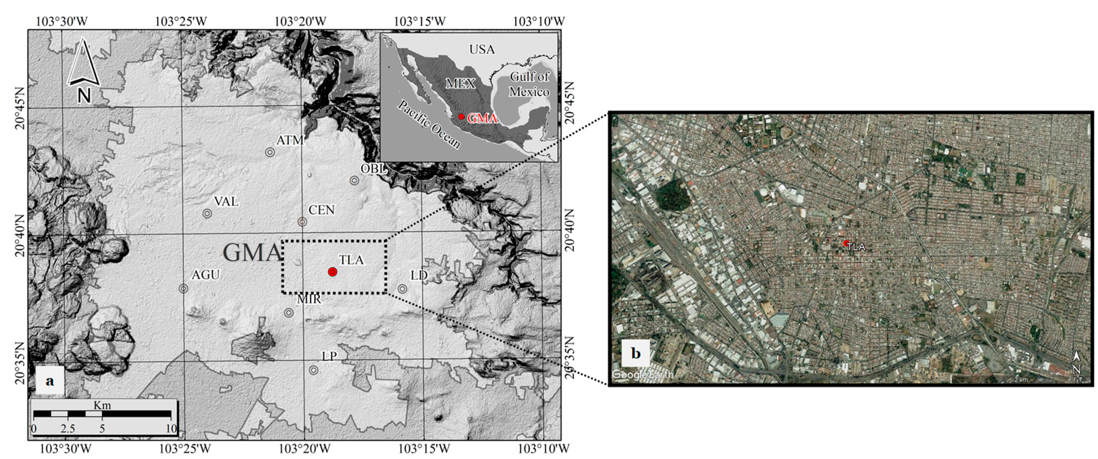
2.1. Study Area

The GMA is located some 550 km to the west of Mexico City. It has a population of around 5 million inhabitants [36], and a vehicle fleet of around 2.1 million vehicles that contribute with 80% and 70% of total oxides of nitrogen (NOX) and volatile organic compounds (VOCs) emissions within the GMA [37]. It is located in a semi-closed valley with prevailing calm winds and recurrent thermal inversions, approximately 283 days of the year [38]. Anti-cyclonic systems generated in the Gulf of Mexico and the Pacific Ocean may cause recurrently atmospheric stability and prevent vertical mixing. High photochemical activity is also observed during spring–summer due to its latitude 20° N [39]. Díaz-Torres et al. [40] estimated that the annual irradiation average at GMA is 5.69 kWh m−2 d−1 (variation range from 5.43 to 5.80 kWh m−2 d−1).

2.2. Sampling Site

Measurements of quinones and PAHs concentrations in the gas and PM1 phases were made at the Tlaquepaque monitoring site (TLA), which is part of the Air Quality Monitoring Network of the Jalisco State Government (SIMAJ). TLA is located on the roof of a public library building around 4 km NE of the GMA downtown (20°38′27” N, 103°18′45” W, 1622 m. a.s.l.), and is strongly influenced by vehicular emissions due to its proximity to the Niños Heroes and Revolucion roads (Figure 1). It is surrounded by several schools, restaurants, and large residential areas with medium and high population density (109–157 persons per hectare). Continuous measurements at a frequency of 1 h for O3, NO, NO2, NOx, SO2, and CO have been performed at TLA since 1996 by SIMAJ. The ambient air is sampled through an air inlet located 6 m above ground. Air pollutant measurements, calibration, maintenance procedures, and quality assurance/quality control (QA/QC) followed the protocols established in the Mexican standards NOM-036-SEMARNAT-1993 and NOM-156-SEMARNAT-2012.

2.3. PAHs and Quinones Sampling

Ambient air was sampled with low-volume speciation sampler Partisol Model 2300 (Rupprecht and Patashnick Co., New York, NY, USA) with four channels, which allows obtaining smaller breakthrough volumes and collects sufficient sample for analysis of semivolatile organic compounds SVOCs by combining the samples from 4 channels [41,42]. The sampling train (ChemComb 3500, Thermo Fisher Scientific Inc., Waltham, MA, USA) was integrated by an anodised inlet with a PM1 impactor, followed by a quartz filter (Ø 47 mm, Whatman) for PM1 collection. The quartz filters were pre-baked at 650 °C for 8 h to remove trace organic materials (by store or manufacturing). The gas phase was collected using 47 mm polyurethane foam (PUF, Thermo Fisher Scientific Inc., Waltham, MA, USA)/2 g of Amberlite® XAD-4 adsorbent material (Sigma-Aldrich Co., St. Louis, MO, USA)/PUF sandwich (PXP), which was cleaned before sampling with n-hexane and dichloromethane in a ratio 1:1 by sonication for two periods of 30 min.
The samples of the gas phase and PM1 were collected following the methodology reported by Tsapakis and Stephanou [20] which consists of a three-day intensive campaign with six sampling periods per day (07:00–11:00, 11:00–15:00, 15:00–19:00, 19:00–23:00, 23:00–03:00, 03:00–07:00 CDT, Central Daylight Time). The sampling scheme was performed during the warm-dry season (high temperature and solar radiation with clear skies conditions) on weekdays during 16–19 May 2016. Samplings were carried out at a flow rate of 16.7 L per minute (Lmin−1), following the recommendation of Ward and Smith [43], to increase sampling efficiency. Four samples of each phase were collected per period with a total collection of 72 samples of each phase (144 samples overall). In the laboratory, the samples were combined to obtain a more concentrated composite sample. In total, 18 composite samples were obtained for the gas phase analyses and 18 samples for the PM1 phase. The samples were stored at 4 °C during collection and then transported to the laboratory for storage at −20 °C until analysis.

2.4. Analytical Procedures

Prior to extraction, quartz filters and PXP were spiked with surrogates (SS) (Sigma-Aldrich) at 1600 ng mL−1 (fluorene-d10, fluoranthene-d10, pyrene-d10, benzo[a]pyrene-d10, 1,4-naphthoquinone-d6, anthraquinone-d8) to quantify the effect of the sample processing methodology on the analytes of interest. The extraction of PAHs and quinones from the gas and PM1 phases was performed using methylene chloride (25 mL for PM1 and 40 mL for the gas phase) of HPLC grade (Honeywell Burdick & Jackson Company, Muskegon, MI, USA) in an ultrasonic bath (Branson model 5800, Emerson Electronic Co., Wallingford, CT, USA) at 45 °C for 30 min [44,45]. This step was repeated twice, each one with a clean solvent (to improve the extraction efficiency), recovering the extractant in a flask. Then, the combined organic extract was concentrated up to obtain an approximate remaining volume of 1 mL by rotary evaporation (RV 10 digital. IKA®-Werke, Breisgau, Germany) at 120 rpm, 127 mmHg and 36 °C. The organic extract was filtered through a polytetrafluoroethylene (PTFE) membrane of 0.45 μm diameter (PALL Corporation, New York, NY, USA), and then evaporated to near dryness under a gentle stream of nitrogen (chromatographic grade, purity 99.998%) in a Six Port Mini-Vap (SUPELCO, Darmstadt, Germany). Then, the filtered extracts were resuspended with methylene chloride (90 μL) and, finally, five internal standards (IS) (Restek, PA, USA) (naphthalene-d8, acenaphthene-d10, phenanthrene-d10, chrysene-d12, perylene-d12) were added as proxies at a concentration of 1600 ng mL−1 (10 μL) in order to monitor the instrument signal.

2.5. Gas Chromatography–Mass Spectrometry (GC–MS)

The samples and standards were analysed in a gas chromatograph (GC) (6890N, Agilent Technologies Inc., Santa Clara, CA, USA), coupled to a mass spectrometer (MS) (7683B, Agilent Technologies Inc., Santa Clara, CA, USA). The injection of 1 μL per sample was performed automatically (Agilent Technologies 7683B) at 300 °C in split-less mode. For the identification of trace compounds, a capillary column CP-Sil 8 CB diphenyl dimethyl polysiloxane (Agilent J & W) of 30 m length, 0.25 mm internal diameter, and 0.25 μm film thickness, with high purity Helium as carrier gas (1 mL min−1), was used. The transfer line temperature was set at 310 °C to avoid condensation of the separated compounds. The mass spectrums were obtained using the electron impact (EI) mode (70 eV). The SCAN mode (40–400 uma) was used to optimise the instrumental method with standards, later the SIM mode to quantify the separated compounds (Retention times and SIM ions used in the analysis of PAHs and quinones is shown in detail in Table S1).
For sample separation, a temperature ramp was set starting at 40 °C and increased at a rate of 20 °C min−1 up to 110 °C, 5 °C min−1 up to 300 °C, and finally at 2 °C up to 310 °C for 10 min.

2.6. Quality Assurance/Quality Control (QA/QC)

Field blanks, laboratory blanks, and method blanks were carried out in order to monitor and control potential losses or sources of contamination during all steps. PAHs and quinones in all blank analysis were below detection limits, therefore, no blank correction was required because no sources of contamination were identified.
To ensure the accuracy and precision of the PAHs and quinones analysis process of this study, calibration curves were performed for a concentration range from 10 to 5000 ng mL−1 (R2 > 0.99) (surrogates and internal standards at 1600 ng mL−1). The limits of detection (LOD) were estimated from three times the standard deviation of the mean of lab blanks signals (Table S2). The method of internal standard was used to quantify PAHs and quinones, calculating response factors for each target analyte relative to one of the internal standards and obtaining the relative standard deviation of the response factor (Table S3). The recovery percentages of individual surrogates (SS) ranged from 83.5 ± 28% to 104 ± 16%.
Sixteen USEPA priority PAHs Mix were used as standards (Restek, PA, USA): naphthalene (Nap); acenaphthylene (Acy); acenaphthene (Ace); fluorene (Fl); phenanthrene (Phe); anthracene (Ant); fluoranthene (Flu); pyrene (Pyr); benzo[a]anthracene (BaA); chrysene (Chr); benzo[b]fluoranthene (BbF); benzo[k]fluoranthene (BkF); benzo[a]pyrene (BaP); dibenz[a,h]anthracene (Dib); benzo[g,h,i]perylene (BghiP) and indeno[1,2,3–c,d]pyrene (Ind). Also, eight individual quinones (Chiron AS, Trondheim, Norway): 1,4-naphthoquinone (1,4-NQ); 1,4-phenanthrenequinone (1,4-PQ); 9,10-anthraquinone (9,10-AQ); 1,4-anthraquinone (1,4-AQ); 9,10-phenanthrenequinone (9,10-PQ); 1,2-benzanthraquinone (1,2-BAQ); 1,4-chrysenequinone (1,4-CQ) and 5,12-naphthacenequinone (5,12-NAQ). However, only 14 PAHs and 7 quinones were present in the samples.

2.7. Meteorological Parameters

Ambient temperature (T), relative humidity (RH), dew point (DP), wind speed (WS), wind direction (WD), solar radiation (SR) and UV index (UV) were recorded at TLA every 10 min during the sampling period using a Davis Vantage Pro2 weather station (Davis Instruments, Davis, CA, USA).

2.8. Diagnostic Ratios

Diagnostic ratios allow the identification and assessment of multiple pollution sources in a particular monitoring site [46]. They are based on the assumption that PAH isomers have relative thermodynamic stability or similar physical and chemical properties and, therefore, will be transformed and degraded at the same rate, preserving the ratio that is present in the emission [47,48]. Four diagnostic ratios were selected from literature according to their estimated lifetime: Phe/(Phe+Ant), BaP/(BaP + Chr), BbF/BkF, and Ind/(Ind + BghiP).

2.9. Statistical Analysis

Statistical test and analysis were performed using Minitab 16 and OriginPro 2016 at a significance level of p < 0.05. Normal distributions of the data were analysed using the Shapiro–Wilk normality test, and since the data set were not normally distributed, a non-parametric tests analysed the difference between medians. The Mann–Whitney test was used for comparing two medians from different groups of data. The Spearman rank correlation was used to test relationships between quinones and PAHs with meteorological parameters (T, RH, DP, WS, SR, and UV index) and criteria pollutants (for O3, NO, NO2, NOx, SO2, and CO).

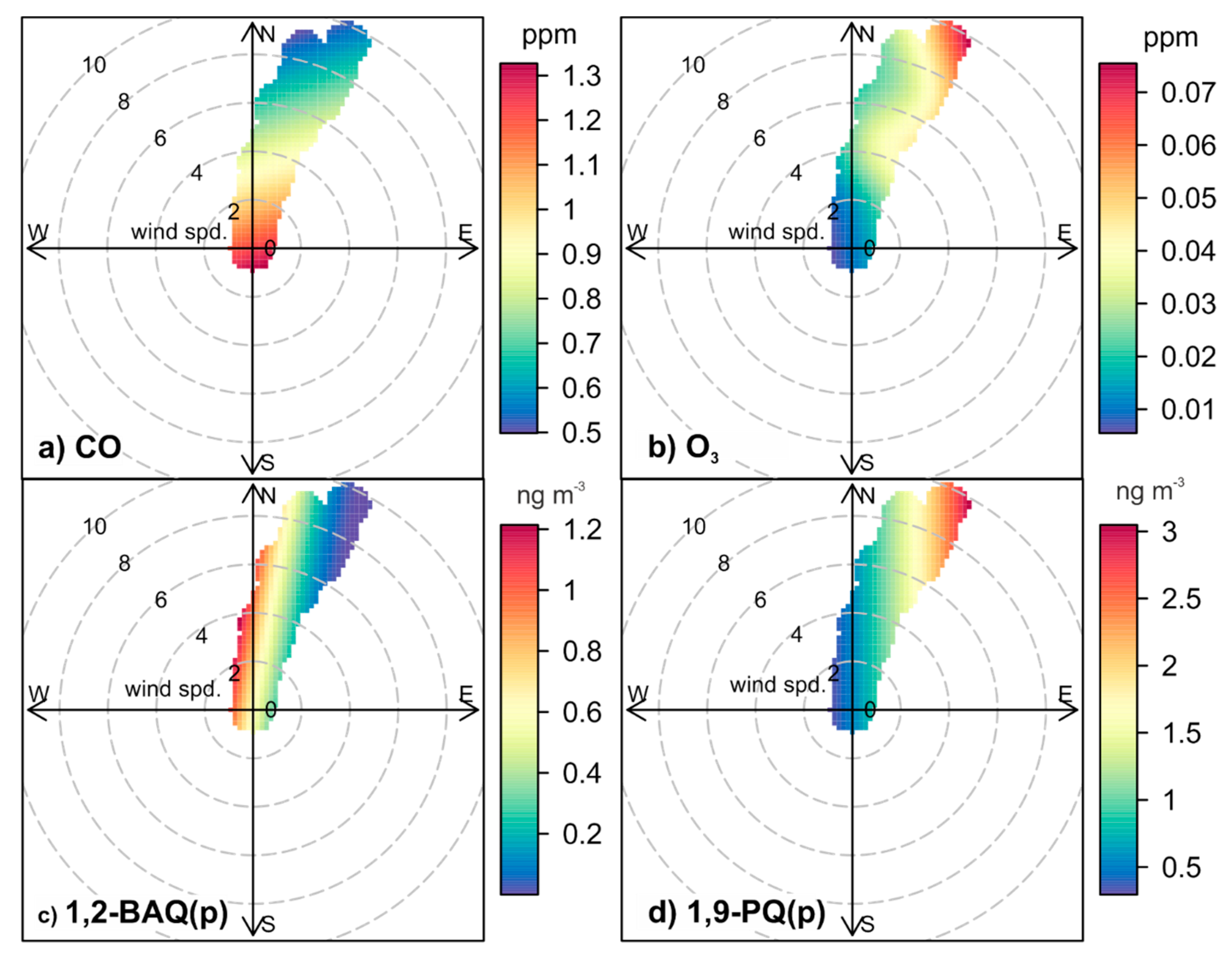
2.10. Polar Plot Analysis

Bivariate polar plots were constructed to show how the air pollutants vary with WD and WS at the TLA site [49,50]. However, other functions and variables can be used to help differentiate between source characteristics in some way due to different source types responding differently to values of the angular scale [51]. Bivariate polar plots were made using the openair-R package, and the methodology and use have been reported in detail elsewhere [50]. Briefly, in order to construct the bivariate plots, the time-series of air pollutants, meteorology, and quinones are aggregated into WS and WD bins (intervals) and then summarised using an aggregation function as the average or maximum. Then, the depicted continuous surface is obtained by fitting the smoothed surface to the defined binned summaries through a generalised additive model. Here, data of quinones concentrations, along with CO and O3 used as markers of primary and secondary sources, respectively, are addressed in order to suggest possibly the source of emissions along the air mass trajectories before arriving at TLA.

3. Results and Discussion

3.1. PAHs

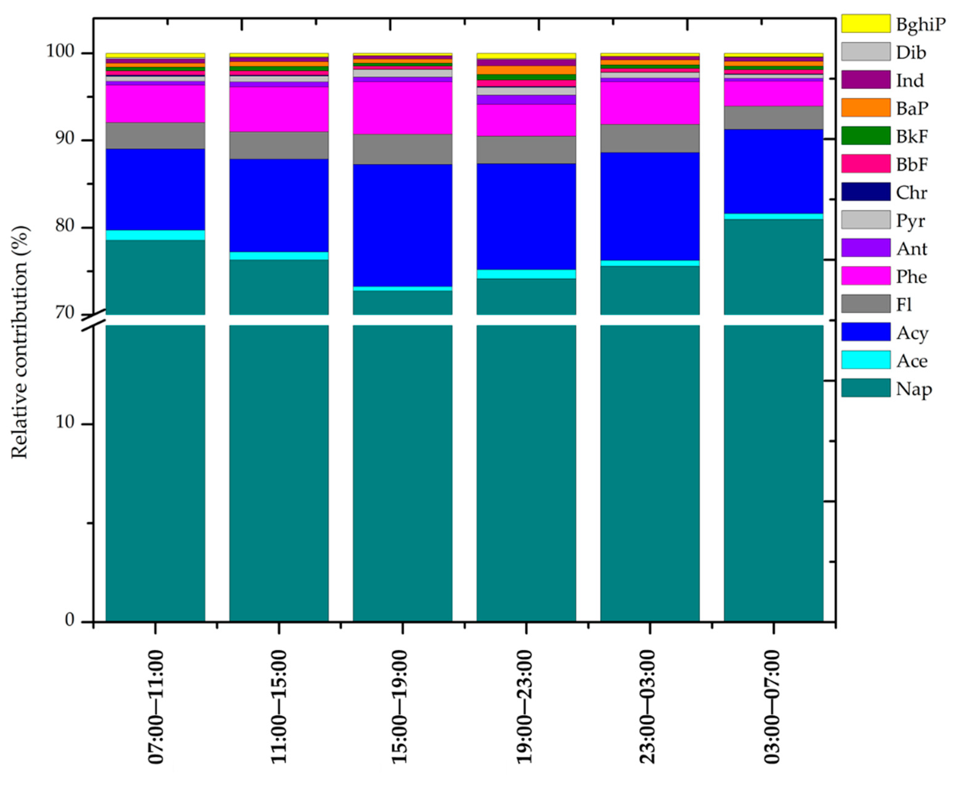
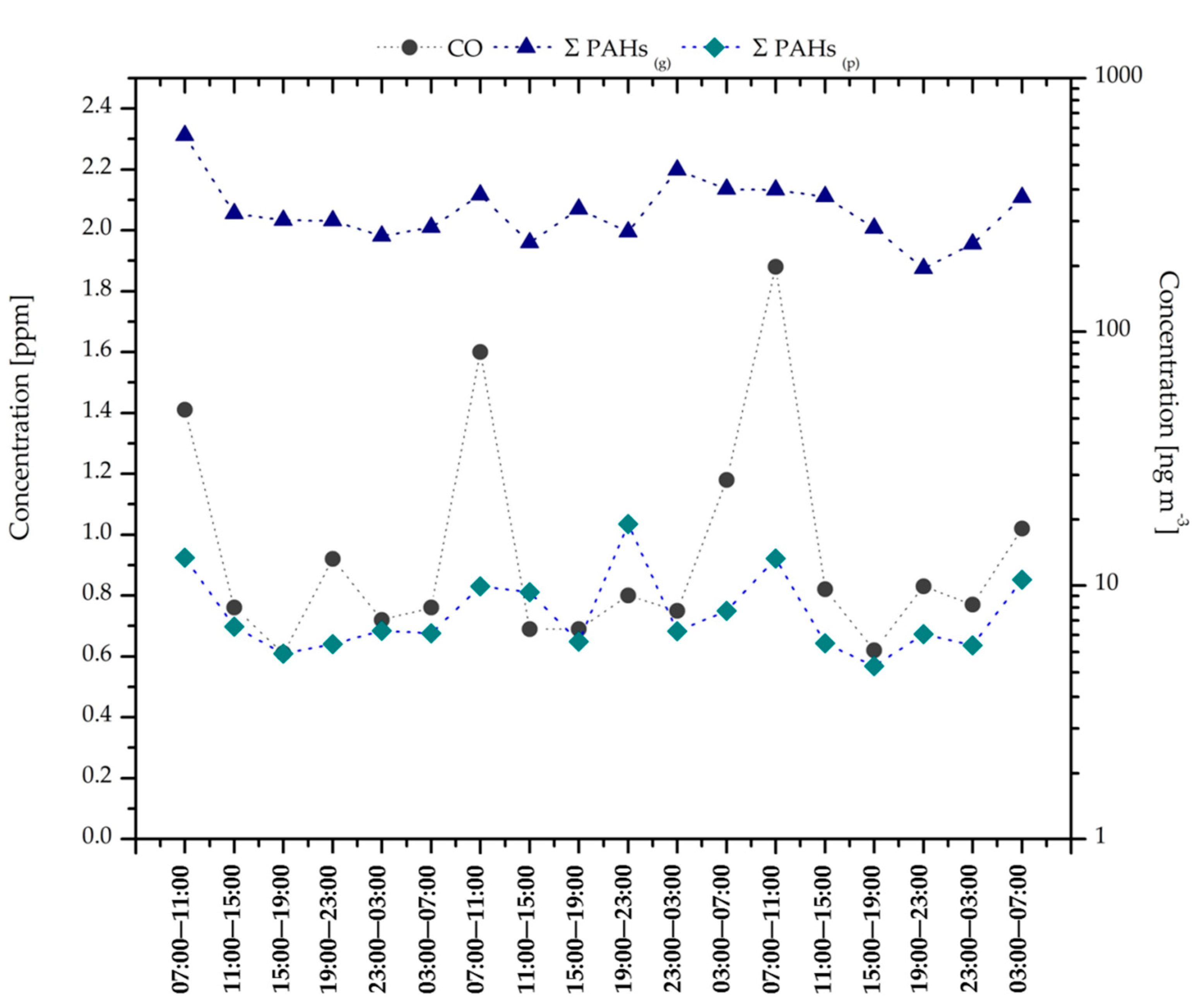
3.1.1. Ambient Levels and Distribution

Table 1 shows the average concentrations by sampling period of individual PAHs observed at TLA. Overall, fourteen PAHs were determined in both phases. In the gas phase, the ΣPAHs (the sum of concentrations for PAHs in the gas or PM1 phase) ranged from 177.6 (18 May, 19:00–23:00 h) to 595.0 (16 May, 07:00–11:00 h) ng m−3, while in the PM1 ranged from 4.81 (18 May, 15:00–19:00 h) to 17.4 (17 May, 19:00–23:00 h) ng m−3. The highest average (between same periods) concentration of ΣPAHs(gas) was observed during morning time at 07:00–11:00 h (434.4 ± 139.3 ng m−3), followed by the period at 03:00–07:00 h (320.9 ± 55.99 ng m−3). Morville et al. [52] observed a higher concentration of PAHs gas during periods of greater vehicular flow in urban and suburban sites in Strasbourg, France. In the TLA area, public transport and vehicle activity start at 05:00 h due to the distances people must travel to reach schools and workplaces. Therefore, this suggests that the measured PAHs are likely due to motor vehicle emissions. No significant differences (p > 0.05) were observed among concentrations recorded for the other periods, possibly due to similar vehicular activity during the rest of the day. Figure S1 shows the daytime/nighttime ratios for the individual PAHs. The average ΣPAHs during the daytime were 1.21 and 1.04 times higher than the night values in the gas and particle phases respectively. The highest daytime/nighttime ratio in the gas phase and PM1 were observed for Chr and Dib.
For the gas phase, the levels of PAHs reported at the TLA site are similar to those observed in Crete, Greece, by Tsapakis and Stephanou [20], when sampling during three days in periods of 4 h (Fl 4.2 ng m−3, Phe 22.9 ng m−3, Ant 3.0 ng m−3, and Pyr 1.6 ng m−3). While for PAHs in particles within the GMA are an order of magnitude higher than in Greece (total suspended particles, TSP, sampled in Crete), a lower population in Crete with lower emissions of particles could explain the observed differences. In contrast, the levels for Nap (244.5 ng m−3) and Phe (13.7 ng m−3) within the GMA are similar to those of 217.5 ng m−3 and 10.1 ng m−3, respectively, reported by Reisen and Arey [30] for Los Angeles, California, when sampled during summer at intervals of 03:30 h. Likely, the observed similar levels for PAHs in the GMA and Los Angeles arise from a similar number of inhabitants with high vehicular activity in both cities. Nevertheless, compared to the GMA, higher levels of ΣPAHHMW (sum of PAHs of 4, 5, and 6 rings) bound to PM1 were reported for Kanpur, India, of 373.97 ng m−3 when sampled during foggy days over winter [53]. A possible explanation for the observed differences was that winter inversions in Kanpur, India, related to atmospheric stability that prevented emissions dispersion.
The results of our previous study [44] carried out in April–June 2015 during sampling periods of 24 h in TLA obtained an average of Σ16PAH in the gas phase of 137 ± 37.7 ng m−3 and Σ16PAH in PM1 of 7.25 ± 8.34 ng m−3. Comparing each 4 h period in this study was 1.7 to 3.17 times higher in the gas phase and 0.74 to 1.63 times higher in PM1. Reisen and Arey [30] report PAHs and nitro-PAHs in periods of 3.5 h in Los Angeles, California. The values of Nap (which is the most abundant PAH) were reported for August 2002 in the range of 127–389 ng m−3 in the gas phase, while Eiguren-Fernandez et al. [54] reported an average of Nap in 24 h sampling (July 2002–November 2003) of 389 ng m−3 (also in the gas phase). Each period of 3.5 h is up to 2.6 times higher than the value reported for 24 h. Such differences may arise from sampling artefacts such as volatilisation and chemical processing (times of reaction under high temperature and UV radiation) [55]. It has been reported that SVOCs and PAHs, in particular, may significantly degrade in the gas phase due to reactions with OH and O3, whereas those in PM can be underestimated due to reactions with reactive compounds (e.g., benzo[a]pyrene) [56]. In this study, only Nap, Ace, Acy, Fl, Phe, Ant, Pyr, and Chr were observed in the gas phase, while only Pyr, Chr, BbF, BkF, BaP, Ind, Dib, and BghiP were observed in PM1. Lee et al. [57]suggested that absence of low molecular weight (LMW, <228 Da) PAHs in particles and the presence of high molecular weight (HMW, <228 Da) PAHs in the gas phase in the sorbent material (PXP) suggests a reliable sampling, as observed in this study.
Figure 2 shows the average relative contribution per sampling period (24 samples per period) of each PAH to the total PAHs (PAH / Σ14PAH) in both phases expressed as a percentage. Overall, the most abundant PAHs corresponded to LMW species, with the major contribution observed for Nap (>70%), while the HMW contribution compounds were <3% (mainly associated to the PM1 phase). This is consistent with the results of Ho et al. [58] from Hong Kong, who observed during summer a contribution for gas–particle phases of 97% for LMW and 3% for HMW in a vehicle tunnel with a volume of ~53,000 vehicles per day. Although the most abundant PAHs observed in Hong Kong were Ace (47%), Nap (21%), and Acy (17%), the similar contributions suggest that vehicle emissions notably influence the PAHs concentrations within the GMA. Different relative contributions estimated for particle and gas phases in the whole samples suggest that the population within the GMA is moderately exposed to carcinogenic PAHs.
Figure 3 shows the average distribution of PAHs in ambient air according to their vapour pressures (p °L) (ranging from 38 Pa for Nap to 9.5 × 10⁻⁸ Pa for Dib at 298 K). Vapour pressures for other PAHs have been reported in Keyte et al. [28], and are the following: 1 × 101 (Nap); 1 × 100 (Ace, Acy); 1 × 10⁻¹ (Fl, Phe); 1 × 10⁻² (Ant); 1 × 10⁻³ (Pyr); 1 × 10⁻⁴ (Chr); 1 × 10⁻⁵ (BbF); 1 × 10⁻⁶ (BkF, BaP); 1 × 10⁻⁷ (Ind, BghiP) and 1 × 10⁻⁸ (Dib). It can be noticed that the PAHs concentration increases with the vapour pressure mainly in the gas phase, while in PM1, the largest distribution of PAHs lies between 1 × 10⁻⁵ and 1 × 10⁻⁷ Pa. A negative correlation (p < 0.05) between compounds with 1 × 10⁻⁵ and 1 × 10⁻⁷ Pa and temperature was observed, likely due to the influence of evaporation by a relatively high ambient temperature typical within the GMA most of the year [59]. This phenomenon has been reported previously in an urban region of Greece by Tsapakis and Stephanou [60], where temperature changes typically from day to night around 10 °C, despite seasonal variations.

3.1.2. PAH Diagnostic Ratios

In order to provide further insights into the origin of PAHs, average diagnostic ratios were calculated by sampling period and are listed in Table 2. The reference values for source identification were obtained from the study made by Slezakova et al. [61] in Oporto, Portugal, for gas and particles at low-flow sampling. For the calculation of diagnostic ratios, PAHs concentrations in both phases were considered according to the methodology of Tobiszewski and Namieśnik [46]. It is important to mention that the methodology used only considers one diagnostic ratio applicable to the gas phase since the rest of the PAHs are mainly sorbed in PM. Other limitations of the method have been documented, mainly due to the physical and chemical characteristics of PAHs, oxidant species, and solar radiation, which can modify the fingerprint of the sample by altering the results of the true source [62]. However, these uncertainties could decrease with short sampling periods and decreasing distances to the source. Thus, these results could be used to compare this method with other subsequent studies.
The Phe/(Phe + Ant) indicator showed an overall average of 0.88, suggesting a strong influence of motor vehicle emissions for the gas phase in all sampling periods. Similarly, the BaP/(BaP + Chr) indicator exhibited a value of 0.87, which is likely to correspond to the combustion of gasoline [46].
Consistently, the BbF/BkF and Ind/(Ind + BghiP) indicators showed average values of 1.09 and 0.53, respectively, suggesting enhanced emissions of diesel-powered engines at the TLA site. In urban environments, diesel exhaust particles may represent up to 90% of total submicron particles, and since we observed that BbF, BkF, Ind, and BghiP were sorbed mostly in PM1 [63], this suggests a primary origin for the PAHs observed at TLA. Similar abundant levels of Nap and Acy in Los Angeles and Riverside, California [30], have been related to predominant emissions from cars and light vehicles [64,65], and emission of diesel vehicles [66].

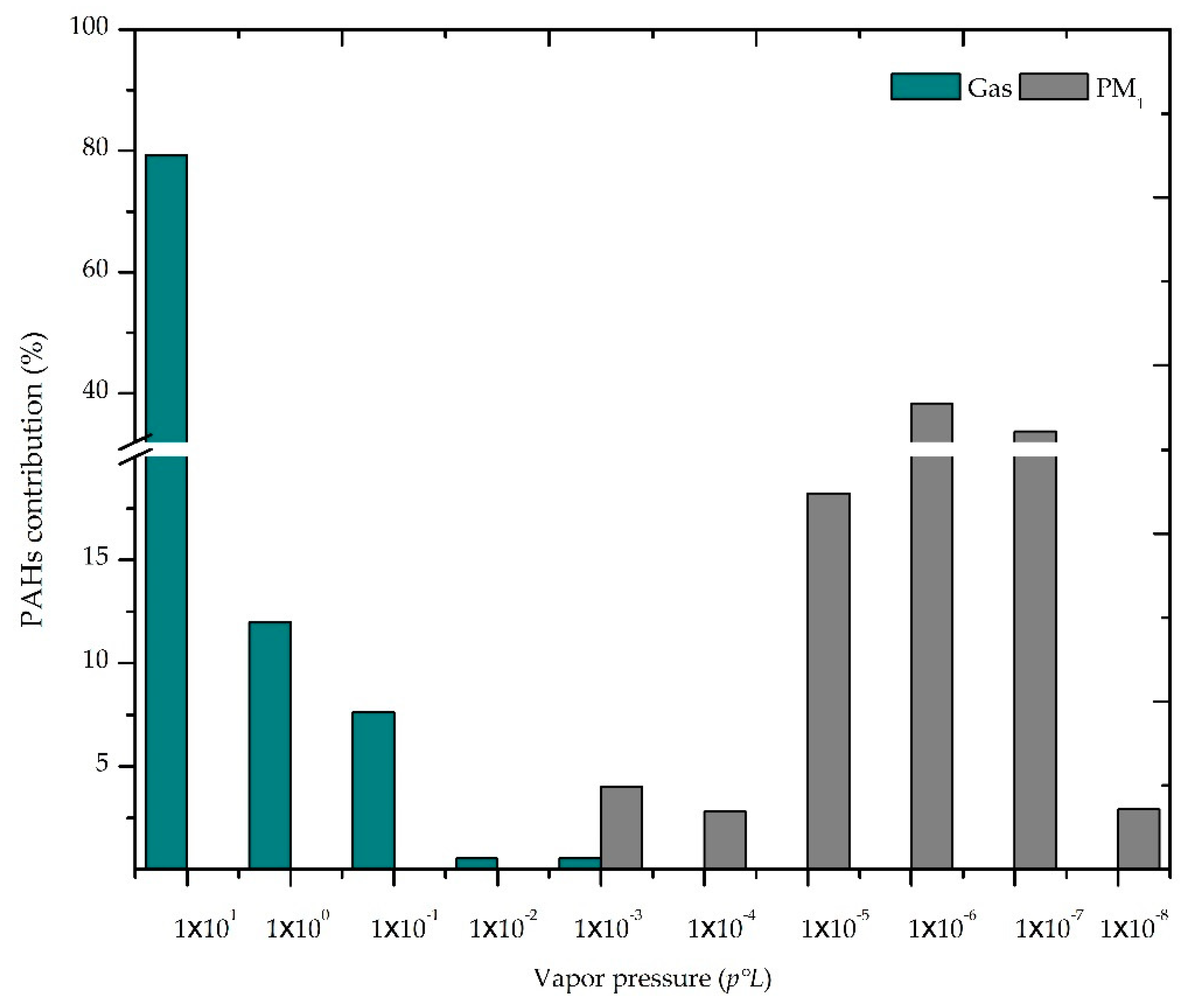
3.1.3. PAHs and Influence of Primary Emissions
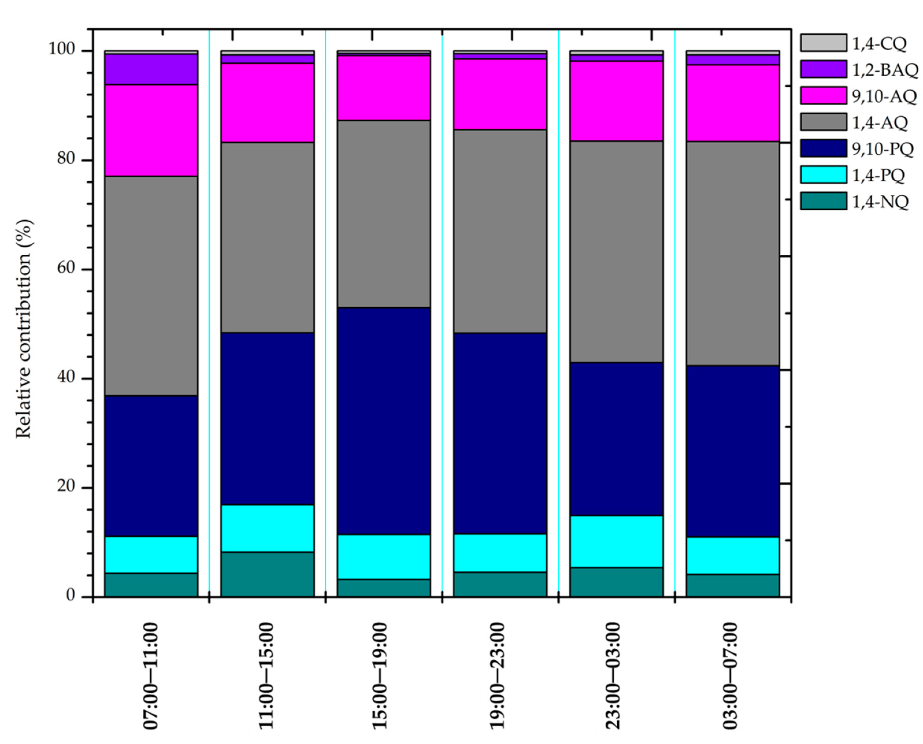
Figure 4 shows the sum of total PAHs in the gas and PM1 phases and CO ambient concentrations. The Spearman’s rank analysis shows that PAHs have a strong correlation with CO and NO of 0.71 to 0.88, respectively (p < 0.05), confirming significant PAHs emissions from local sources [35]. Besides, PAHs both in the gas and PM1 phases showed a negative correlation with temperature (0.73 and 0.81, respectively) and a positive correlation with RH (0.68 and 0.83, respectively) (p < 0.05). This is in agreement with the report of Gu et al. [67] for diurnal variations of PAHs in an urban site in Shanghai, China, where significant correlations between PAHs and temperature suggested the degradation and volatilisation of LMW-PAHs associated in the gas phase [68], and an increase in evaporation of HMW-PAHs from particles [20]; whereas, increases in humidity could lead to the partition gas/particle [69]. Correlation analyses between PAHs and marker compounds from combustion emissions were carried out to identify potential emission sources. The individual PAHs such as Nap, Ace, BbF, and BghiP showed positive correlations with NOX (0.75–0.82; p < 0.05), while Nap, Acy, Ant, BbF, BbK, Ind, Dib, and BghiP showed correlations with CO (0.68–0.84; p < 0.05). These correlations may indicate that they are primarily emitted from local sources and may also be associated with regional-scale emissions [35].

3.2. Quinones

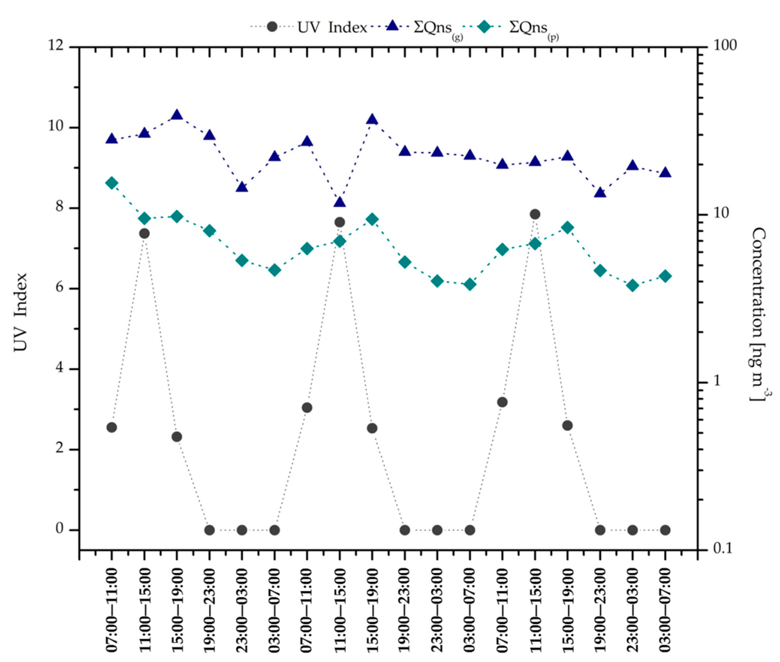
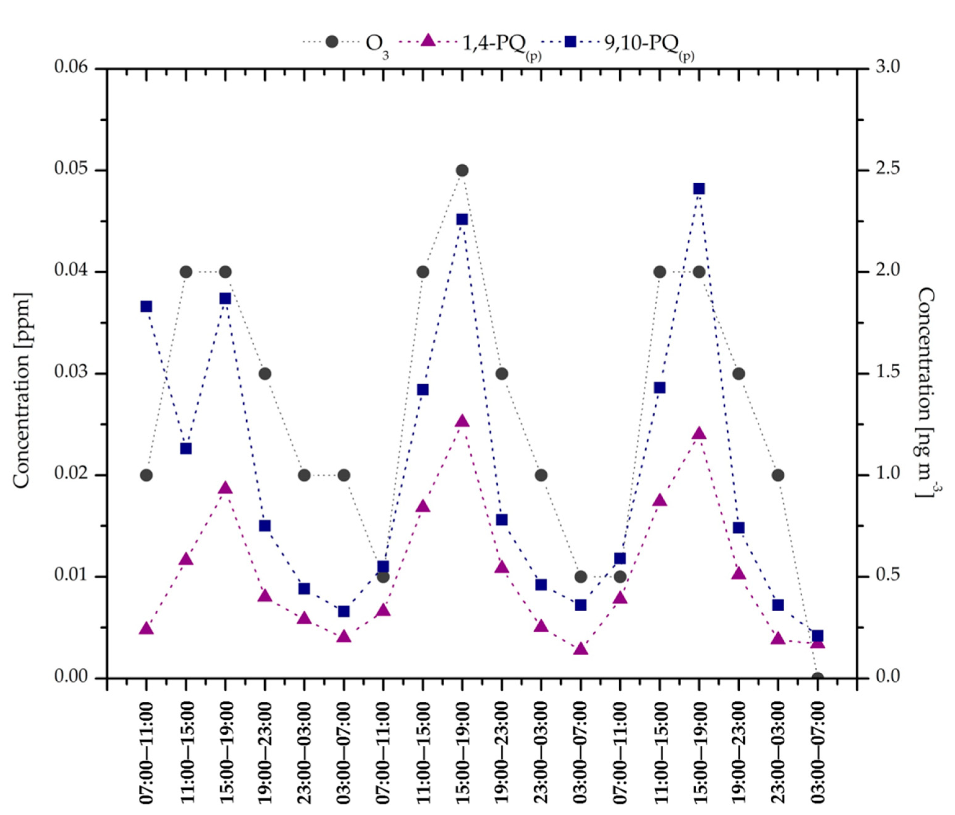
3.2.1. Ambient Levels and Distribution

Overall, seven quinones were identified in the samples collected (gas + PM1). The total concentration of quinones (Σ7Quinones) for periods of 4 h ranged from 18.0 (19:00–23:00 h) to 48.8 (15:00–19:00 h) ng m−3, with an average of 30.2 ± 9.40 ng m−3. Table 3 shows the quinones average concentrations observed at TLA by the sampling period. The quinones daily cycle shows the trough during nighttime and the peak by 15:00–19:00 h. Peaks of nitro-PAHs have been observed by midday (11:00–15:00 local time) at Crete, Greece, ascribed to high photochemical activity [20]. It also has been reported that increases in quinones concentrations during daytime is influenced by vehicle activity in combination with high temperature and SR [4]. Figure S2 shows the daytime/nighttime ratios for quinones. The average ΣQuinones during the daytime were 1.26 and 1.77 times higher than the nighttime in the gas phase and PM1, respectively. The highest daytime/nighttime ratios were determined in PM1 for 9,10-PQ (3.39) and 1,2-BAQ (3.08), probably due to the influence of solar radiation and vehicular traffic.
The average relative contribution of individual quinones to the ΣQns (Total) (gas + PM1) by sampling period shows the dominance of 9,10-PQ and 1,4-AQ (65–75%) (Figure 5). The 9,10-PQ is among the most-studied quinones because its emissions typically correspond with diesel exhaust particles [70], and it has been associated positively with the development of reactive oxygen species (ROS) and negative impacts to human health such as lung cancer, asthma, and allergic inflammation [5,71,72]. It was the most abundant quinone in the gas phase (9.0 ± 4.8 ng m−3), followed by the 1,4-AQ (7.4 ± 2.0 ng m−3), whereas the 1,4-AQ predominated (4.0 ± 0.90 ng m−3) in PM1. The concentrations found under this sampling scheme are between 2.5 and 4.5 times higher than those previously reported (2015) at TLA using sampling periods of 24 h [44]. These measurements can be explained by the decrease in positive and negative sampling artefacts. Consistently, Wnorowski and Charland [73] reported levels of quinones at the Athabasca oil sands region in Canada for 24 h periods lower than for 12 h periods. Nevertheless, the levels of quinones in the gas phase and TSP in this study are much higher than those reported by Wnorowski and Charland [73] of 1,4-NQ (0.059 ng m−3, 0.16 ng m−3), 9,10-PQ (0.049 ng m−3, 0.020 ng m−3), 1,4-AQ (0.065 ng m−3, 0.17 ng m−3), and 1,2-BAQ (0.028 ng m−3, 0.14 ng m−3), possibly due to different anthropogenic sources at both sites.
Figure 6 shows the contribution of quinones by their vapour pressure (p °L), which ranged from 0.10 Pa to 5.5 × 10⁻⁸ Pa at 298 K, as follows 1 × 10⁻¹ (1,4-NQ); 1 × 10⁻³ (9,10-PQ); 1 × 10⁻⁴ (1,4-PQ, 1,4-AQ, 9,10-AQ); 1 × 10⁻⁷ (1,2-BAQ, 5,12-NAQ); and 1 × 10⁻⁸ (1,4-CQ). The major contribution was observed for quinones with a vapour pressure of 1 × 10⁻⁴, which ranged from 57% to 67% in the gas phase and PM1, respectively. The compounds with intermediate vapour pressures were observed in both phases since their occurrence depends mostly on the ambient temperature [74,75].
In this study, 100% of the 1,2-BAQ and 1,4-CQ concentrations were observed in the particulate phase, while lower contributions were observed for 1,4-NQ (35%), 1,4-PQ (20%), 9,10-PQ (10%), 1,4-AQ (40%), and 9,10-AQ (2%). Such distribution is in good agreement with the report of Harrison et al. [74] for the 9,10-AQ (3.9%), 9,10-PQ (5.7%), and 1,2-BAQ (100%) quinones made on the coast of Saudi Arabia, north of Jeddah, near to major roads and with a population of 5 million, with peak temperatures of 47 °C in summer. From the overall distribution, the gas phase accounts for 79% of the observed quinones, which is consistent with the results reported by Jakober et al. [76], who found 69% and 84% of gas-phase quinones from gasoline and diesel emissions from motor vehicles, respectively. These results may indicate that these gas-phase quinones are direct emissions from incomplete combustion of fossil fuels.

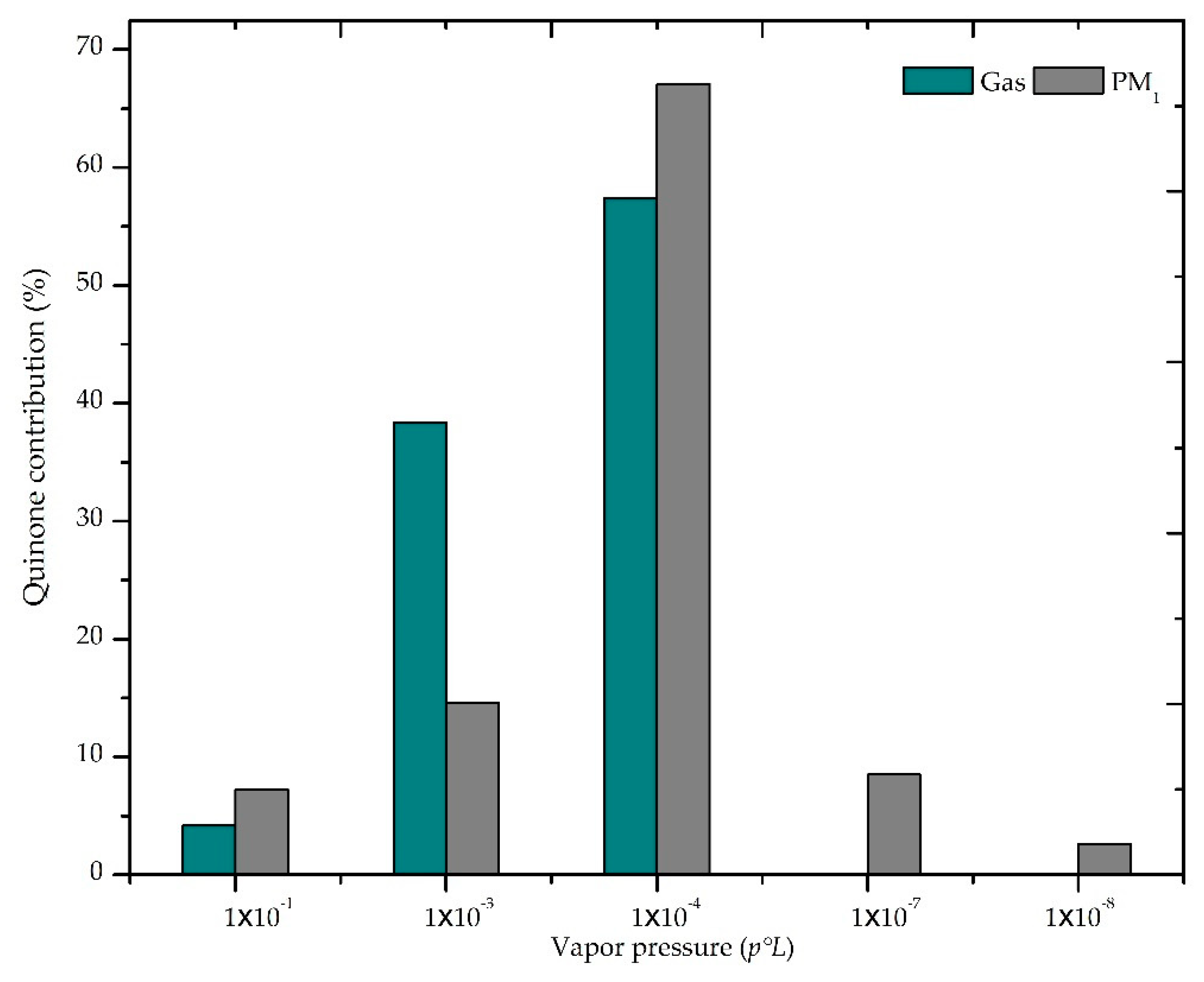
3.2.2. Possible Sources

Figure 7 shows the sum of quinones in the gas and PM1 phases and the UV index, with significant correlation (p < 0.05) between PM1 and UV index, r = 0.63. This behaviour suggests that the increase of quinones in PM1 can be via photochemical pathways. After light absorption, PAHs are excited to their upper energy states that can initiate a series of excited-state reactions leading to other intermediates such as quinones [77,78]. During the daytime, the 1,4-NQ in the gas phase shows a positive association with CO (0.80) and NOx (0.85) (p < 0.05). This relation over urban areas essentially represents combustion-related emissions [79]. The 1,4-NQ in PM1 through nighttime showed negative correlations with RH and DP (−0.72, −0.92, respectively), which may indicate a process of suppression in the adsorption of SVOCs in the gas phase into particles [80]. Particles formation and condensation of SVOCs processes are highly favourable during conditions of low temperature and high RH [81].
On the other hand, during nighttime, the 1,4-PQ in the gas phase showed correlation (p < 0.05) with Phe (0.95) and NOx (−0.69), indicating that NOx could react with their congener PAH (Phe) [72]. It has been reported that Phe has an average lifetime of 4.6 h, which makes it very reactive [82]. Although, during the daytime, the 1,4-PQ showed significant correlations with Acy (0.91) and 9,10-PQ(g) (0.81), suggesting that both could share a common emission source [83]. In contrast, the negative correlation with UV (−0.93) suggests degradation to other products during the same period of the day. The 9,10-PQ(g) showed correlations only with Acy (0.78) and UV (−0.66), which is similar to the diurnal behaviour of their isomer. Additionally, the 1,4-PQ and 9,10-PQ have been reported in the gas phase, involving their precursors with species such as O3, OH, and NO3 [84], or as primary emissions due to incomplete combustion of fossil fuels, particularly diesel [85]. The observations of this sampling scheme have shown that the atmosphere of the GMA has geographic-meteorological (high UV radiation and high temperatures) characteristics that have a strong influence on the levels of some PAHs and quinones of study.
When the concentrations of quinones in PM1 was tested for correlations, the 1,4-PQ(p) (r = 0.97) and 9,10-PQ(p) (r = 0.83) showed positive correlations (p < 0.05) with temperature, UV (0.56, 0.60, respectively), and WS (0.86, 0.82, respectively), while negative correlations were determined with CO (−0.79, −0.75, respectively), NO2 (−0.73, −0.58, respectively), and RH (−0.91, −0.76, respectively). Additionally, Figure 8 shows trends of 1,4-PQ(p) and 9,10-PQ(p) in PM1 with respect to primary and secondary pollutants and their peaks in different periods of the day. These results suggest that the major source of such quinones is secondary production, as these can be formed through photochemical processing during daytime under UV radiation and the presence of OH [72,86]. In contrast, during nighttime, the phenanthrenequinones are mainly products of reactions with nitrate radicals that proceed from reactions involving NO2 and O3 [87]. The influence of WS suggests that the secondary transformation also may occur during the transport of air masses [16], as reported for the 90% formation of 9,10-PQ during transport in Los Angeles, California [88].
The 1,4-AQ has been documented in particulate matter from motor vehicle emissions but not as a product of its Ant precursor degradation [89,90]. In marked contrast, the 9,10-AQ did show significant correlations with temperature (0.86), NO2 (−0.84), O3 (0.84), RH (−0.79), and WS (0.89), highlighting the influence of secondary formation upon the 1,4-AQ levels observed within the GMA. In particular, the 9,10-AQ has been reported as a product of O3 reaction with Ant [89], and as derivative from the NO3 radical (which involves the competition of NO2 with O3) during nighttime [91]. The 1,2-BAQ showed positive correlations with NO (0.76) and CO (−0.74), confirming the influence of motor vehicle contributions for other quinones [92]. The 1,2-BAQ has been reported as a compound highly resistant to photodecomposition, with an average lifetime of 34.9 h, which gives greater reliability to the correlations obtained in this study [78].

3.2.3. Cluster Analysis

Primary emissions and secondary production of quinones were analysed using relationships between quinones and air pollutants, and those with WS and WD. Meteorology recorded at TLA during the sampling scheme was used to produce daily averaged polar plots for CO, O3, 1,2-BAQ(p), and 9,10-PQ(p). During the sampling scheme, wind occurrence was predominantly from the north–northeast at WS, ranging between 0.1 and 10 km h−1. Figure 9 shows clear different patterns between the selected quinones and their relation with primary and secondary markers (CO and O3, respectively) with evidence of increasing concentrations for O3 and 9,10-PQ in particles when the WS increases from the north and northeast (Figure 9b,d). This may suggest that 9,10-PQ(p) and O3 observed at TLA are likely produced during the advection of air masses. In contrast, the highest concentrations of CO and 1,2-BAQ(p) are observed during lower WS, suggesting that primary sources can emit these because at high WS they decrease notably (Figure 9a,c).
Eiguren-Fernandez et al. [15,88] reported a contribution for the 9,10-PQ (in PM2.5) of diesel from the secondary formation at downwind monitoring sites in the Los Angeles metropolitan area, while primary emissions were observed to dominate the concentrations of those near the monitoring sites. This is in good agreement with our observations at TLA, where the highest concentrations are recorded for primary pollutants. Furthermore, the CO and 1,2-BAQ(p) levels are correlated (r = 0.70, p < 0.05), which suggests a common source, likely motor vehicles. However, some quinones detected at TLA are also derivatives from PAHs vehicular emissions but can be only observed in photochemically aged air masses, which explains the higher concentrations of O3 observed at high WS. This is because the parent PAHs of some secondary quinones measured at TLA are transformed during the transport of local emissions downwind within the GMA. Nevertheless, additional measurements over longer periods at monitoring sites of the SIMAJ network should be conducted in order to complement the understanding of secondary quinones production and other secondary toxic compounds within the GMA. This may help to design more effective air quality policies that reduce the levels of toxic air pollutants such as secondary quinones.

3.3. Limitations

We identified some limitations in the sampling scheme presented in this study, which are described as follows. Firstly, the data collected and samples representativeness are limited to the three days of sampling and may only be valid for the region where the study was conducted. A subsequent study should consider samplings at a larger number of sites spread over the GMA, during the summer and winter seasons in order to compare the effects of meteorological conditions on the photochemical processing of PAHs. An increase in the number of samples collected would help to obtain more robust statistical information and to establish more reliable conclusions. Also, the collection of data during two seasons would allow observing temporal changes in PAHs and quinones and possibly identifying transport within the GMA airshed. Finally, the availability of traffic counts could be used to constrain motor vehicle contributions to the ambient levels of PAHs and quinones, together with pollutant markers of traffic activity.

4. Conclusions

In this study, we presented new information about the distribution, diurnal variation, and origin of fourteen PAHs and seven quinones in the gas phase and PM1 during short-time lapses of sampling in one urban site in the GMA. The ΣPAHs and individual PAH levels varied throughout the day, and some of them showed positive correlations with some primary pollutants, like ΣPAHs(Total) versus CO and ΣPAHs(Total) versus NO (r = 0.71 and r = 0.88, respectively p < 0.05), suggesting that, at the TLA site, diesel and gasoline traffic emissions drive the ambient levels of PAHs. Meanwhile, the levels of quinones were higher during the daytime, suggesting the influence of vehicular emissions in some cases (i.e., 1,4-NQ in the gas phase versus CO and versus NOx, whit r = 0.80 and r = 0.85, respectively, p < 0.05), but also from meteorology variables (temperature, RH, and WS). An analysis of phase distribution indicated that PAHs and quinones are systematically distributed according to their vapour pressure (p °L) and molecular weight in the gas phase (Nap, Ace, Acy, Fl, Phe, Ant, Pyr, and Chr) and PM1 (Pyr, Chr, BbF, BkF, BaP, Ind, Dib, and BghiP). Correlation analyses showed that quinones in the gas phase were from primary sources, while the majority of quinones in PM1 proceeded from secondary transformation (e.g., 9,10-AQ versus O3, r = 0.84).
The sampling scheme used in this study allowed to obtain higher concentrations than in the previous sampling of PAHs and quinones in the gas phase and PM1. It is probable that, during 4 h sampling, the formation of artefacts be reduced compared with 24 h sampling, preventing the loss of significant information about their concentrations in the ambient air, and about source emissions. The results of PAHs and quinones (gas phase and PM1) from 4 h sampling offer more reliable information. Although the present study included a limited number of samples about the measurements of PAHs and qui3ones in two phases, this is not enough to represent the seasonal or annual variation cycle. The data from this campaign could be the basis for a more precise estimation of risk to human health at the sampling site by exposure to PAHs and quinones from the ambient aerosol. Finally, further measurements must be conducted to assess the role of quinones secondary production within the GMA.

Supplementary Materials

The following are available online at https://www.mdpi.com/2071-1050/11/22/6345/s1, Table S1: Retention times and SIM ions used in the analysis of PAHs and quinones by Gas Chromatography-Mass Spectrometry (GC-MS), Table S2: Linearity, limits of detection and sensitivity from PAHs and quinones standard solutions, Table S3: Surrogate (SS) and target compounds grouped under the internal standard (IS) compounds, Figure S1: Daytime to nighttime ratios for ambient levels of PAHs during the three days of sampling observed at the TLA site, Figure S2: Daytime to nighttime ratios for ambient levels of quinones during the three days of sampling observed at the TLA site.

Author Contributions

Conceptualization, L.H.-M. and A.L.-L.; data curation, J.d.J.D.-T.; writing—original draft preparation, V.O.-C.; dataset validation, writing—review and editing, I.Y.H.-P.; project administration, S.A.-R. and J.d.R.-O.; funding acquisition, S.A.-R. and J.d.R.-O.

Funding

This research was funded by SENER, grant number 234633 and SEP-CONACYT, grant number 183444.

Acknowledgments

We dedicate this paper to the memory of Alberto López-López who contributed to the conception and design of this study.

Conflicts of Interest

The authors declare no conflict of interest.

References

  1. Rengarajan, T.; Rajendran, P.; Nandakumar, N.; Lokeshkumar, B.; Rajendran, P.; Nishigaki, I. Exposure to polycyclic aromatic hydrocarbons with special focus on cancer. Asian Pac. J. Trop. Biomed. 2015, 5, 182–189. [Google Scholar] [CrossRef]
  2. Di Filippo, P.; Pomata, D.; Riccardi, C.; Buiarelli, F.; Gallo, V. Oxygenated polycyclic aromatic hydrocarbons in size-segregated urban aerosol. J. Aerosol Sci. 2015, 87, 126–134. [Google Scholar] [CrossRef]
  3. Nalin, F.; Golly, B.; Besombes, J.L.; Pelletier, C.; Aujay-Plouzeau, R.; Verlhac, S.; Dermigny, A.; Fievet, A.; Karoski, N.; Dubois, P.; et al. Fast oxidation processes from emission to ambient air introduction of aerosol emitted by residential log wood stoves. Atmos. Environ. 2016, 143, 15–26. [Google Scholar] [CrossRef]
  4. Wnorowski, A. Characterization of the ambient air content of parent polycyclic aromatic hydrocarbons in the Fort McKay region (Canada). Chemosphere 2017, 174, 371–379. [Google Scholar] [CrossRef] [PubMed]
  5. Shang, Y.; Zhang, L.; Jiang, Y.; Li, Y.; Lu, P. Airborne quinones induce cytotoxicity and DNA damage in human lung epithelial A549 cells: The role of reactive oxygen species. Chemosphere 2014, 100, 42–49. [Google Scholar] [CrossRef] [PubMed]
  6. Xia, T.; Korge, P.; Weiss, J.N.; Li, N.; Venkatesen, M.I.; Sioutas, C.; Nel, A. Quinones and aromatic chemical compounds in particulate matter induce mitochondrial dysfunction: Implications for ultrafine particle toxicity. Environ. Health Perspect. 2004, 112, 1347–1358. [Google Scholar] [CrossRef] [PubMed]
  7. Baek, S.O.; Goldstone, M.E.; Lester, J.N.; Perry, R. Phase distribution and particle size dependency of polycyclic aromatic in the urban atmosphere. Chemosphere 1991, 22, 503–520. [Google Scholar] [CrossRef]
  8. Chen, G.; Li, S.; Zhang, Y.; Zhang, W.; Li, D.; Wei, X.; He, Y.; Bell, M.L.; Williams, G.; Marks, G.B.; et al. Articles Effects of ambient PM1 air pollution on daily emergency hospital visits in China: An epidemiological study. Lancet Planet. Health 2014, 1, e221–e229. [Google Scholar] [CrossRef]
  9. Lee, H.H.; Choi, N.R.; Lim, H.B.; Yi, S.M.; Kim, Y.P.; Lee, J.Y. Characteristics of oxygenated PAHs in PM10 at Seoul, Korea. Atmos. Pollut. Res. 2018, 9, 112–118. [Google Scholar] [CrossRef]
  10. Yassaa, N.; Meklati, B.Y.; Cecinato, A.; Marino, F. Organic aerosols in urban and waste landfill of Algiers metropolitan area: Occurrence and sources. Environ. Sci. Technol. 2001, 35, 306–311. [Google Scholar] [CrossRef] [PubMed]
  11. Valavanidis, A.; Fiotakis, K.; Vlahogianni, T.; Papadimitriou, V.; Pantikaki, V. Determination of selective quinones and quinoid radicals in airborne particulate matter and vehicular exhaust particles. Environ. Chem. 2006, 3, 118–123. [Google Scholar] [CrossRef]
  12. Castells, P.; Santos, F.J.; Galceran, M.T. Development of a sequential supercritical fluid extraction method for the analysis of nitrated and oxygenated derivatives of polycyclic aromatic hydrocarbons in urban aerosols. J. Chromatogr. A 2003, 1010, 141–151. [Google Scholar] [CrossRef]
  13. Chung, M.Y.; Lazaro, R.A.; Lim, D.; Jackson, J.; Lyon, J.; Rendulic, D.; Hasson, A.S. Aerosol-borne quinones and reactive oxygen species generation by particulate matter extracts. Environ. Sci. Technol. 2006, 40, 4880–4886. [Google Scholar] [CrossRef] [PubMed]
  14. Delgado-Saborit, J.M.; Alam, M.S.; Godri Pollitt, K.J.; Stark, C.; Harrison, R.M. Analysis of atmospheric concentrations of quinones and polycyclic aromatic hydrocarbons in vapour and particulate phases. Atmos. Environ. 2013, 77, 974–982. [Google Scholar] [CrossRef]
  15. Eiguren-Fernandez, A.; Miguel, A.H.; Di Stefano, E.; Schmitz, D.A.; Cho, A.K.; Thurairatnam, S.; Avol, E.L.; Froines, J.R. Atmospheric Distribution of Gas- and Particle-Phase Quinones in Southern California. Aerosol Sci. Technol. 2008, 42, 854–861. [Google Scholar] [CrossRef]
  16. Tomaz, S.; Jaffrezo, J.L.; Favez, O.; Perraudin, E.; Villenave, E.; Albinet, A. Sources and atmospheric chemistry of oxy- and nitro-PAHs in the ambient air of Grenoble (France). Atmos. Environ. 2017, 161, 144–154. [Google Scholar] [CrossRef]
  17. Elminir, H.K. Dependence of urban air pollutants on meteorology. Sci. Total Environ. 2005, 350, 225–237. [Google Scholar] [CrossRef] [PubMed]
  18. Schäfer, K.; Elsasser, M.; Arteaga-Salas, J.M.; Gu, J.; Pitz, M.; Schnelle-Kreis, J.; Cyrys, J.; Emeis, S.; Prevot, A.S.H.; Zimmermann, R. Source apportionment and the role of meteorological conditions in the assessment of air pollution exposure due to urban emissions. Atmos. Chem. Phys. Discuss. 2014, 14, 2235–2275. [Google Scholar] [CrossRef]
  19. Xu, W.; Han, T.; Du, W.; Wang, Q.; Chen, C.; Zhao, J.; Zhang, Y.; Li, J.; Fu, P.; Wang, Z.; et al. Effects of aqueous-phase and photochemical processing on secondary organic aerosol formation and evolution in Beijing, China. Environ. Sci. Technol. 2017, 51, 762–770. [Google Scholar] [CrossRef] [PubMed]
  20. Tsapakis, M.; Stephanou, E.G. Diurnal cycle of PAHs, nitro-PAHs, and oxy-PAHs in a high oxidation capacity marine background atmosphere. Environ. Sci. Technol. 2007, 41, 8011–8017. [Google Scholar] [CrossRef] [PubMed]
  21. Tsapakis, M.; Stephanou, E.G. Collection of gas and particle semi-volatile organic compounds: Use of an oxidant denuder to minimize polycyclic aromatic hydrocarbons degradation during high-volume air sampling. Atmos. Environ. 2003, 37, 4935–4944. [Google Scholar] [CrossRef]
  22. Albinet, A.; Leoz-Garziandia, E.; Budzinski, H.; Villenave, E. Sampling precautions for the measurement of nitrated polycyclic aromatic hydrocarbons in ambient air. Atmos. Environ. 2007, 41, 4988–4994. [Google Scholar] [CrossRef]
  23. Dai, A.; Wang, J. Diurnal and Semidiurnal Tides in Global Surface Pressure Fields. J. Atmos. Sci. 1999, 56, 3874–3891. [Google Scholar] [CrossRef]
  24. Fuzzi, S.; Baltensperger, U.; Carslaw, K.; Decesari, S.; Denier Van Der Gon, H.; Facchini, M.C.; Fowler, D.; Koren, I.; Langford, B.; Lohmann, U.; et al. Particulate matter, air quality and climate: Lessons learned and future needs. Atmos. Chem. Phys. 2015, 15, 8217–8299. [Google Scholar] [CrossRef]
  25. Turpin, B.J.; Saxena, P.; Andrews, E. Measuring and simulating particulate organics in the atmosphere: Problems and prospects. Atmos. Environ. 2000, 34, 2983–3013. [Google Scholar] [CrossRef]
  26. Eatough, D.J.; Sedar, B.; Lewis, L.; Hansen, L.D.; Lewis, E.A.; Farber, R.J. Determination of Semivolatile Organic Compounds in Particles in the Grand Canyon Area. Aerosol Sci. Technol. 1989, 10, 438–449. [Google Scholar] [CrossRef]
  27. Dragan, G.C.; Kohlmeier, V.; Breuer, D.; Blaskowitz, M.; Karg, E.; Zimmermann, R. On the challenges of measuring semi-volatile organic compound aerosols using personal samplers. Gefahrstoffe Reinhaltung Luft 2017, 77, 411–415. [Google Scholar]
  28. Keyte, I.J.; Harrison, R.M.; Lammel, G. Chemical reactivity and long-range transport potential of polycyclic aromatic hydrocarbons—A review. Chem. Soc. Rev. 2013, 42, 9333. [Google Scholar] [CrossRef] [PubMed]
  29. Lv, Y.; Li, X.; Ting Xu, T.; Tao Cheng, T.; Yang, X.; Min Chen, J.; Iinuma, Y.; Herrmann, H. Size distributions of polycyclic aromatic hydrocarbons in urban atmosphere: Sorption mechanism and source contributions to respiratory deposition. Atmos. Chem. Phys. 2016, 16, 2971–2983. [Google Scholar] [CrossRef]
  30. Reisen, F.; Arey, J. Atmospheric reactions influence seasonal PAH and nitro-PAH concentrations in the Los Angeles basin. Environ. Sci. Technol. 2005, 39, 64–73. [Google Scholar] [CrossRef] [PubMed]
  31. Alam, M.S.; Keyte, I.J.; Yin, J.; Stark, C.; Jones, A.M.; Harrison, R.M. Diurnal variability of polycyclic aromatic compound (PAC) concentrations: Relationship with meteorological conditions and inferred sources. Atmos. Environ. 2015, 122, 427–438. [Google Scholar] [CrossRef]
  32. Souza, K.F.; Carvalho, L.R.F.; Allen, A.G.; Cardoso, A.A. Diurnal and nocturnal measurements of PAH, nitro-PAH, and oxy-PAH compounds in atmospheric particulate matter of a sugar cane burning region. Atmos. Environ. 2014, 83, 193–201. [Google Scholar] [CrossRef]
  33. Delhomme, O.; Millet, M. Characterization of particulate polycyclic aromatic hydrocarbons in the east of France urban areas. Environ. Sci. Pollut. Res. 2012, 19, 1791–1799. [Google Scholar] [CrossRef] [PubMed]
  34. Srivastava, D.; Favez, O.; Bonnaire, N.; Lucarelli, F.; Haeffelin, M.; Perraudin, E.; Gros, V.; Villenave, E.; Albinet, A. Speciation of organic fractions does matter for aerosol source apportionment. Part 2: Intensive short-term campaign in the Paris area (France). Sci. Total Environ. 2018, 634, 267–278. [Google Scholar] [CrossRef] [PubMed]
  35. Elzein, A.; Dunmore, R.E.; Ward, M.W.; Hamilton, J.F.; Lewis, A.C. Variability of polycyclic aromatic hydrocarbons and their oxidative derivatives in wintertime Beijing, China. Atmos. Chem. Phys. Discuss. 2019, 19, 8741–8758. [Google Scholar] [CrossRef] [Green Version]
  36. Instituto de Información Estadística y Geográfica, Alcanza Área Metropolitana de Guadalajara los 5 millones de habitantes. Available online: www.iieg.gob.mx (accessed on 11 March 2019).
  37. Fonseca-Hernández, M.; Tereshchenko, I.; Mayor, Y.G.; Figueroa-Montaño, A.; Cuesta-Santos, O.; Monzón, C. Atmospheric Pollution by PM10 and O3 in the Guadalajara Metropolitan Area, Mexico. Atmosphere (Basel) 2018, 9, 243. [Google Scholar] [CrossRef] [Green Version]
  38. Sánchez, H.U.R.; García, M.D.A.; Bejaran, R.; Guadalupe, M.E.G.; Vázquez, A.W.; Toledano, A.C.P.; Villasenor, O.D.L.T. The spatial-temporal distribution of the atmospheric polluting agents during the period 2000-2005 in the Urban Area of Guadalajara, Jalisco, Mexico. J. Hazard. Mater. 2009, 165, 1128–1141. [Google Scholar] [CrossRef] [PubMed]
  39. Nájera-Cedillo, M.; Márquez-Azúa, B.; Sánchez-Gómez, R.; Corona, J.P. Los sistemas de información geográfica como herramienta para observar el comportamiento del ozono en la Zona Metropolitana de Guadalajara. GEOS 2005, 25, 368–376. [Google Scholar]
  40. Díaz-Torres, J.J.; Hernández-Mena, L.; Murillo-Tovar, M.A.; León-Becerril, E.; López-López, A.; Suárez-Plascencia, C.; Aviña-Rodriguez, E.; Barradas-Gimate, A.; Ojeda-Castillo, V. Assessment of the modulation effect of rainfall on solar radiation availability at the Earth’s surface. Meteorol. Appl. 2017, 24, 180–190. [Google Scholar] [CrossRef] [Green Version]
  41. Subramanyam, V.; Valsaraj, K.T.; Thibodeaux, L.J.; Reible, D.D. Gas-to-particle partitioning of polycyclic aromatic hydrocarbons in an urban atmosphere. Atmos. Environ. 1994, 28, 3083–3091. [Google Scholar] [CrossRef]
  42. Fan, X.; Lee, P.K.H.; Brook, J.R.; Mabury, S.A. Improved measurement of seasonal and diurnal differences in the carbonaceous components of urban particulate matter using a denuder-based air sampler. Aerosol Sci. Technol. 2004, 38, 63–69. [Google Scholar] [CrossRef]
  43. Ward, T.J.; Smith, G.C. High-Volume PUF versus Low-Volume PUF Sampling Comparison for Collecting Gas Plus Particulate Polycyclic Aromatic Hydrocarbons. Aerosol Sci. Technol. 2004, 38, 972–979. [Google Scholar] [CrossRef] [Green Version]
  44. Ojeda-Castillo, V.; López-López, A.; Hernández-Mena, L.; Murillo-Tovar, M.A.; Díaz-Torres, J.; Hernández-Paniagua, I.Y.; del Real-Olvera, J.; León-Becerril, E. Atmospheric Distribution of PAHs and Quinones in the Gas and PM1 Phases in the Guadalajara Metropolitan Area, Mexico: Sources and Health Risk. Atmosphere (Basel) 2018, 9, 137. [Google Scholar] [CrossRef] [Green Version]
  45. Barradas-Gimate, A.; Murillo-Tovar, M.; Díaz-Torres, J.; Hernández-Mena, L.; Saldarriaga-Noreña, H.; Delgado-Saborit, J.; López-López, A. Occurrence and Potential Sources of Quinones Associated with PM2.5 in Guadalajara, Mexico. Atmosphere (Basel) 2017, 8, 140. [Google Scholar] [CrossRef] [Green Version]
  46. Tobiszewski, M.; Namieśnik, J. PAH diagnostic ratios for the identification of pollution emission sources. Environ. Pollut. 2012, 162, 110–119. [Google Scholar] [CrossRef] [PubMed]
  47. Stout, S.A.; Wang, Z. Chemical Fingerprinting Methods and Factors Affecting Petroleum Fingerprints in the Environment. In Standard Handbook Oil Spill Environmental Forensics: Fingerprinting and Source Identification: Second Edition; Academic Press: Cambridge, MA, USA, 2007; pp. 61–129. ISBN 9780128096598. [Google Scholar]
  48. Stogiannidis, E.; Laane, R. Source Characterization of Polycyclic Aromatic Hydrocarbons by Using Their Molecular Indices: An Overview of Possibilities. In Reviews of Environmental Contamination and Toxicology; Springer: Cham, Switzerland, 2013; Volume 234, pp. 49–133. ISBN 978-3-642-45397-7. [Google Scholar]
  49. Spracklen, D.V.; Carslaw, K.S.; Kulmala, M.; Kerminen, V.-M.; Mann, G.W.; Sihto, S.-L. The contribution of boundary layer nucleation events to total particle concentrations on regional and global scales. Atmos. Chem. Phys. Discuss. 2006, 6, 7323–7368. [Google Scholar] [CrossRef] [Green Version]
  50. Carslaw, D.C.; Ropkins, K. Openair—An r package for air quality data analysis. Environ. Model. Softw. 2012, 27–28, 52–61. [Google Scholar] [CrossRef]
  51. Grange, S.K.; Lewis, A.C.; Carslaw, D.C. Source apportionment advances using polar plots of bivariate correlation and regression statistics. Atmos. Environ. 2016, 145, 128–134. [Google Scholar] [CrossRef]
  52. Morville, S.; Delhomme, O.; Millet, M. Seasonal and diurnal variations of atmospheric PAH concentrations between rural, suburban and urban areas. Atmos. Pollut. Res. 2011, 2, 366–373. [Google Scholar] [CrossRef] [Green Version]
  53. Singh, D.K.; Gupta, T. Effect through inhalation on human health of PM1 bound polycyclic aromatic hydrocarbons collected from foggy days in northern part of India. J. Hazard. Mater. 2016, 306, 257–268. [Google Scholar] [CrossRef] [PubMed]
  54. Eiguren-Fernandez, A.; Avol, E.L.; Thurairatnam, S.; Hakami, M.; Froines, J.R.; Miguel, A.H. Seasonal Influence on Vapor-and Particle-Phase Polycyclic Aromatic Hydrocarbon Concentrations in School Communities Located in Southern California. Aerosol Sci. Technol. 2007, 41, 438–446. [Google Scholar] [CrossRef]
  55. Vecchi, R.; Marcazzan, G.; Valli, G.; Ceriani, M.; Antoniazzi, C. The role of atmospheric dispersion in the seasonal variation of PM1 and PM2.5 concentration and composition in the urban area of Milan (Italy). Atmos. Environ. 2004, 38, 4437–4446. [Google Scholar] [CrossRef]
  56. Melymuk, L.; Bohlin, P.; Pozo, K.; Sáňka, O.; Klánová, J. Current Challenges in Air Sampling of Semivolatile Organic Contaminants: Sampling Artifacts and Their Influence on Data Comparability. Environ. Sci. Technol. 2014, 48, 14077–14091. [Google Scholar] [CrossRef] [PubMed]
  57. Lee, W.-J.; Wang, Y.-F.; Lin, T.-C.; Chen, Y.-Y.; Lin, W.-C.; Ku, C.-C.; Cheng, J.-T. PAH characteristics in the ambient air of traffic-source. Sci. Total Environ. 1995, 159, 185–200. [Google Scholar] [CrossRef]
  58. Ho, K.F.; Ho, S.S.H.; Lee, S.C.; Cheng, Y.; Chow, J.C.; Watson, J.G.; Louie, P.K.K.; Tian, L. Emissions of gas- and particle-phase polycyclic aromatic hydrocarbons (PAHs) in the Shing Mun Tunnel, Hong Kong. Atmos. Environ. 2009, 43, 6343–6351. [Google Scholar] [CrossRef]
  59. Wu, S.-P.; Yang, B.-Y.; Wang, X.-H.; Yuan, C.-S.; Hong, H.-S. Polycyclic Aromatic Hydrocarbons in the Atmosphere of Two Subtropical Cities in Southeast China: Seasonal Variation and Gas/Particle Partitioning. Aerosol Air Qual. Res. 2014, 14, 1232–1246. [Google Scholar] [CrossRef] [Green Version]
  60. Tsapakis, M.; Stephanou, E.G. Occurrence of gaseous and particulate polycyclic aromatic hydrocarbons in the urban atmosphere: Study of sources and ambient temperature effect on the gas/particle concentration and distribution. Environ. Pollut. 2005, 133, 147–156. [Google Scholar] [CrossRef] [PubMed]
  61. Slezakova, K.; Pires, J.C.M.; Castro, D.; Alvim-Ferraz, M.C.M.; Delerue-Matos, C.; Morais, S.; Pereira, M.C. PAH air pollution at a Portuguese urban area: Carcinogenic risks and sources identification. Environ. Sci. Pollut. Res. 2013, 20, 3932–3945. [Google Scholar] [CrossRef] [PubMed]
  62. Galarneau, E. Source specificity and atmospheric processing of airborne PAHs: Implications for source apportionment. Atmos. Environ. 2008, 42, 8139–8149. [Google Scholar] [CrossRef]
  63. Lighty, J.A.S.; Veranth, J.M.; Sarofim, A.F. Combustion aerosols: Factors governing their size and composition and implications to human health. J. Air Waste Manag. Assoc. 2000, 50, 1565–1618. [Google Scholar] [CrossRef] [PubMed]
  64. Jia, C.; Batterman, S. A critical review of naphthalene sources and exposures relevant to indoor and outdoor air. Int. J. Environ. Res. Public Health 2010, 7, 2903–2939. [Google Scholar] [CrossRef] [PubMed]
  65. Ravindra, K.; Sokhi, R.; Van Grieken, R. Atmospheric polycyclic aromatic hydrocarbons: Source attribution, emission factors and regulation. Atmos. Environ. 2008, 42, 2895–2921. [Google Scholar] [CrossRef] [Green Version]
  66. Fang, G.C.; Wu, Y.S.; Chen, J.C.; Chang, C.N.; Ho, T.T. Characteristic of polycyclic aromatic hydrocarbon concentrations and source identification for fine and coarse particulates at Taichung Harbor near Taiwan Strait during 2004-2005. Sci. Total Environ. 2006, 366, 729–738. [Google Scholar] [CrossRef] [PubMed]
  67. Gu, Z.; Feng, J.; Han, W.; Li, L.; Wu, M.; Fu, J.; Sheng, G. Diurnal variations of polycyclic aromatic hydrocarbons associated with PM2.5 in Shanghai, China. J. Environ. Sci. 2010, 22, 389–396. [Google Scholar] [CrossRef]
  68. Nadal, M.; Wargent, J.J.; Jones, K.C.; Paul, N.D.; Schuhmacher, M.; Domingo, J.L. Influence of UV-B radiation and temperature on photodegradation of PAHs: Preliminary results. J. Atmos. Chem. 2006, 55, 241–252. [Google Scholar] [CrossRef]
  69. Li, X.; Guo, X.; Liu, X.; Liu, C.; Zhang, S.; Wang, Y. Distribution and sources of solvent extractable organic compounds in PM2.5 during 2007 Chinese Spring Festival in Beijing. J. Environ. Sci. 2009, 21, 142–149. [Google Scholar] [CrossRef]
  70. Yang, M.; Ahmed, H.; Wu, W.; Jiang, B.; Jia, Z. Cytotoxicity of Air Pollutant 9,10-Phenanthrenequinone: Role of Reactive Oxygen Species and Redox Signaling. BioMed Res. Int. 2018, 2018, 1–15. [Google Scholar] [CrossRef] [PubMed] [Green Version]
  71. Kishikawa, N.; Nakao, M.; Ohba, Y.; Nakashima, K.; Kuroda, N. Concentration and trend of 9,10-phenanthrenequinone in airborne particulates collected in Nagasaki city Japan. Chemosphere 2006, 64, 834–838. [Google Scholar] [CrossRef] [PubMed]
  72. Wang, L.; Atkinson, R.; Arey, J. Formation of 9,10-phenanthrenequinone by atmospheric gas-phase reactions of phenanthrene. Atmos. Environ. 2007, 41, 2025–2035. [Google Scholar] [CrossRef]
  73. Wnorowski, A.; Charland, J.-P. Profiling quinones in ambient air samples collected from the Athabasca region (Canada). Chemosphere 2017, 189, 55–66. [Google Scholar] [CrossRef] [PubMed]
  74. Harrison, R.M.; Alam, M.S.; Dang, J.; Ismail, I.M.; Basahi, J.; Alghamdi, M.A.; Hassan, I.A.; Khoder, M. Relationship of polycyclic aromatic hydrocarbons with oxy(quinone) and nitro derivatives during air mass transport. Sci. Total Environ. 2016, 572, 1175–1183. [Google Scholar] [CrossRef] [PubMed]
  75. Ligockit, M.P.; Pankow, J.F. Measurements of the Gas/Particle Distributions of Atmospheric Organic Compounds. Environ. Sci. Tecnol. 1989, 23, 75–83. [Google Scholar] [CrossRef]
  76. Jakober, C.A.; Riddle, S.G.; Robert, M.A.; Destaillats, H.; Charles, M.J.; Green, P.G.; Kleeman, M.J. Quinone emissions from gasoline and diesel motor vehicles. Environ. Sci. Technol. 2007, 41, 4548–4554. [Google Scholar] [CrossRef] [PubMed]
  77. Liu, H. Relationship between organic matter humification and bioavailability of sludge-borne copper and cadmium during long-term sludge amendment to soil. Sci. Total Environ. 2016, 566–567, 8–14. [Google Scholar] [CrossRef] [PubMed]
  78. Kameda, T. Atmospheric Chemistry of Polycyclic Aromatic Hydrocarbons and Related Compounds. J. Health Sci. 2011, 57, 504–511. [Google Scholar] [CrossRef] [Green Version]
  79. Liu, F.; Beirle, S.; Zhang, Q.; Van Der A, R.J.; Zheng, B.; Tong, D.; He, K. NOx emission trends over Chinese cities estimated from OMI observations during 2005 to 2015. Atmos. Chem. Phys. 2017, 17, 9261–9275. [Google Scholar] [CrossRef] [PubMed] [Green Version]
  80. Pankow, J.F.; Storey, J.M.E.; Yamasaki, H. Effects of relative humidity on gas/particle partitioning of semivolatile organic compounds to urban particulate matter. Environ. Sci. Technol. 1993, 27, 2220–2226. [Google Scholar] [CrossRef]
  81. Salvador, C.M.; Chou, C.C.K. Analysis of semi-volatile materials (SVM) in fine particulate matter. Atmos. Environ. 2014, 95, 288–295. [Google Scholar] [CrossRef]
  82. Zhao, N.; Zhang, Q.; Wang, W. Atmospheric oxidation of phenanthrene initiated by OH radicals in the presence of O2 and NOx—A theoretical study. Sci. Total Environ. 2016, 563–564, 1008–1015. [Google Scholar] [CrossRef] [PubMed]
  83. Masiol, M.; Formenton, G.; Pasqualetto, A.; Pavoni, B. Seasonal trends and spatial variations of PM10-bounded polycyclic aromatic hydrocarbons in Veneto Region, Northeast Italy. Atmos. Environ. 2013, 79, 811–821. [Google Scholar] [CrossRef] [Green Version]
  84. Pfrang, C.; King, M.D.; Braeckevelt, M.; Canosa-Mas, C.E.; Wayne, R.P. Gas-phase rate coefficients for reactions of NO3, OH, O3 and O(3P) with unsaturated alcohols and ethers: Correlations and structure-activity relations (SARs). Atmos. Environ. 2008, 42, 3018–3034. [Google Scholar] [CrossRef]
  85. Choudhury, D.R. Characterization of Polycyclic Ketones and Quinones in Diesel Emission Particulates by Gas Chromatography/Mass Spectrometryt. Environ. Sci. Technol. 1982, 16, 102–106. [Google Scholar] [CrossRef]
  86. Helmig, D.; Harger, W.P. OH radical-initiated gas-phase reaction products of phenanthrene. Sci. Total Environ. 1994, 148, 11–21. [Google Scholar] [CrossRef]
  87. Nordin, E.Z.; Uski, O.; Nyström, R.; Jalava, P.; Eriksson, A.C.; Genberg, J.; Roldin, P.; Bergvall, C.; Westerholm, R.; Jokiniemi, J.; et al. Influence of ozone initiated processing on the toxicity of aerosol particles from small scale wood combustion. Atmos. Environ. 2015, 102, 282–289. [Google Scholar] [CrossRef]
  88. Eiguren-Fernandez, A.; Miguel, A.H.; Lu, R.; Purvis, K.; Grant, B.; Mayo, P.; Di Stefano, E.; Cho, A.K.; Froines, J. Atmospheric formation of 9,10-phenanthraquinone in the Los Angeles air basin. Atmos. Environ. 2008, 42, 2312–2319. [Google Scholar] [CrossRef]
  89. Perraudin, E.; Budzinski, H.; Villenave, E. Identification and quantification of ozonation products of anthracene and phenanthrene adsorbed on silica particles. Atmos. Environ. 2007, 41, 6005–6017. [Google Scholar] [CrossRef]
  90. Ringuet, J.; Leoz-Garziandia, E.; Budzinski, H.; Villenave, E.; Albinet, A. Particle size distribution of nitrated and oxygenated polycyclic aromatic hydrocarbons (NPAHs and OPAHs) on traffic and suburban sites of a European megacity: Paris (France). Atmos. Chem. Phys. 2012, 12, 8877–8887. [Google Scholar] [CrossRef] [Green Version]
  91. Zhang, Y.; Yang, B.; Gan, J.; Liu, C.; Shu, X.; Shu, J. Nitration of particle-associated PAHs and their derivatives (nitro-, oxy-, and hydroxy-PAHs) with NO3 radicals. Atmos. Environ. 2011, 45, 2515–2521. [Google Scholar] [CrossRef]
  92. Janhäll, S.; Jonsson, Å.M.; Molnár, P.; Svensson, E.A.; Hallquist, M. Size resolved traffic emission factors of submicrometer particles. Atmos. Environ. 2004, 38, 4331–4340. [Google Scholar]
Figure 1. (a) Location of the Guadalajara Metropolitan Area (GMA) in the national context; (b) location of the Tlaquepaque monitoring site (TLA) TLA in relation to the GMA.
Sustainability 11 06345 g001
Figure 2. Average relative contribution by individual polyaromatic hydrocarbon (PAH) to total ΣPAHs for each sampling period.
Sustainability 11 06345 g002
Figure 3. Average contribution of PAHs in the gas phase and PM1 according to their vapour pressure of the supercooled liquid (p °L).
Sustainability 11 06345 g003
Figure 4. ∑PAHs in the gas phase and PM1 and its relationship with CO. Logarithmic scale is shown in the secondary axis.
Sustainability 11 06345 g004
Figure 5. Average relative contribution by individual quinone to total ΣQuinones for each sampling period.
Sustainability 11 06345 g005
Figure 6. Average contribution of quinones in the gas phase and PM1 according to their vapour pressure of the supercooled liquid (p °L).
Sustainability 11 06345 g006
Figure 7. ∑Quinones in the gas phase and PM1 and its relationship with UV index. A logarithmic scale is shown in the secondary axis.
Sustainability 11 06345 g007
Figure 8. 1,4-PQ and 9,10-PQ in PM1 and its relationship with O3.
Sustainability 11 06345 g008
Figure 9. Bivariate polar plots for (a) CO, (b) O3, (c) 1,2-BAQ(p), and (d) 9,10-PQ(p). The concentric circles represent WS in km h−1 recorded at TLA during the sampling scheme. The compass points represent the WD.
Sustainability 11 06345 g009
Table 1. PAHs (Polyaromatic hydrocarbons) average concentrations recorded at TLA by sampling period shown in CDT (Central Daylight Time).
PAHs *Gas (ng m−3)
07:00–11:0011:00–15:0015:00–19:0019:00–23:0023:00–03:0003:00–07:00
Nap352.2 (118.7)225.6 (58.73)206.6 (17.55)180.0 (41.20)235.4 (114.4)267.6 (56.70)
Acy41.1 (12.2)30.7 (3.7)39.4 (5.22)29.4 (5.76)34.7 (1.34)30.9 (4.41)
Ace4.86 (0.722)2.55 (1.33)1.44 (0.546)2.62 (1.67)1.93 (0.306)2.34 (0.891)
Fl13.7 (5.30)9.10 (2.16)9.89 (2.59)7.73 (2.08)9.41 (1.17)8.66 (1.45)
Phe18.8 (4.19)14.6 (5.45)17.2 (4.50)9.22 (5.87)13.6 (1.24)9.27 (0.985)
Ant1.99 (1.89)1.54 (0.174)1.64 (0.169)2.27 (1.31)1.38 (0.238)1.11 (0.114)
Pyr1.90 (0.0612)1.72 (0.0750)2.26 (0.558)1.79 (0.895)1.64 (0.277)1.10 (0.0432)
Chr0.018 (0.0036)0.089 (0.091)0.064 (0.045)0.055 (0.045)0.054 (0.046)0.0076 (0.0073)
PM1 (ng m−3)
Pyr0.52 (0.50)0.29 (0.20)0.16 (0.046)0.46 (0.51)0.15 (0.066)0.39 (0.13)
Chr0.64 (0.39)0.19 (0.17)0.032 (0.028)0.22 (0.23)0.12 (0.10)0.17 (0.028)
BbF2.19 (0.351)1.38 (0.181)0.986 (0.0687)1.76 (1.12)1.15 (0.0529)1.52 (0.418)
BkF1.75 (0.378)1.30 (0.328)1.02 (0.117)1.54 (0.796)1.13 (0.0831)1.30 (0.211)
BaP1.96 (0.744)1.59 (0.344)1.37 (0.202)2.37 (1.20)1.59 (0.293)1.95 (0.607)
Ind2.10 (0.219)1.29 (0.428)1.02 (0.150)1.81 (1.46)1.17 (0.113)1.46 (0.337)
Dib0.72 (0.42)0.19 (0.34)0.059 (0.046)0.28 (0.28)0.072 (0.054)0.10 (0.044)
BghiP1.97 (0.61)1.16 (0.34)0.76 (0.14)1.47 (0.98)0.97 (0.20)1.43 (0.44)
ΣPAHs (gas)434.4 (139.3)285.9 (58.63)278.7 (24.37)233.2 (50.02)298.1 (118.1)320.9 (55.99)
ΣPAHs (PM1)11.8 (1.68)7.40 (1.81)5.40 (0.599)9.92 (6.52)6.34 (0.458)8.31 (2.05)
ΣPAHs (Total)446.3 (140.3)293.4 (56.84)284.1 (24.97)243.1 (51.74)304.5 (118.3)329.3 (57.23)
* The numbers in brackets show the standard deviation determined from averaging individual samples. Naphthalene (Nap); acenaphthylene (Acy); acenaphthene (Ace); fluorene (Fl); phenanthrene (Phe); anthracene (Ant); fluoranthene (Flu); pyrene (Pyr); benzo[a]anthracene (BaA); chrysene (Chr); benzo[b]fluoranthene (BbF); benzo[k]fluoranthene (BkF); benzo[a]pyrene (BaP); dibenz[a,h]anthracene (Dib); benzo[g,h,i]perylene (BghiP) and indeno[1,2,3–c,d]pyrene (Ind).
Table 2. Average diagnostic ratios for PAHs observed within the GMA by sampling period.
PeriodPhe/(Phe + Ant)BaP/(BaP + Chr *)BbF/BkFInd/(Ind + BghiP)
RatioReferenceRatioReferenceRatioReferenceRatioReference
07:00–11:000.91>0.70
Vehicular
0.75>0.70
Gasoline
1.25>0.50
Diesel
0.520.35–0.70
Diesel
11:00–15:000.910.851.060.53
15:00–19:000.910.930.970.57
19:00–23:000.80.91.140.55
23:00–03:000.910.91.010.55
03:00–07:000.890.921.170.51
Average ± SD 0.88 ± 0.0440.87 ± 0.0671.09 ± 0.100.53 ± 0.022
ME a(0.87–0.91)(0.85–0.90)(1.06–1.14)(0.53–0.55)
* Sum of Chr in the gas and PM1 phases; a Margin of error at a 95% level of confidence.
Table 3. Average total levels of quinones by sampling period (CDT).
QuinonesGas (ng m−3)
07:00–11:0011:00–15:0015:00–19:0019:00–23:0023:00–03:0003:00–07:00
1,4-NQ0.96 (0.48)1.9 (0.67)0.88 (0.57)0.79 (0.34)0.80 (0.32)0.58 (0.12)
1,4-PQ2.0 (0.19)1.7 (0.081)2.3 (0.33)1.5 (0.36)1.9 (0.30)1.5 (0.14)
9,10-PQ7.8 (3.1)7.7 (5.8)15.0 (7.5)9.6 (6.5)6.2 (2.4)7.5 (2.8)
1,4-AQ8.4 (1.7)5.6 (2.6)9.4 (0.62)6.7 (1.7)6.7 (2.8)7.6 (0.78)
9,10-AQ5.7 (1.5)4.1 (2.0)4.9 (1.5)3.6 (0.60)3.4 (0.85)3.5 (0.99)
PM1 (ng m−3)
1,4-NQ0.53 (0.063)0.51 (0.042)0.48 (0.04)0.49 (0.039)0.47 (0.022)0.46 (0.077)
1,4-PQ0.32 (0.075)0.77 (0.16)1.1 (0.18)0.48 (0.076)0.24 (0.047)0.17 (0.027)
9,10-PQ0.99 (0.72)1.3 (0.17)2.2 (0.28)0.76 (0.023)0.42 (0.051)0.30 (0.080)
1,4-AQ5.4 (3.2)4.4 (1.7)4.9 (0.94)3.8 (1.8)2.8 (0.5)2.7 (0.24)
9,10-AQ0.045 (0.0070)0.088 (0.030)0.10 (0.019)0.057 (0.016)0.046 (0.0070)0.041 (0.010)
1,2-BAQ1.9 (1.6)0.43 (0.34)0.16 (0.12)0.27 (0.12)0.26 (0.21)0.46 (0.25)
1,4-CQ0.19 (0.019)0.21 (0.028)0.18 (0.054)0.13 (0.042)0.17 (0.079)0.17 (0.077)
ΣQns(gas)24.9 (6.96)20.9 (11.2)32.6 (10.5)22.2 (9.50)19.1 (6.67)20.7 (4.78)
ΣQns(PM1)9.35 (5.62)7.75 (2.43)9.21 (1.63)5.98 (2.14)4.40 (0.940)4.28 (0.692)
ΣQns(Total)34.3 (8.78)28.6 (10.6)41.8 (9.81)28.1 (9.76)23.5 (3.82)24.9 (2.65)
Note: The numbers in brackets show the standard deviation determined from averaging individual samples. 1,4-naphthoquinone (1,4-NQ); 1,4-phenanthrenequinone (1,4-PQ); 9,10-anthraquinone (9,10-AQ); 1,4-anthraquinone (1,4-AQ); 9,10-phenanthrenequinone (9,10-PQ); 1,2-benzanthraquinone (1,2-BAQ); 1,4-chrysenequinone (1,4-CQ) and 5,12-naphthacenequinone (5,12-NAQ).

