A Linear Programming Model with Fuzzy Arc for Route Optimization in the Urban Road Network

Abstract

In the transport system, it is necessary to optimize routes to ensure that the distance, the amount of fuel used, and travel times are minimized. A classical problem in network optimization is the shortest path problem (SPP), which is used widely in many optimization problems. However, the uncertainty that exists regarding real network problems makes it difficult to determine the exact arc lengths. In this study, we analyzed the problem of route optimization when delivering urban road network products while using fuzzy logic to include factors which are difficult to consider in classical models (e.g., traffic). Our approach consisted of two phases. In the first phase, we calculated a fuzzy coefficient to consider the uncertainty, and in the second phase, we used fuzzy linear programming to compute the optimal route. This approach was applied to a real network problem (a portion of the distribution area of a delivery company in the city of Tuxtla Gutierrez, Chiapas, Mexico) by comparing the travel times between the proposed model and a classical model. The proposed model was shown to predict travel time better than the classical model in this study, reducing the mean absolute percentage error (MAPE) by 25.60%.

1. Introduction

In the literature, optimization of routes in the urban road network involves the determination of the shortest distance between locations while considering traffic, capacity, delivery windows, and the number of turns or intersections along the route, among others. Route optimization is necessary to ensure that distance, the amount of fuel used, and travel times are minimized.

The shortest path problem (SPP) is one of the oldest key network optimization problems [1,2,3,4,5,6,7,8,9,10,11,12,13,14,15,16,17,18]. SPP is important for many real-world problems, such as communications, computer networks, logistics management, routing, and transportation systems (route optimization). In a network, the weights of arcs may represent the travel time or cost rather than representing geographical distances. In practical applications, the weights of arcs have parameters that are not usually precise, such as weather conditions, traffic flow, type of street corner (intersections), road conditions, or speed [19,20,21,22,23,24,25]. Therefore, it is not practical to consider the arc weight as a deterministic value.

To minimize the uncertainty regarding transportation activities, researchers have previously included as many factors as possible by using probability theory [26,27,28,29] or fuzzy logic [16,21,22,30,31,32,33,34,35,36], among other methods [17,18,24]. Either a predictable behavior or an occurrence frequency is required to find probability distributions. As an alternative, the fuzzy set theory provides the capability of handling uncertain information and is widely used in these situations.

Fuzzy logic is applied in many fields, such as aggregate planning and prediction [37,38,39,40,41], pattern recognition [42,43,44,45,46,47,48,49], and decision making [50,51,52]. In the search for the shortest path in an uncertain environment, many researchers considered the fuzzy shortest path problem (FSPP) as their chosen method [20,21,22,30,31,32,33,34,35,53,54,55,56,57].

Linear programming (LP) is one of the most widely used operations research tools and is a decision-making aid in almost all organizations. LP refers to a planning process that allocates resources optimally by minimizing costs or maximizing profits. One of the most important and successful methods of quantitative analysis used to solve business problems is the physical distribution of products [58,59,60,61].

The shortest path, which is computed via the application of deterministic models, is often not optimal if one considers the uncertainty of the environment regarding arc travel times, which occurs as one travels through the network, particularly around peak time.

Fuzzy linear programming (FLP) has been previously studied [37,62,63,64,65,66,67], usually under the consideration that the coefficients of the objective function or the constraints have fuzzy components; these constraints are modeled by assigning a fuzzy set with triangular, trapezoidal, left–shoulder, or right–shoulder membership functions.

The urban road network is a complex problem compounded by ever-increasing levels of traffic, which is affected by the popularity of cars, the traffic density of the area, weather, driver behavior, company policies, and so on. This problem further generates traffic accidents, environmental pollution, and energy waste. Urban road networks have been previously studied [36,66,68,69].

In this study, we propose an approach for route optimization in an urban zone through the implementation of a fuzzy adjustment coefficient, taking into consideration the uncertainty due to traffic alongside the number of intersections along the route, thereby increasing the reliability of the results.

The traffic factor was determined from the fuzzy variables, namely, the time of day and traffic density. The time of day was defined as the time at which the delivery was made, whereas the traffic density was defined as the level of congestion that was present in the area of distribution.

In this approach, we computed the optimal route using FLP. Using the objective function of FLP, the arc lengths were adjusted using the fuzzy coefficient, and the type of intersection (street corner) was considered.

In this study, we analyzed a portion of the distribution area of a delivery company in the city of Tuxtla Gutierrez, Chiapas, Mexico. We obtained travel times close to the real travel times with a mean absolute percentage error of 9.60%; the variance of the absolute percentage error of the fuzzy model was 46.57%.

This paper is organized as follows: In Section 1, we consider the preliminaries; in Section 2, we introduce the proposed method; in Section 3, we include an application to a real network to demonstrate our approach (four blocks and nine street corners); in Section 4, we present the results of our approach considering a portion of the distribution area of a delivery company (78 blocks and 98 street corners) and also compare the results between our approach and a classic model (LP); in Section 5, we present our conclusions.

2. Materials and Methods

Let $G\left(N,E\right)$ be an acyclic directed graph defined by a nonempty and finite set, $N=\left\{1,2,\dots .,n\right\}$, of n nodes and a set, $E=\left\{\left(i,j\right) i,j N and i\ne j\right\}$, of m directed arcs/edges. Each arc, $\left(i,j\right)$, had an associated cost, $c_{ij}$, that denotes the cost per unit flow on that edge. We assumed that the flow cost varied linearly with the amount of flow on the arc.

With each node, $i\in N$, we associated an integer number, $b\left(i\right)$, representing its source or target. If $b\left(i\right)<0$, then node i was a source node, if $b\left(i\right)>0$, then node i was a target node, and if $b\left(i\right)=0$, then node i was a trans-shipment node.

A path was a walk in which the nodes, and therefore the arcs, were distinct. We defined a path, $x_{ij}$, as a sequence, $x_{ij}=\left\{i, \left(i, i_1\right), i_1, . . . , i_k, \left(i_k, j \right), j \right\}$, of alternating nodes and arcs.

Definition 1.

Let $\mathrm{X}$ be the universe of discourse, with a range of interest variables (e.g., the time of day), where $x$ is an element of $\mathrm{X}$. A fuzzy subset, $\tilde{S}$, in the universe of discourse, $\mathrm{X}$, with discrete and finite variables, could be represented as a set of ordered pairs of an element, $x$, and its membership grade in ${\mu }_{\tilde{S}}\left(x\right)$. The membership function mapped each element of $\mathrm{X}$ to a membership grade (or membership value) between 0 and 1.

$$\tilde{S}=\left\{\left(x, {\mu }_{\tilde{S}} \left(x\right)\right) \backslash x\in X\right\}$$

(1)

where

$$0 \le {\mu }_{\tilde{S} }\left(x\right)\le 1$$

(2)

Definition 2.

In the literature, despite being a simplistic description of a population, triangular distribution is typically used if a variable requires subjective estimation. A triangular fuzzy number was represented by a triplet, $\tilde{A}=\left(a_1,a_2,a_3\right)$, with the membership function, ${\mu }_{\tilde{A}}\left(x\right)$, defined by Equation (3) (Figure 1). The triangular membership functions were simple and therefore facilitated calculation (Equation (3)).

$${\mu }_{\tilde{A}} \left(x\right)=\left\{\begin{array}{c}1-\frac{a_2-x}{a_2-a_1} a_1<x<a_2\\ 1-\frac{x-a_2}{a_3-a_2} a_2\le x<a_3\\ \begin{array}{cc}0 & otherwise\end{array}\end{array}\right.$$

(3)

Definition 3.

In the literature, the trapezoidal membership functions are a generalization of the triangular membership functions in fuzzy modeling; applications of trapezoidal distribution include applied physics and risk analysis problem-solving. A trapezoidal fuzzy number was defined as $\tilde{B}=\left(b_1,b_2,b_3,b_4\right)$, with the membership, ${\mu }_{\tilde{B}}\left(x\right)$, defined by Equation (4) (Figure 2). The trapezoidal membership functions were simple and therefore facilitated easy computation (Equation (4)).

$${\mu }_{\tilde{B}} \left(x\right)=\left\{\begin{array}{cc}1-\frac{b_2-x}{b_2-b_1}& b_1<x<b_2 \\ 1& b_2\le x\le b_3\\ 1-\frac{x-b_3}{b_4-b_3}& b_3<x<b_4\\ 0& otherwise\end{array}\right.$$

(4)

2.1. Linear Programming Formulation of the Shortest Path Problem

For SPP, we wanted to find a direct path regarding the minimum cost from a specified source, node $s$, to another specified target, node $t$, in a directed graph (digraph), in which each arc, $\left(i,j\right)\in E$, had an associated cost, $c_{ij}$.

The linear programming formulation of the SPP is shown below. We represented the arc flow $\left(i,j\right)\in E$ by $X_{i,j}$ (decision variables) and the arc length by $c_{i,j}$ (cost). Figure 3 shows the arc flow and the arc length of a general network. The constraints of the linear programming model corresponded to the inputs and the outputs of the network nodes (Equation (5)).

$$\begin{array}{c}Minimize Z={\displaystyle {\displaystyle \sum }_{i=1}^n}{\displaystyle {\displaystyle \sum }_{j\ne i}^n}{c}_{i,j}{X}_{i,j}\\ subject to {\displaystyle {\displaystyle \sum }_{j\ne i}^n}{X}_{j,i} - {\displaystyle {\displaystyle \sum }_{j\ne i}^n}{X}_{i,j}=b_i, \forall i\in N\\ X_{i,j}\in \left\{0,1\right\}, \forall \left(i,j\right)\in E\end{array}$$

(5)

If we consider that the source was denoted by $s$ and the target by $t$, then (Equation (6))

$$b_i=\left\{\begin{array}{cc}-1 ;\hfill & if i=s \\ 1 ;\hfill & if j=t \\ 0 ;\hfill & in other case\end{array}\right.$$

(6)

The data for this model satisfied the feasibility condition (Equation (7))

$${\displaystyle \sum }_{ i=1}^n{b}_i=0$$

(7)

that is, that the total origin must equal the total destination.

2.2. Proposed Model.

In practical applications (e.g., route optimization) there is uncertainty that makes it difficult to determine exact travel times (arc lengths). Therefore, our approach included two phases, i.e., a first phase to calculate the fuzzy coefficient and a second phase to use FLP to compute the optimal route. The fuzzy coefficient was integrated into the objective function of the model.

2.2.1. Fuzzy Coefficient Calculation

To calculate the fuzzy coefficient, we used rule-based fuzzy logic. We identified the fuzzy variables and a fuzzy rule base, then, using the inference system, we computed the fuzzy outputs. Following this, we used defuzzification [41] to obtain the fuzzy coefficient, (${\tilde{d}}_{i,j}$).

To identify the fuzzy input variables, we considered expert knowledge of logistics and the transportation practices of various Mexican companies. Then, we identified a list of 49 elements that affected the distribution of products in the urban road network. These elements were analyzed and classified into seven types, namely, time of the day, traffic density, weather, driver behavior, company policies, social factors, and unnatural behaviors.

Afterward, we developed a survey for transportation workers. Through analyzing the results of the survey, we determined that the time of the day and traffic density were the main factors that modified the transportation time.

The time of day fuzzy variable was defined as the time at which the delivery took place. Six linguistic labels (Figure 4) were then formed from this definition, including:

Dawn—the period of the day after midnight but before to the light of the sun appeared in the sky, which was considered to be before 05:00. During this period, total vehicle transit was light.

Entry of students and workers—the period of the day when students arrived at school and employees arrived at work, which was considered to be between 07:00 and 08:00. During this period, vehicle transit was very heavy.

Morning—the time of day extending from entry of students and workers to noon, which was considered to be between 09:00 and 12:00. During this period, the traffic level was moderate.

Exit of students and workers—the period of the day when students exited school and employees left work, which was considered to be between 13:00 and 16:00. Throughout this period, the traffic level was very heavy.

Afternoon—the time of day between the exit of students and workers and evening, which was considered to be between 17:00 and 19:00. During this period, the traffic level was heavy.

Night—the period between afternoon and the midnight, which was considered to be after 20:00. During this period, the traffic level was light.

According to the definitions mentioned above, and taking into account that the trapezoidal membership functions were simple and facilitated the calculation, the membership functions of the $x$ fuzzy variable, i.e., time of day, were trapezoidal fuzzy numbers and were obtained using Definition 3. These were substituted into Equations (8)–(13).

$${\mu }_{\tilde{D}} \left(x\right)=\left\{\begin{array}{cc}1& 0\le x\le 5\\ 1-\frac{x-5}{2}& 5<x<7\\ 0& otherwise\end{array}\right.$$

(8)

$${\mu }_{\widetilde{ENSW}} \left(x\right)=\left\{\begin{array}{cc}1-\frac{7-x}{2}& 5<x<7\\ 1& 7 \le x\le 8\\ 9-x& 8<x<9\\ 0& otherwise\end{array}\right.$$

(9)

$${\mu }_{\tilde{M}} \left(x\right)=\left\{\begin{array}{cc}x-8& 8<x<9\\ 1& 9\le x\le 12\\ 13-x& 12<x<13\\ 0& otherwise\end{array}\right.$$

(10)

$${\mu }_{\widetilde{EXEW}} \left(x\right)=\left\{\begin{array}{cc}x-12& 12<x<13\\ 1& 13\le x\le 16\\ 17-x& 16<x<17\\ 0& otherwise\end{array}\right.$$

(11)

$${\mu }_{\tilde{A}} \left(x\right)=\left\{\begin{array}{cc}x-16& 16<x<17\\ 1& 17\le x\le 19\\ 20-x& 19<x<20\\ 0& otherwise\end{array}\right.$$

(12)

$${\mu }_{\tilde{N}} \left(x\right)=\left\{\begin{array}{cc}x-19& 19<x<20\\ 1& 20\le x\le 24\\ 0& otherwise\end{array}\right.$$

(13)

The fuzzy variable of traffic density was defined as the level of traffic congestion that was observed in the area during distribution due to proximity to school zones, industrial areas, or shopping malls. This variable was divided into three linguistic labels (Figure 5).

Light traffic density—vehicular flow conditions that were free-flowing due to a quiet road, which was away from any school zones, industrial areas, or shopping malls, thereby reducing travel times. This was represented by fuzzy number 1.

Moderate traffic density—vehicular flow conditions that were suitable owing to the measured use of the roads, which were located around school zones, industrial areas, or shopping malls. This was represented by fuzzy number 2.

Heavy traffic density—vehicular flow conditions that consisted of a lot of traffic due to the excess use of roads because of proximity to school zones, industrial areas, or shopping malls. This was characterized by slower speeds, longer travel times, and increased vehicular queuing and was represented by fuzzy number 3.

According to the definitions mentioned previously, triangular distribution was typically used if a variable required subjective estimation; the triangular membership functions were simple and facilitated calculation, therefore, the membership functions of the $y$ fuzzy variable, i.e., the traffic density, were triangular fuzzy numbers and were obtained through Definition 2. These were substituted into Equations (14)–(16).

$${\mu }_{\widetilde{LT}} \left(y\right)=\left\{\begin{array}{cc}1& y\left(14\right)<1\\ 2-y& 1\le y\le 2\\ 0& y>2\end{array}\right.$$

(14)

$${\mu }_{\widetilde{MT}} \left(y\right)=\left\{\begin{array}{cc}y-1& 1<y<2\\ 3-y& 2\le y\le 3\\ 0& otherwise\end{array}\right.$$

(15)

$${\mu }_{\widetilde{HT}} \left(y\right)=\left\{\begin{array}{cc}0& y<2\\ y-2& 2\le y\le 3\\ 1& y>3\end{array}\right.$$

(16)

The $z$ output fuzzy variable, the adjusted time, was used to modify travel times for the delivery of goods and materials. Six linguistic labels were formed for this, namely, very quickly, quickly, normal, slowly, very slowly, and extremely slowly (Figure 6). The membership functions of the fuzzy variable were triangular fuzzy numbers and trapezoidal fuzzy numbers and were obtained through Definitions 2 and 3.

To consider every possible situation, the 14 fuzzy rules were used, as listed in

Table 1. Fuzzy rules.

		Time of Day
		Dawn	Entry of Students and Workers	Morning	Exit of Students and Workers	Afternoon	Night
Traffic density	Light	VQ	N	N	S	Q	VQ
	Moderate		S	S	VS	N
	Heavy		ES	VS	ES	VS

. For the membership functions of the output fuzzy variable, VQ represents very quickly, Q represents quickly, N represents normal, S represents slowly, VS represents very slowly, and ES represents extremely slowly.

To perform the inference system, fuzzy inputs were required to define the fuzzy rule base. The inference system considered the input values and the fuzzy rule base to determine the set of rules that was activated and the related conclusions, which were the fuzzy sets of the fuzzy output variable. To calculate the fuzzy value of the activated rule, we used the operations and intersections between the fuzzy sets in order to calculate the fuzzy value of an activated rule; unions were used to determine the fuzzy value of a set of rules which was activated with the same conclusion. We used triangular Norma and triangular Conorma to generalize the functions that defined the intersection and the union of a fuzzy set, respectively [41]. The membership grade of the output fuzzy variable was calculated using Equation (17).

$${\mu }_{\widetilde{Ajust}}\left(z\right)= \vee \left({\mu }_{\widetilde{Time}}\left(x\right) \bigwedge {\mu }_{\widetilde{Density}}\left(y\right)\right)$$

(17)

Defuzzification consisted of transforming the fuzzy output values into values that had a practical meaning using the geometrical center method. This method consisted of the following four steps [41]:

1)

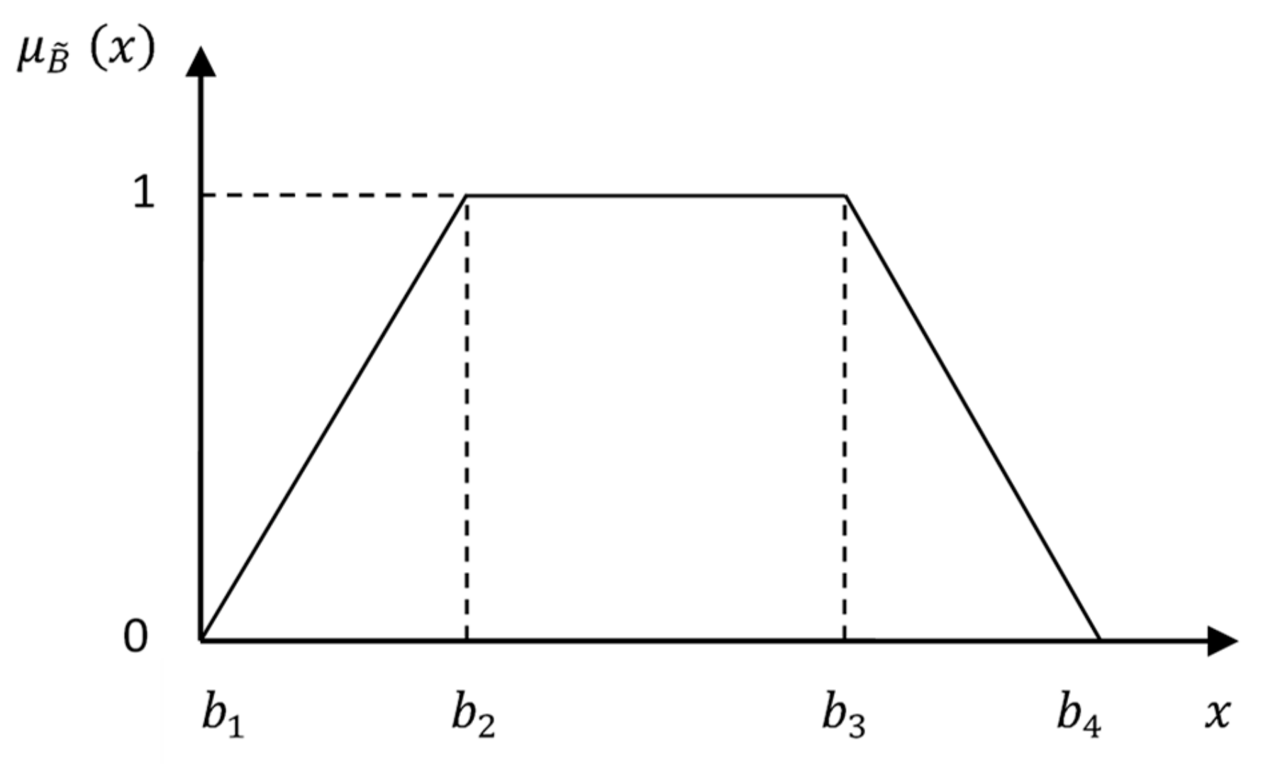
In regular figures, the area formed by the values of the fuzzy sets of the output variable was decomposed. To achieve this, the relationship between the membership grade of two adjacent fuzzy sets was analyzed, thereby defining two cases: The first case implied that the membership grade of the first fuzzy set was less than or equal to the value of belonging to the second set. For the second case, the membership grade of the first fuzzy set was greater than the membership grade of the second set. Four regular figures regarding the relationship between two adjacent fuzzy sets were formed.

2)

The surface of each figure obtained in step 1 was calculated.

3)

The centroid of each figure obtained in step 1 was determined.

4)

The total centroid was calculated, with the result being the value of the defuzzification of the response variable (fuzzy coefficient, ${\tilde{d}}_{i,j}$).

2.2.2. Computing the Optimal Route

The general distribution network is illustrated in Figure 7, including the source node (1), the sink node (n), the average time taken to travel from node i to node j ($c_{i,j}$), and the path from node i to node j ($X_{i,j}$).

To select the optimal route, we took into account travel time, travel time uncertainty, and type of street corner. We assumed that the arcs were a road set in the urban road network and the nodes were a set of street corners (Figure 7). Then, we considered the fuzzy coefficient, ${\tilde{d}}_{i,j}$, for each arc $\left(i,j\right)\in E$, $c_{i,j}$, the average time taken to travel from node i to node j, and $v_{i,j}$, the average time taken to cross street corners. Therefore, the fuzzy linear programming model was Equation (18).

$$\begin{array}{c}min Z={\displaystyle {\displaystyle \sum }_{i=1}^n}{\displaystyle {\displaystyle \sum }_{j\ne i}^n}{\widetilde{[d}}_{i,j}{c}_{i,j}+v_{i,j}]X_{i,j } \\ s. t. {\displaystyle {\displaystyle \sum }_{j\ne i}^n}{X}_{j,i} - {\displaystyle {\displaystyle \sum }_{j\ne i}^n}{X}_{i,j}=b_i, i=1,2,3,\dots , n\\ X_{i,j}\in \left\{0,1\right\} \forall i,j\end{array}$$

(18)

3. Results

3.1. Application to a Real Network

Figure 8 shows an application to a portion of the distribution area of a delivery company in the city of Tuxtla Gutierrez, Chiapas, Mexico. To demonstrate our approach, Figure 9 shows a portion of the distribution area with four blocks and nine street corners, where node 15 is the source, and node 43 is the sink.

Considering Chiapas’s traffic regulations, we used an average speed of 35 km/h for the avenues ($a{s}_1=9.72 m/s$), and an average speed of 20 km/h for the streets ($a{s}_2=5.55 m/s$). As shown in Figure 8, the distance of the arc was $a_{i,j}$ meters, therefore, the average travel time ($c_{i,j}$) in seconds was calculated using Equation (19).

$$c_{i,j}= \frac{a_{i,j}}{a{s}_k},$$

(19)

where k = 1 for the avenues, k = 2 for the streets, and $a_{i,j}$ represents the distance of the arc $\left(i,j\right)$.

The total time (in seconds) was calculated using Equation (20).

$$T{T}_{i,j}={\tilde{d}}_{i,j}{c}_{i,j}+v_{i,j}$$

(20)

Table 2. Time taken to cross street corners ($v_{i,j}$).

Type of Street Corner	Time in Seconds
Traffic light	50
Traffic light turn right	53
Traffic light turn left	57
No preference	8
Preference	3
Preference turn right	6
Preference turn left	7
One for one	4
One for one turn right	6
One for one turn left	6

illustrates the time in seconds used for each type of street corner. We sampled the distribution area to determine the average times for each type of street corner, as shown in Figure 8. For each intersection, we sampled 14 street corners at different times and noted 1519 observations. For the preferred street corner, we sampled four street corners at different times and noted 225 observations. For the non-preferred street corner, we sampled one street corner at different times and noted 50 observations. For traffic light intersections, we sampled four street corners at different times and noted 525 observations.

We analyzed the conditions of the fuzzy variables of the road and street corners of the real network by obtaining model parameters.

Table 3. Model parameters.

$\mathit{i}$	$\mathit{j}$	$\mathit{k}$	Time of Day	Traffic Density	${\mathit{a}}_{\mathit{i},\mathit{j}}$	${\mathit{c}}_{\mathit{i},\mathit{j}}$	${\tilde{\mathit{d}}}_{\mathit{i},\mathit{j}}$	${\tilde{\mathit{d}}}_{\mathit{i},\mathit{j}}{\mathit{c}}_{\mathit{i},\mathit{j}}$	${\mathit{v}}_{\mathit{i},\mathit{j}}$	$\mathit{T}\mathit{o}\mathit{t}\mathit{a}\mathit{l} \mathit{T}\mathit{i}\mathit{m}\mathit{e}$
15	16	2	13:36:57	2	80	14	3.21	44.94	4	48.94
15	28	2	13:36:57	1.1	98	18	2.06	37.08	6	43.08
16	17	2	13:36:57	1.1	83	15	2.06	30.90	4	34.90
17	30	2	13:36:57	2	94	17	3.21	54.57	6	60.57
28	29	1	13:36:57	2.1	83	9	4.21	37.89	50	87.89
28	41	2	13:36:57	2	102	18	3.21	57.78	53	110.78
29	16	2	13:36:57	2	99	18	3.21	57.78	53	110.78
29	28	1	13:36:57	2.1	83	9	4.21	37.89	50	87.89
29	30	1	13:36:57	2.1	79	8	4.21	33.68	50	83.68
30	29	1	13:36:57	2.1	79	8	4.21	33.68	50	83.68
30	43	2	13:36:57	2	100	18	3.21	57.78	53	110.78
41	42	2	13:36:57	1.1	81	15	2.06	30.90	4	34.90
42	29	2	13:36:57	2	101	18	3.21	57.78	6	63.78
42	43	2	13:36:57	1.8	81	15	3.05	45.75	4	49.75

shows the time of day and traffic density fuzzy variables and calculated the parameters $a_{i,j}$, $c_{i,j}$, ${\tilde{d}}_{i,j}$, ${\tilde{d}}_{i,j}{c}_{i,j}$, $v_{i,j}$, and total time ($T{T}_{i,j}$).

As shown in Table 3, node i was the initial node of arc $\left(i,j\right)$ and node j was the final node. For arc (15,16), node 15 was the initial node and node 16 was the final node. For arc (15,16), the type of road was a street, therefore k = 2 and $a{s}_2=5.55$ m/s. For arc (15,16), the street length was $a_{15,16}$ = 80 meters. Equation (19) was therefore used.

$$c_{15,16}= \frac{a_{15,16}}{a{s}_2}=\frac{80}{5.55}\approx 14 seconds$$

The time of day variable determined the scheduled goods delivery. In this study, the scheduled time of day was 13:36:57.

The traffic density variable was obtained via the following steps: Firstly, we considered the definition of the linguistic labels, as described in Section 2.1, to assign a real value ($1\le y\le 3$) to the $y$ fuzzy variable, i.e., traffic density, for each arc/street. Then, we designed a travel time study for each arc/street, with the purpose of adjusting the values. If necessary, we adjusted the value assigned to the fuzzy variable.

For arc (15,16), the roads next to the vehicular flow were located around shopping malls, therefore the fuzzy variable traffic density was 2. The fuzzy coefficient, (${\tilde{d}}_{i,j}$), was computed using the time of day and traffic density fuzzy variables, as described in Section 2.1, therefore ${\tilde{d}}_{15,16}=3.21$.

For arc (15,16), the type of street corner was one for one, therefore $v_{15,16}$ = 4 seconds. The total time was computed using Equation (20).

$$T{T}_{15,16}={\tilde{d}}_{15,16}{c}_{15,16}+v_{15,16}=44.94+4=48.94 seconds$$

The fuzzy linear programming problem for the application to the network was applied to Equations (6) and (18), therefore,

$$\begin{array}{c}\begin{array}{c}minZ= 48.94X_{15,16}+43.08X_{15,28}+34.90X_{16,17}+60.57X_{17,30}+87.89X_{28,29}+110.78X_{28,41}+110.78X_{29,16}\\ +87.89X_{29,28}+83.68X_{29,30}+83.68X_{30,29}+110.78X_{30,43}+34.90X_{41,42}+63.78X_{42,29}+49.75X_{42,43}\end{array}\\ \begin{array}{cc}s.t. -X_{15,16}- X_{15,28}& = -1\hfill \\ X_{15,16}-X_{16,17}+X_{29,16}& =0\hfill \\ X_{16,17}-X_{17,30}& =0\hfill \\ X_{15,28}-X_{28,29}-X_{28,41}+X_{29,28}& =0\hfill \\ X_{28,29}-X_{29,16}-X_{29,28}+X_{42,29}& =0\hfill \\ X_{17,30}+X_{29,30}-X_{30,29}-X_{30,43}& =0\hfill \\ X_{28,41}-X_{41,42}& =0\hfill \\ X_{41,42}-X_{42,29}-X_{42,43}& =0\hfill \\ X_{30,43}+X_{42,43}& =1\hfill \\ X_{i,j}\in \left\{0,1\right\} \forall i,j& \end{array}\end{array}$$

(21)

We calculated the optimal solution of the FLP problem using a version of the LP simplex method.

Table 4. Fuzzy optimal solution.

Variable	Value	Cost (Time)
$X_{15,16}$	0	48.94
$X_{15,28}$	1	43.08
$X_{16,17}$	0	34.90
$X_{17,30}$	0	60.57
$X_{28,29}$	0	87.89
$X_{28,41}$	1	110.78
$X_{29,16}$	0	110.78
$X_{29,28}$	0	87.89
$X_{29,30}$	0	83.68
$X_{30,29}$	0	83.68
$X_{30,43}$	0	110.78
$X_{41,42}$	1	34.90
$X_{42,29}$	0	63.78
$X_{42,43}$	1	49.75
$Z$	238.51

and Figure 10 show the optimal path {(15,28), (28,41), (41,42), (42,43)} and time in seconds. The computed optimal travel time was 00:03:58.51 (238.51 seconds).

We used Equation (21) to pose the fuzzy linear programming model for the network. Then, we calculated the optimal solution of the FLP problem. The computed optimal time of the FLP (00:03:58) was different to the time computed for the LP (00:02:13). Moreover, the time computed for the FLP was closer to the observed travel time (00:04:17).

3.2. Results Analysis

To analyze the reliability of the model, we designed a studio with 21 real network observations from a portion of a distribution area for a delivery company in the city of Tuxtla Gutierrez, Chiapas, Mexico, consisting of 68 blocks and 92 street corners (Figure 8). The source node was node 15 and the sink node was scheduled.

Table 5. Results obtained.

Route	Schedule	Real Travel Time	Calculated Time of the Classical Model (LP)	Absolute Percentage Error (LP) (%)	Calculated Time of the Fuzzy Model (FLP)	Absolute Percentage Error (FLP) (%)
15–13	6:22:17	0:05:29	0:03:37	34.04	0:03:53	29.18
15–13	14:28:37	0:07:35	0:03:37	52.31	0:06:37	12.75
15–13	19:03:55	0:02:51	0:03:37	26.90	0:03:11	11.70
15–40	10:15:26	0:04:17	0:03:47	11.67	0:04:34	6.61
15–40	13:49:21	0:07:35	0:03:47	50.11	0:07:05	6.59
15–40	21:47:33	0:02:50	0:03:47	33.53	0:02:34	9.41
15–50	7:15:30	0:04:25	0:03:42	16.23	0:04:41	6.04
15–50	11:45:17	0:04:11	0:03:42	11.55	0:04:41	11.95
15–50	23:08:05	0:02:35	0:03:42	43.23	0:02:46	7.10
15–59	7:26:02	0:05:37	0:04:03	27.89	0:05:56	5.64
15–59	17:25:32	0:04:34	0:04:03	11.31	0:04:21	4.74
15–59	20:21:59	0:03:19	0:04:03	22.11	0:03:03	8.04
15–64	8:01:19	0:06:32	0:04:23	32.91	0:06:02	7.65
15–64	13:54:58	0:08:58	0:04:23	51.12	0:08:39	3.53
15–64	20:31:44	0:02:58	0:04:23	47.75	0:03:15	9.55
15–82	10:06:48	0:04:44	0:03:15	31.34	0:04:22	7.75
15–82	14:03:51	0:07:02	0:03:15	53.79	0:06:34	6.64
15–82	22:47:33	0:01:58	0:03:15	65.25	0:02:31	27.97
15–88	5:32:28	0:06:38	0:04:27	32.91	0:06:51	3.27
15–88	13:36:57	0:10:49	0:04:27	58.86	0:10:15	5.24
15–88	18:04:30	0:05:53	0:04:27	24.36	0:05:17	10.20

shows the source node and the sink node in ascending order.

We computed the optimal solution with fuzzy linear programming for each day and executed the route following the optimal path found in the FLP. We also calculated the optimal solution using linear programming. The absolute percentage error (APE) was calculated using Equation (22).

$$APE=\frac{\left|RT-CT\right|}{RT}*100$$

(22)

where RT is the real time of travel, CT is the calculated time using the classical model or the calculated time using the fuzzy model.

Table 5 shows the route, the schedule, the real travel time, the calculated time of the classical model (LP), the absolute percentage error using LP, the calculated time of the fuzzy model (FLP), and the absolute percentage error using FLP.

We observed that the mean absolute percentage error of the classical model (LP) was 35.20%, while the mean absolute percentage error of the fuzzy model (FLP) was 9.60%. Moreover, the maximum absolute percentage error of the classical model was 65.25%, whereas the maximum absolute percentage error of the fuzzy model was 29.18%. Furthermore, the minimum absolute percentage error of the classical model was 11.31%; meanwhile, the minimum absolute percentage error of the fuzzy model was 3.27%. Finally, the variance of the absolute percentage error of the classical model was 264.14%, whilst the variance of the absolute percentage error of the fuzzy model was 46.57%.

We also attempted to determine whether the calculated time of the fuzzy model was adjusted for the real travel time. For the statistical analysis between the mean real travel time and the mean time calculated for FLP, we used paired t-tests, where α = 5%. We proposed a null hypothesis ($H_0$) and an alternative hypothesis ($H_1$).

$$\begin{array}{c}{H}_0: {\mu }_{RT}-{\mu }_{CT}=0\\ H_1: {\mu }_{RT}-{\mu }_{CT}\ne 0\end{array},$$

where ${\mu }_{RT}$ is the mean real travel time and ${\mu }_{CT}$ is the mean time calculated from the FLP.

Next, we evaluated the paired t-tests.

Table 6. Paired t-test for the mean real travel time vs. the calculated time from fuzzy linear programming (FLP).

	Real Travel Time	Calculated Time from FLP
Mean	5.277777777	5.101587301
Variance	5.247425925	4.260914021
Observations	21	21
Hypothesized Mean Difference	0
Df	20
t-stat	1.506943922
p-value	0.147458176
t-critical	2.085963447

shows the paired t-tests used to ascertain whether the null hypothesis (i.e., that the mean real travel time and mean time calculated from FLP were equal) was accepted or rejected. The p-value determined statistical significance.

Table 6 shows that the p-value (0.1475) was of a higher significance level (0.05) and that the t-stat (calculated statistic) was lower than the t-critical (t distribution table). Therefore, there was not sufficient statistical evidence to reject the null hypothesis. Hence, it was concluded that the mean real travel time was statistically equal to the mean calculated time in the proposed model. Therefore, the proposed model (FLP) adjusted to the travel time of the urban road network in this study.

Next, we aimed to determine whether the absolute percentage error of the classical model (LP) was higher than the absolute percentage error of the proposed model (FLP). For the statistical analysis, we used paired t-tests where α = 5%. We proposed a null hypothesis ($H_0$) and an alternative hypothesis ($H_1$).

$$\begin{array}{c}{H}_0: {\mu }_{LP}-{\mu }_{FLP}=0\\ H_1: {\mu }_{LP}-{\mu }_{FLP}>0\\ \end{array},$$

where ${\mu }_{LP}$ was the mean absolute percentage error of LP and ${\mu }_{FLP}$ was the mean absolute percentage error of FLP.

Table 7. Paired t-test for mean absolute percentage error of linear programming (LP) vs. the absolute percentage error from fuzzy linear programming.

	Absolute Percentage Error (LP)	Absolute Percentage Error (FLP)
Mean	35.199228509	9.597056757
Variance	264.135940142	46.574056590
Observations	21	21
Hypothesized Mean Difference	0
Df	20
t-stat	7.284123131
p-value	2.403528976 × 10−7
t-critical	1.724718243

shows the paired t-tests used to ascertain whether the null hypothesis (i.e., that the mean absolute percentage error of the classical model and mean absolute percentage error of fuzzy model were equal) was accepted or rejected.

Table 7 shows that the p-value (2.4035 × 10⁻⁷) was less than the significance level (0.05), and that the t-stat (calculated statistic) was higher than the t-critical (t distribution table), therefore the null hypothesis was rejected. Accordingly, it was concluded that the mean absolute percentage error of the LP was higher than the means absolute percentage error of the FLP, i.e., the proposed model. Therefore, the proposed model (FLP) predicted real travel times better than the classical model (LP) in this study, thereby providing more reliable travel times in the urban road network.

In this approach, we considered fuzzy variables that influence the travel times of routes within an urban area. These fuzzy variables were not considered in the classic models, thus, we obtained values closer to the real route times with this proposal.

4. Discussion

In this paper, the implementation of fuzzy logic allowed us to model the uncertainty of the route optimization problem that occurs when delivering products in an urban road network through two linguistic variables, namely, time of day and traffic density. By adjusting the travel times and applying fuzzy linear programming, we computed the shortest path, thereby providing a more reliable result than the results of the classical model (Table 5), with a mean absolute percentage error (MAPE) of 9.60% in this study. However, if conditions change due to the fuzzy variables, it is possible that the optimal route will change.

This approach provides a good tool for route selection when delivering products in urban road networks, increasing the reliability of the transportation system through route optimization. In this study, the maximum absolute percentage error of the classical model (LP) was reduced by 36.07%. By applying the proposed method to a larger proportion of the distribution area of a delivery company, we expect even better results.

5. Conclusions

The shortest path problem is important for practical applications, e.g., in route optimization for a delivery company. The use of fuzzy logic to consider arc weights as a non-deterministic value further improves the obtained results.

With the classic models, the optimal route of product delivery is determined. However, this optimal route is unable to change during the analysis period, regardless of whether the delivery conditions are changing. On the other hand, with the approach raised in this investigation, the determined optimal route of goods delivery is able to adjust to different conditions, i.e., the time of day and traffic density fuzzy variables. With this approach, we were able to calculate travel times that were closer to the real travel times of the routes.

In this study, we observed that the optimal route sometimes changed according to the changing fuzzy variables. Therefore, with this approach, we determined the optimal route of goods delivery for the different fuzzy variable conditions, which guaranteed the shortest travel time for each delivery. Minimizing delivery route travel times is expected to reduce pollution and the level of noise generated by delivery units and increase the transfer capacity, thereby contributing to sustainable transport.

Furthermore, it is worth bearing in mind that when the conditions of the urban road network change, it is necessary to adapt the membership function’s fuzzy variable parameters to the new conditions.

This paper puts forward elements to help consider a larger number of fuzzy variables in future projects. Different uncertain elements, such as rain and the condition of the streets, among others, could be analyzed. We suggest amplifying the street corner crossing time used in this study in order to consider the uncertain factors that affect street corner crossing time.

This study empowers workers to make better decisions in the area of distribution regarding their travel routes.

References

1. Bellman, E. On a routing problem. Q. Appl. Math. 1958, 16, 87–90. [Google Scholar] [CrossRef]
2. Dijkstra, E.W. A note on two problems in connection with graphs. Numer. Math. 1959, 1, 269–271. [Google Scholar] [CrossRef]
3. Dantzig, G.B. On the shortest route through a network. Manag. Sci. 1960, 6, 187–190. [Google Scholar] [CrossRef]
4. Floyd, R.W. Algorithm 97: Shortest path. Commun. ACM 1962, 5, 345. [Google Scholar] [CrossRef]
5. Butas, L.F. A directionally oriented shortest path algorithm. Transp. Res. 1968, 2, 253–268. [Google Scholar] [CrossRef]
6. Johnson, D.B. Efficient algorithms for shortest paths in sparse networks. J. Assoc. Comput. Mach. 1977, 24, 1–13. [Google Scholar] [CrossRef]
7. Zhan, F.B.; Noon, C.E. Shortest path algorithms: An evaluation using real road networks. Transp. Sci. 1998, 32, 65–73. [Google Scholar] [CrossRef]
8. Zamirian, M.; Farahi, M.; Nazemi, H.A.R. An applicable method for solving the shortest path problems. Appl. Math. Comput. 2007, 190, 1479–1486. [Google Scholar] [CrossRef]
9. An, P.T.; Hai, N.N.; Hoai, T.V. Direct multiple shooting method for solving approximate shortest path problems. J. Comput. Appl. Math. 2013, 244, 67–76. [Google Scholar] [CrossRef]
10. Bode, C.; Irnich, S. The shortest-path problem with resource constraints with (k,2)-loop elimination and its application to the capacitated arc-routing problem. Eur. J. Oper. Res. 2014, 238, 415–426. [Google Scholar] [CrossRef]
11. Duque, D.; Lozano, L.; Medaglia, A.L. An exact method for the biobjective shortest path problem for large-scale road networks. Eur. J. Oper. Res. 2015, 242, 788–797. [Google Scholar] [CrossRef]
12. Marinakis, Y.; Migdalas, A.; Sifaleras, A. A hybrid particle swarm optimization-variable neighborhood search algorithm for constrained shortest path problems. Eur. J. Oper. Res. 2017, 261, 819–834. [Google Scholar] [CrossRef]
13. Rostami, B.; Chassein, A.; Hopf, M.; Frey, D.; Buchheim, C.; Malucelli, F.; Goerigk, M. The quadratic shortest path problem: Complexity, approximability, and solutions methods. Eur. J. Oper. Res. 2018, 268, 473–485. [Google Scholar] [CrossRef]
14. Arun Prakash, A. Pruning algorithm for the least expected travel time path on stochastic and time-dependent networks. Transp. Res. Part B 2018, 108, 127–147. [Google Scholar] [CrossRef]
15. Chen, B.Y.; Li, Q.; Lam, W.H.K. Finding the k reliable shortest paths under travel time uncertainty. Transp. Res. Part B 2016, 94, 111–135. [Google Scholar] [CrossRef]
16. Strehler, M.; Merting, S.; Schwan, C. Energy-efficient shortest routes for electric and hybrid vehicles. Transp. Res. Part B 2017, 103, 189–203. [Google Scholar] [CrossRef]
17. Shi, N.; Zhou, S.; Wang, F.; Tao, Y.; Liu, L. The multi-criteria constrained shortest path problem. Transp. Res. Part E 2017, 101, 13–29. [Google Scholar] [CrossRef]
18. Zhang, Y.; Shen, Z.M.; Song, S. Lagrangian relaxation for the reliable shortest path problem with correlated link travel times. Transp. Res. Part B 2017, 104, 501–521. [Google Scholar] [CrossRef]
19. Cooke, K.L.; Halsey, E. The Shortest Route Through a Network with Time-Dependent Internodal Transit Times. J. Math. Anal. Appl. 1966, 14, 493–498. [Google Scholar] [CrossRef]
20. Hernandes, F.; Lamata, M.T.; Verdegay, J.L.; Yamakami, A. The shortest path problem on networks with fuzzy parameters. Fuzzy Sets Syst. 2007, 158, 1561–1570. [Google Scholar] [CrossRef]
21. Deng, Y.; Chen, Y.; Zhang, Y.; Mahadevan, S. Fuzzy Dijkstra algorithm for shortest path problem under uncertain environment. Appl. Soft Comput. 2012, 12, 1231–1237. [Google Scholar] [CrossRef]
22. Dou, Y.; Zhu, L.; Wang, H.S. Solving the fuzzy shortest path problem using multi-criteria decision method based on vague similarity measure. Appl. Soft Comput. 2012, 12, 1621–1631. [Google Scholar] [CrossRef]
23. Kok, A.L.; Hans, E.W.; Schutten, J.M.J. Vehicle routing under time-dependent travel times: The impact of congestion avoidance. Comput. Oper. Res. 2012, 39, 910–918. [Google Scholar] [CrossRef]
24. Farhanchi, M.; Hassanzadeh, R.; Mahdavi, I.; Mahdavi-Amiri, N. A modified ant colony system for finding the expected shortest path in networks with variable arc lengths and probabilistic nodes. Appl. Soft Comput. 2014, 21, 491–500. [Google Scholar] [CrossRef]
25. Lakouari, N.; Ez-Zahraouy, H.; Benyoussef, A. Traffic flow behavior at a single lane roundabout as compared to traffic circle. Phys. Lett. A 2014, 378, 3169–3176. [Google Scholar] [CrossRef]
26. Frank, H. Shortest paths in probabilistic graphs. Oper. Res. 1969, 17, 583–599. [Google Scholar] [CrossRef]
27. Mirchandani, P.B. Shortest distance and reliability of probabilistic networks. Comput. Oper. Res. 1976, 3, 347–355. [Google Scholar] [CrossRef]
28. Sigal, C.E.; Pritsker, A.A.B.; Solberg, J.J. The stochastic shortest route problem. Oper. Res. 1980, 28, 1122–1129. [Google Scholar] [CrossRef]
29. Noorizadegan, M.; Chen, B. Vehicle routing with probabilistic capacity constraints. Eur. J. Oper. Res. 2018, 270, 544–555. [Google Scholar] [CrossRef]
30. Dubois, D.; Prade, H. Algorithmes de plus courts chemins pour traiter des donnees floues. RAIRO Oper. Res. 1978, 12, 213–227. [Google Scholar] [CrossRef]
31. Chanas, S.; Kamburowski, J. The fuzzy shortest route problem. In Interval and Fuzzy Mathematics; Albrycht, J., Wisniewski, H., Eds.; Technology University of Poznan: Poznan, Poland, 1983; pp. 35–41. [Google Scholar]
32. Chanas, S.; Delgado, M.; Verdegay, J.L.; Vila, M.A. Fuzzy optimal flow on imprecise structures. Eur. J. Oper. Res. 1995, 83, 568–580. [Google Scholar] [CrossRef]
33. Klein, C.M. Fuzzy shortest paths. Fuzzy Sets Syst. 1991, 39, 27–41. [Google Scholar] [CrossRef]
34. Dey, A.; Pal, A.; Pal, T. Interval type 2 Fuzzy Set in Fuzzy Shortest Path Problem. Mathematics 2016, 4, 62. [Google Scholar] [CrossRef] [Green Version]
35. Tajdin, A.; Mahdavi, I.; Amiri, N.M.; Sadeghpour-Gildeh, B. Computing a fuzzy shortest path in a network with mixed fuzzy arc lengths using α-cuts. Comput. Math. Appl. 2010, 60, 989–1002. [Google Scholar] [CrossRef] [Green Version]
36. Ramazani, H.; Shafahi, Y.; Seyedabrishami, S.E. A Shortest Path Problem in an Urban Transportation Network Based on Driver Perceived Travel Time. Trans. A Civ. Eng. 2010, 17, 285–296. [Google Scholar]
37. Dai, L.; Fan, L.; Sun, L. Aggregate production planning utilizing a fuzzy linear programming. J. Integr. Des. Process Sci. 2003, 7, 81–95. [Google Scholar]
38. Fung, R.; Tang, J.; Wang, D. Multiproduct Aggregate Production Planning with Fuzzy Demands and Fuzzy Capacities. IEEE Trans. Syst. Man Cybern. Part A 2003, 33, 302–313. [Google Scholar] [CrossRef]
39. Sheng-Tun, L.; Yi-Chung, C. Deterministic Fuzzy Time Series Model for Forecasting Enrollments. Comput. Math. Appl. 2007, 53, 1904–1920. [Google Scholar]
40. Castillo, O.; Melin, P. Automated mathematical modelling for financial time series prediction combining fuzzy logic and fractal theory. In Soft Computing for Financial Engineering; Kacprzyk, J., Ed.; Springer: Berlin/Heidelberg, Germany, 1999; pp. 93–106. [Google Scholar]
41. Escobar-Gómez, E.N.; Díaz-Núñez, J.J.; Taracena-Sanz, F.L. Model for Adjustment of Aggregate Forecasts using Fuzzy Logic. Ingeniería Investigación y Tecnología. 2010, 11, 289–302. [Google Scholar] [CrossRef] [Green Version]
42. Hosseini, R.; Dehmeshki, J.; Barman, S.; Mazinani, M.; Qanadi, S. A genetic type-2 fuzzy logic system for pattern recognition in computer aided detection system. In Proceedings of the 2010 IEEE World Congress on Computational Intelligence, Barcelona, Spain, 18–23 July 2010. [Google Scholar]
43. Deng, Y.; Shi, W.K.; Du, F.; Liu, Q. A new similarity measure of generalized fuzzy numbers and its application to pattern recognition. Pattern Recognit. Lett. 2004, 25, 875–883. [Google Scholar]
44. Bellman, R.E.; Kalaba, R.E.; Zadeh, L.A. Abstraction and pattern classification. J. Math. Anal. Appl. 1966, 13, 1–7. [Google Scholar] [CrossRef]
45. Mitra, S.; Pal, S.K. Fuzzy sets in pattern recognition and machine intelligence. Fuzzy Sets Syst. 2005, 156, 381–386. [Google Scholar] [CrossRef] [Green Version]
46. Pedrycz, W. Fuzzy sets in pattern recognition: Accomplishments and challenges. Fuzzy Sets Syst. 1997, 90, 171–176. [Google Scholar] [CrossRef]
47. Mitchell, H.B. Pattern recognition using type-II fuzzy sets. Inf. Sci. 2005, 170, 409–418. [Google Scholar] [CrossRef]
48. Tizhoosh, H.R. Image thresholding using type II fuzzy sets. Pattern Recognit. 2005, 38, 2363–2372. [Google Scholar] [CrossRef]
49. Das, S. Pattern Recognition using the Fuzzy c-means Technique. Int. J. Energy Inf. Commun. 2013, 4, 1–14. [Google Scholar]
50. Zadeh, L.A. Outline of a New Approach to the Analysis of Complex Systems and Decision Processes. IEEE Trans. Syst. Man Cybern. 1973, 3, 28–44. [Google Scholar] [CrossRef]
51. Bellman, R.E.; Zadeh, L.A. Decision-making in a fuzzy environment. Manag. Sci. 1970, 17, 141–164. [Google Scholar] [CrossRef]
52. Mardani, A.; Jusoh, A.; Zavadskas, E.K. Fuzzy multiple criteria decision-making techniques and applications-two decades review from 1994 to 2014. Expert Syst. Appl. 2015, 42, 4126–4148. [Google Scholar] [CrossRef]
53. Boulmakoul, A. Generalized path-finding algorithms on semirings and the fuzzy shortest path problem. J. Comput. Appl. Math. 2004, 162, 263–272. [Google Scholar] [CrossRef] [Green Version]
54. Mahdavi, I.; Nourifar, R.; Heidarzade, A.; Amiri, N.M. A dynamic programming approach for finding shortest chains in a fuzzy network. Appl. Soft Comput. 2009, 9, 503–511. [Google Scholar] [CrossRef]
55. Ghatee, M.; Hashemi, S.M.; Zarepisheh, M.; Khorram, E. Preemptive priority based algorithms for fuzzy minimal cost flow problem: An application in hazardous materials transportation. Comput. Ind. Eng. 2009, 57, 341–354. [Google Scholar] [CrossRef]
56. Ghatee, M.; Hashemi, S.M. Application of fuzzy minimum cost flow problems to network design under uncertainty. Fuzzy Sets Syst. 2009, 160, 3263–3289. [Google Scholar] [CrossRef]
57. Keshavarz, E.; Khorram, E. A fuzzy shortest path with the highest reliability. J. Comput. Appl. Math. 2009, 230, 204–212. [Google Scholar] [CrossRef] [Green Version]
58. Marien, E.J. The application of linear programming to a distribution system orientated toward service. Int. J. Phys. Distrib. 1972, 3, 191–204. [Google Scholar] [CrossRef]
59. Ali, M.A.M.; Sik, Y.H. Transportation problem: A special case for linear programming problems in mining engineering. Int. J. Min. Sci. Technol. 2012, 22, 371–377. [Google Scholar] [CrossRef]
60. García, J.; Florez, J.E.; Torralba, A.; Borrajo, D.; López, C.L.; García-Olaya, A.; Sáenz, J. Combining linear programming and automated planning to solve intermodal transportation problems. Eur. J. Oper. Res. 2013, 227, 216–226. [Google Scholar] [CrossRef]
61. Luathep, P.; Sumalee, A.; Lam, W.H.K.; Li, Z.; Lo, H.K. Global optimization method for mixed transportation network design problem: A mixed-integer linear programming approach. Transp. Rese. Part B Methodol. 2011, 45, 808–827. [Google Scholar] [CrossRef]
62. Faddel, S.; Aldeek, A.; Al-Awami, A.T.; Sortomme, E. ZAl-Hamouz, Ancillary Services Bidding for Uncertain Bidirectional V2G Using Fuzzy Linear Programming. Energy 2018, 160, 986–995. [Google Scholar] [CrossRef]
63. Zimmermann, H.J. Fuzzy programming and linear programming with several objective functions. Fuzzy Sets Syst. 1978, 1, 45–56. [Google Scholar] [CrossRef]
64. Okada, S.; Soper, T. A shortest path problem on a network with fuzzy arc length. Fuzzy Sets Syst. 2000, 109, 129–140. [Google Scholar] [CrossRef]
65. Buckley, J.J. Possibilistic linear programming with triangular fuzzy numbers. Fuzzy Sets Syst. 1988, 26, 135–138. [Google Scholar] [CrossRef]
66. Foulds, L.R.; Nascimento, H.A.D.D.; Calixto, I.C.A.C.; Hall, B.R.; Longo, H. A fuzzy set-based approach to origin–destination matrix estimation in urban traffic networks with imprecise data. Eur. J. Oper. Res. 2013, 231, 190–201. [Google Scholar] [CrossRef]
67. Ebrahimnejad, A.; Tavana, M. A novel method for solving linear programming problems with symmetric trapezoidal fuzzy numbers. Appl. Math. Model. 2014, 38, 4388–4395. [Google Scholar] [CrossRef]
68. Zhu, G.; Song, K.; Zhang, P.; Wang, L. A traffic flow state transition model for urban road network based on Hidden Markov Model. Neurocomputing 2016, 214, 567–574. [Google Scholar] [CrossRef] [Green Version]
69. Tian, Z.; Jia, L.; Dong, H.; Su, F.; Zhang, Z. Analysis of Urban Road Traffic Network Based on Complex Network. Procedia Eng. 2016, 137, 537–546. [Google Scholar] [CrossRef] [Green Version]
Figure 1. Triangular fuzzy number.
Sustainability 11 06665 g001
Figure 2. Trapezoidal fuzzy number.
Sustainability 11 06665 g002
Figure 3. General network.
Sustainability 11 06665 g003
Figure 4. Time of day fuzzy variable.
Sustainability 11 06665 g004
Figure 5. Traffic density fuzzy variable.
Sustainability 11 06665 g005
Figure 6. Adjusted time output fuzzy variable.
Sustainability 11 06665 g006
Figure 7. Diagram of the distribution network.
Sustainability 11 06665 g007
Figure 8. Diagram of the application zone.
Sustainability 11 06665 g008
Figure 9. Diagram of a portion of the distribution area.
Sustainability 11 06665 g009
Figure 10. Diagram of the optimal solution.
Sustainability 11 06665 g010