What Drives Green Fodder Supply in China?—A Nerlovian Analysis with LASSO Variable Selection

Abstract

To understand key factors that drive China’s green fodder supply, this study estimates a Nerlovian partial-adjustment model, using provincial-level panel data spanning two decades (1997–2016). Based on a set of explanatory variables selected by the LASSO (Least Absolute Shrinkage and Selection Operator) method, estimation of the Nerlovian model by the system-GMM (Generalized Method of Moments) method yields three key findings. First, while farmers’ previous cultivation decisions on green fodder supply strongly predict their current decisions, without the influence of other drivers, China’s green fodder supply tends to decline over time. Second, among the identified drivers, government policy plays the most significant role—the availability of subsidies for cultivation of green fodder crops raises the sown area of green fodder crops by more than 30 percent. In contrast, farmer’s sown-area decision is only modestly responsive to price incentives. Finally, while the stock of fixed capital inputs (e.g., number of combine harvesters) and natural disasters (e.g., floods) both affect green fodder supply, their impacts are small.

1. Introduction

Dramatic increases in wealth and food availability in China, owing to its economic reforms and the resulting rapid economic growth, have greatly transformed Chinese consumers’ food consumption patterns. Official statistics indicate that per capita consumption of animal products (including meat, eggs, milk, and aquatic products) among urban households rose from 44.4 to 81.1 kilograms during the period of 1997–2017, with a growth rate of 82.7% [1]. Meanwhile, the focus of food demand has shifted from quantity targets, e.g., to ensure food security, to quality aspects, such as food variety, nutritional content, and food safety [2,3]. In particular, shocked by a series food-safety scandals, including the notorious incident of melamine-contaminated infant formulas in 2008, Chinese consumers have started to pay considerable attention to information on the manufacturer, nutrition content, and production process of animal products [4]. All these call for a healthy and sustainable development of China’s livestock sector.

Adequate supply of high-quality green fodder crops—i.e., fresh crops that are rich in water and nutrients [5], including natural grass or artificial herbage (e.g., ryegrass, alfalfa and silage corn), leafy fodder (e.g., sweet potato vines), aquatic feed (e.g., water hyacinth), wild weeds, and wild vines [6])—plays a key role in the sustainable development of a country’s livestock sector [7,8,9]. However, the sown area of green fodder crops accounted for less than 2% of the total area of farm crops in China in the past two decades, and this percentage has declined to below 1% since 2012 [1]. Largely due to the rapidly growing demand for livestock products in the recent decade [10,11], China’s green fodder demand has outgrown its domestic supply. The resulting shortage in green fodder supply has led China’s livestock husbandry to rely heavily on feed grain, straw, and other feedstuffs as substitutes for green fodder, which, in turn, created a number of problems in China’s agri-food system. Firstly, the inferior quality of these substitute feedstuffs (relative to that of green fodder) substantially lowers the production efficiency of China’s livestock sector. In particular, due to insufficient green fodder content in dairy cow rations, the average lactation yield of Chinese dairy cows (5 tons) is about 45% lower than that of their American counterparts (9 tons) [9]. The low quality of livestock products also creates room for illegal practice among irresponsible food providers, who often use illegal additives and preservatives to increase sales, whereby imposing a serious burden of health risks on Chinese consumers [2,3,4]. Secondly, the ever-heavier reliance of China’s livestock sector on feed grains has deteriorated the pressing problem of “competition for grain between humans and animals” in China [12]. As indicated by official estimates, the amount of feed grains consumed in China accounted for more than 40% of the total national grain consumption in the past decade [13]. Finally, facing insufficient domestic green fodder supply, China has turned to the international market to meet its domestic demand, importing 1.72 million tons of green fodder from overseas in 2016 alone [14]. The heavy dependence on international supply introduces substantial risks to China’s livestock production system. For instance, the unexpected increase in tariff and global supply shortage in 2018 caused forage costs in China to jump up by 6% [15].

In response to these problems, the Chinese government has set up an agenda for developing a sustainable, herbivorous and grain-saving stockbreeding system [16]. Subsidies for planting green fodder crops, as part of the Returning Farmland to Forests and Grassland (RFFG) initiative, were also provided to farmers to help achieve this goal [17]. Yet before specific action plans can be designed and carried out to achieve this goal, two fundamental questions need to be answered: what are the fundamental drivers of green fodder supply in China? And, among these drivers, which are the most relevant ones: price factors (e.g., factor prices and output prices of green fodder and its competitor crops) or non-price factors, such as technology (e.g., availability of high-yield varieties), natural conditions (e.g., flood and drought occurrences), or government policies (e.g., green fodder planting subsidies)? Unfortunately, the existing literature on green fodder supply has largely failed to provide conclusive answers to these questions. For instance, previously estimated impacts of output price, the most important building block of any crop supply models, vary from being significantly positive [18] to being irrelevant [19]. The role of governmental policies is also unclear, varying from being “strong” [20] to being “negligible” [21]. These discrepancies in findings are presumably due to the fact that previous studies were focused on different (and relatively small) regions in China with vastly different local conditions, which seriously limits the external validity of their findings. The conditioning on different explanatory variables also greatly reduces the comparability across different studies. In fact, this problem (of including different explanatory variables in the empirical model) also plagues the studies of agricultural supply responses in other contexts. For example, in a series of studies that estimated the acreage (supply) response of wheat in the United States [21,22,23,24], the role of governmental intervention programs vary greatly from being significantly negative [21,22,23] to being positive [24]. The specific drivers of wheat supply examined in these studies were also quite different. For example, Lidman and Bawden [21] considered the national wheat allotment and the announced loan rate to be key drivers of wheat supply in the U.S. Garst and Miller [22] considered diversion for payment and the market price of wheat in the preceding season as additional driving factors, while Morzuch et al. [23] and Krause et al. [24] further included prices of other crops and price risk in their respective models. Keeping in mind the problems existing in the international literature, and in the literature specifically on China, to depict a more comprehensive picture of the key drivers underlying China’s green-fodder supply, more-systematic analyses that (1) use data with a greater geographical coverage, (2) cover a longer time span, and (3) consider a larger set of potential factors, are clearly needed.

The present paper aims to fill this demand by estimating an expanded Nerlovian partial-adjustment model [25,26,27] of green fodder supply in China, based on provincial-level panel data spanning two decades (1997–2016); to reflect suppliers’ planting decisions more directly, our analysis focuses on the sown-area of green fodder (rather than the output of it). Special attention is paid to variable selection in the analysis. Note that, except for the basic variables specified in the original Nerlovian model [27,28,29], such as lagged output prices and lagged sown areas, theory is silent on what other factors should be included in the empirical model. Meanwhile, many previous researchers have considered other factors in their empirical models. For instance, Konyar and Knapp [30] examined the impacts of cost of production, availability of crop rotation technology, and prices of competing crops on the supply of alfalfa—a major green-fodder crop—in California, United States. Wang et al., [19] examined the impacts of prices of different competitor crops of alfalfa (i.e., maize, wheat and cotton) on alfalfa supply in China. Wang and Qian [18] estimated the impact of the price of maize, a substitute crop of alfalfa, on the sown area of alfalfa, and the impact of fertilizer use on alfalfa yield in China. Since the major categories of factors that may potentially affect green-fodder supply (e.g., input prices, prices of competitor crops, and areas affected by natural disasters) examined in previous studies involve more than 70 specific variables [29], we resort to the LASSO (Least Absolute Shrinkage and Selection Operator) method, a machine-learning algorithm developed by Tibshirani [31], to select the most relevant driving factors of China’s green fodder supply. In estimating the Nerlovian green fodder supply model, LASSO finds the coefficients of the explanatory variables that minimize the sum of squared residuals, plus a “penalty” function that penalizes the size of the model (defined over the sum of absolute values of the estimated coefficients), by setting the coefficients of some explanatory variables (which are part of the penalty function) to zero, leaving only the most relevant variables in the estimated model. Our LASSO procedure selects 21 variables out of the full set of 76 variables available in the data. Not only does the set of LASSO-selected variables cover most of the relevant categories of factors found in previous studies [18,19,30,32], such as sown areas of competitor crops, fixed (capital) inputs, and the availability of production services (proxied by the stock of agricultural machinery), it also includes a number of factors that have been neglected in most of the previous studies, such as natural disasters and subsidy policy.

Based on the LASSO-chosen variables, estimation of the Nerlovian model using the two-step system GMM (Generalized Method of Moments) method [33,34] reveals that, while both price and non-price factors matter for the sown area of green fodder crops in China, non-price factors play a more important role. First, while suppliers’ sown-area decision made in the previous year strongly predicts their decision in the current year, the estimated elasticity is slightly less than unity, suggesting that, without the influence of other drivers, green fodder supply in China tends to decline over time. Second, among the significant drivers we found, government policy, the availability of subsidies matters the most. It boosts the sown area of green fodder crops up by more than 30%. Suppliers’ sown-area decision is also responsive to price incentives, but not dramatically so—the estimated own-price elasticity is only about 0.21. Finally, while the stock of fixed capital inputs (e.g., the number of combine harvesters) and natural disasters (e.g., floods) both affect green folder supply in a statistically significant manner, their impacts are quite small in magnitude.

The remainder of this paper is organized as follows. The next section describes the data and develops an empirical framework for estimating drivers of green fodder supply in China. Section 3 reports computational and estimation results. Section 4 discusses the findings of the paper. The final section draws conclusions and points out several directions for future research.

2. Materials and Methods

2.1. Data Compilation

The dataset analyzed in this paper is a provincial-level panel dataset covering 27 provincial-level administration units (22 provinces and five autonomous regions) in mainland China for the period of 1997–2016, compiled from Provincial Statistical Yearbooks published in relevant years [1]. Four municipalities (namely, Beijing, Shanghai, Tianjin and Chongqing, which are also provincial-level administration units) are not included in the dataset, due to serious data-missing problems and their very limited sown areas of green fodder crops.

The variables used in the analysis can be subdivided into five categories (

Table 1. Potential driving factors of green fodder supply in China.

	All Originally Available Variables
Variable Category	(1) Variables not Selected by LASSO	(2) LASSO-selected Variables
(1) Lagged sown area (1000 hectares) [43 variables]	Total sown areas of: farm crops, grain crops, grain crops harvested in summer, grain crops harvested in autumn, cereal, rice, early rice, middle-season rice and single-cropping late rice, double-cropping late rice, wheat, winter wheat, spring wheat, corn, millet, jowar, other cereal, barley, beans, soja, mung, red bean, tubers, potato, oil-bearing crops, peanuts, rapeseeds, sesame, helianthus, benne, cotton, fiber crops, jute and ambary hemp, flax, hemp, ramee, sugar crops, sugarcane, beetroots, tobacco, flue-cured tobacco, vegetables, medicinal materials, other farm crops	Lagged sown area of: fiber crops (100), other cereal (100), other farm crops (100), jute and ambary hemp (95), mung (93), spring wheat (84), helianthus (69), winter wheat (69), hemp (49), peanuts (35), oil-bearing crops (11), rapeseeds (11)
(2) Price indices for agricultural production inputs (2007 price = 100) [14 variables]	Price indices for: farm hand tools, forage, commodity animals, semi-mechanized farm tools, mechanized farm machinery, mechanized farm machinery, chemical fertilizer, pesticide and its appliances, chemical pesticide, pesticide appliances, oil for farm machinery, other agricultural production inputs, agricultural seed, other agricultural production inputs (other than seed), price indices of agricultural production service	Price indices for: other means of agricultural production (other than seed) (96), service of agricultural production (96), semi-mechanized farm tools (49)
(3) Encouragement (subsidy) policy [1 variable]	Subsidy of green fodder cultivation (“Returning Farmland to Forests and Grass” (1999–2003))	Subsidy for green fodder cultivation (100)
(4) Areas affected by natural disasters area (1000 hectares) [10 variables]	Areas potentially covered by natural disasters, flood, drought, windstorm and hail, freeze injury; Areas seriously affected by natural disasters, flood, drought, windstorm and hail, freeze injury	Areas seriously affected by freeze injury (58), areas potentially covered by floods (58), areas seriously affected by floods (23)
(5) Agricultural machinery (year-end) [8 variables]	Number of: large and medium-sized agricultural tractors, small tractors, towing farm machinery of large and medium-sized agricultural tractors, towing farm machinery of small tractors, agricultural electronic engines, agricultural diesel engines, combine harvesters, motorized threshing machines	Number of: motorized threshing machines (49), combine harvesters (11)

Notes: Numbers in parentheses in the last column indicate the number of times these variables are selected out of the 100 LASSO simulations.

): (1) (lagged) sown areas of major crops that are potentially competitor crops or rotation crops of green fodder crops; (2) price indices for agricultural inputs; (3) policies such as subsidies for the cultivation of green fodder crops [12] and related directives stipulated in official documents and reports (especially, the No.1 Documents of the Central Government that focus on agricultural development) issued in relevant years; (4) areas affected by various natural disasters; (5) year-end numbers of major agricultural machines (as proxies for fixed inputs or capital stock in agricultural production).

A series of data manipulations were performed in preparing the dataset for estimation. First, all prices were deflated using production price indices, with the 2007 price being set as 100—the year of 2007 was chosen because it is the year with the fewest missing values. Second, all continuous variables were transformed into their logarithms to reduce to the problem of outliers and to obtain elasticity measures for ease of interpretation and comparison—a small constant, one, is added to the variables to avoid taking log of zeros. Third, since the variable selection method adopted in this paper (i.e., the LASSO method, discussed in more detail in the next section) does not support analytical samples with missing values, we imputed all missing values in our dataset using the “MICE (multivariate imputation by chained equations)” procedure developed by Buuren [35] and Buuren and Groothuis–Oudshoorn [36]. In the MICE procedure, each variable with missing values was modeled on the basis of other observed variables in the dataset, based on a series of linear regression models that were run to impute those missing values [37,38].

2.2. Analytical Framework

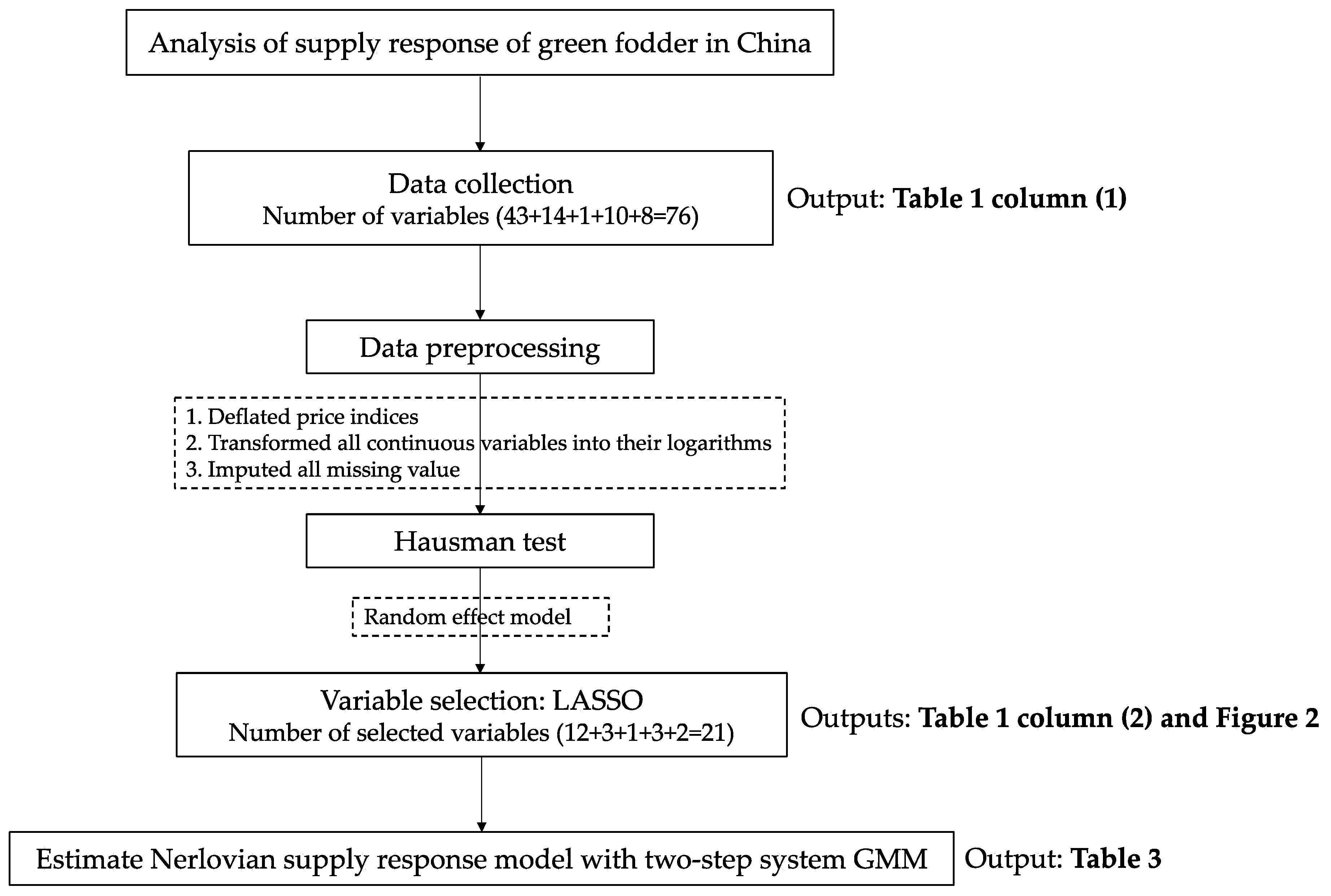
Figure 1 illustrates conceptually the procedure we undertook to analyze green fodder supply in China. Detailed descriptions of all analytical tools adopted in the analysis are provided in the following subsections. All results discussed in this paper are obtained using the Statistical Analysis software R 3.4.3.

2.2.1. The Nerlovian Supply-Response Model

Agricultural supply is usually modelled as the response of crop sown area (or output) to variations in price and other factors [27]. In order to study agricultural supply response, it is vital to properly define and measure farmers’ price expectations. Three price-expectation models have been devised and commonly adopted in the existing literature of supply response: the naïve price-expectation model, the adaptive price-expectation model, and the rational price-expectation model, which differ mainly in their assumptions on how farmers form their price expectations [39]. More specifically, the naïve price expectation model assumes that farmers do not have a learning process in forming their price expectation; rather, they make their crop planting decisions solely based on the market price realized in the previous time period [40]. The obvious limitation of this model is its ignorance of farmers’ price expectation. The adaptive price-expectation model relaxes the assumptions of the naïve price-expectation model, by allowing farmers’ crop planting decisions to be responsive to the expected price, rather than the realized one, and allowing the expected price to depend not only on the price realized in the last period but also on the prices realized in all past periods [25]; these relaxations certainly render the adaptive price-expectation model much more realistic (compared to the naïve price-expectation model). The rational price-expectation model further refines the adaptive price-expectation model by assuming that farmers adjust their price expectation based on all available information in the market, including information on the structure of the system that generates the data [29,41]. While theoretically compelling, the notion of rational price-expectation may not be easy to characterize and measure empirically, as it is determined by both supply and demand in the equilibrium, which imposes a heavy burden on data collection [29]. Given the advantages and disadvantageous of these models, most previous researchers opted to use the adaptive expectation model as the framework for their empirical work [29]. The Nerlovian supply response model—more precisely, the Nerlovian adaptive expectation and partial adjustment model—is one of the most widely used [18,27,42,43]. Following the majority of previous studies, this study also adopts a Nerlovian framework to analyze how the supply of green fodder crops in China responds to variations in important (price and non-price) factors.

The Nerlovian partial-adjustment model specifies the outcome variable of interest (sown area of green fodder crops in our case) as a function of the expected output price, sown-area adjustment, and a set of non-price variables. The commonly-adopted Nerlovian model consists of three “structural” equations [27,29]:

$$A_t^e={\alpha }_0+{\alpha }_1{P}_t^e+{\mathbf{\alpha }}_2{\mathit{Z}}_t+{\mu }_t$$

(1)

$$P_t^e=P_{t-1}^e+\beta \left(P_{t-1}-P_{t-1}^e\right)$$

(2)

$$A_t=A_{t-1}+\gamma \left(A_{t-1}^e-A_{t-1}\right)$$

(3)

where A^e_t and A_t are, respectively, the expected and realized sown areas of green fodder crops at time t; P^e_t and P_t are, respectively, the expected and realized output prices of green fodder at time t; Z_t is a vector of non-price factors observed at t that also affect green fodder supply (e.g., national policies, sown areas and prices of competitor crops, prices of inputs, and natural disasters, etc.)—note that, since the current sown areas of grain and other crops may be jointly determined with the current sown area of green fodder crops, to avoid simultaneity bias [44], we include only the lagged values of sown areas of these crops as explanatory variables in Z_t; μ_t is an independently and identically distributed normal error with mean 0 and standard deviation (SD) σ_μ: μ_t ~ N(0, σ_μ²); the two parameters, β and γ, both lying within the unit interval [0, 1], are, respectively, the expectation factor and the adjustment factor.

In this model, Equation (1) describes how the expected sown area of green fodder crops relates to the expected output price and other factors Z at time t. Equation (2) captures the Nerlovian notion of adaptive expectation, which assumes that price expectations are updated proportionally (captured by the expectation factor β) to the discrepancy between the price realized at t − 1 and the expected price at t − 1. Equation (3) models the realized sown area as the sum of the lagged sown area and the expected adjustment (i.e., the difference between expected and realized sown areas) multiplied by γ, the adjustment factor.

Note that, while theoretically well-defined, A^e_t and P^e_t are not directly observable. Thus, the coefficients attached to them in the above equations, α₁, β and γ, are not readily estimable. However, substituting out these two unobservable variables in Equation (1), using Equations (2) and (3), yields the following estimable reduced-form equation (which links the observable sown area to its observable factors):

$$A_t={\theta }_0+{\theta }_1{P}_{t-1}+{\theta }_2{A}_{t-1}+{\theta }_3{A}_{t-2}+{\mathbf{\theta }}_4{\mathit{Z}}_t+{\mathbf{\theta }}_5{\mathit{Z}}_{t-1}+V_t$$

(4)

where θ₀ = α₀βγ, θ₁ = α₁βγ, θ₂ = (1 − β) + (1 − γ), θ₃ = −(1 − β)(1 − γ), θ₄ = α₂γ, θ₅ = −α₂(1 − β)γ, ν_t = γ[μ_t − (1 − β)μ_t−1].

2.2.2. Identification Issues and Solution

If the idiosyncratic error term ν_t in Equation (4) is uncorrelated with any of the explanatory variables, then the conventional Ordinary Least-Squares (OLS) technique can provide consistent estimates of the parameters θ’s. However, there are two reasons why such a condition may fail. First, the estimating equation, Equation (4), involves lagged dependent variables (A_t−1 and A_t−2) among the explanatory variables. If ν_t is serially correlated, i.e., Cov (ν_t, A_t−1) = Cov (ν_t, θ₀ + θ₁P_t−1 + θ₂A_t−1 + θ₃A_t−2 + θ₄Z_t + θ₅Z_t−1 + ν_t−1) = Cov (ν_t, ν_t−1) ≠ 0 (perhaps due to some unobserved factors that persist over time), the correlation between these lagged dependent variables and the idiosyncratic error term ν_t will lead to biased or inconsistent OLS estimates. To address this problem, we adopt the two-step system GMM estimator developed by Arellano and Bond [33] and Arellano and Bover [34], using the lagged sown areas A_t−3, A_t−4, … as instrument variables for A_t−1 and A_t−2 and using lagged prices P_t−2, P_t−3, … as instrument variables for P_t−1.

Second, the validity of the above solution hinges on the assumption that the “structural” Equations (1)–(3) are correctly specified, which may not be the case. For example, there might be unobserved factors (e.g., local natural conditions or government policy) that affect both farmers’ sown-area expectation and their price expectation in Equation (1), causing a spurious relationship between these two sorts of expectations (captured by α₁), thereby causing the estimate of θ₁ (which is a function of α₁) to be biased/inconsistent. The conditioning on the Z variables does help reduce this concern to some extent [27,29], but it is unclear a priori what specific factors should be included in Z. Theory provides limited insight. While economic theory suggests several (rather broad) categories of factors (e.g., input prices, output prices of competitor crops, natural disasters, machinery services and related policies) that should be included in Z, in practice there are plenty of specific factors in each of these categories (Table 1). For example, input prices may include prices of fertilizer, pesticide, and machinery, etc., (Table 1, row 2) and competitor crops may include rice, wheat, beans, peanut, potato, rapeseeds, flax, tobacco, etc. (Table 1, row 1). Previous empirical studies usually selected only a handful of control variables or several linear combinations of variables to proxy all potential variables in Z. For example, Wang and Qian’s [18] model only considered price of maize, a competitor crop of alfalfa, but ignored other variables. Similarly, the Tennessee hay supply model estimated by Bazen et al. [45] only included hay seed price and the percentage of row–crop acreage (for corn, cotton, sorghum, soybeans, and wheat), but not other factors. Such an approach is ad hoc in nature, and it is usually unclear what the underlying variable-selection criteria are. Therefore, a comprehensive, transparent and efficient variable-selection method is needed.

2.3. Variable Selection: The LASSO Method

To facilitate variable selection, we resort to the “Least Absolute Shrinkage and Selection Operator (LASSO)” method developed by Tibshirani [31]. Compared to conventional OLS estimators, the LASSO estimator sacrifices a small amount of unbiasedness/consistency for a large reduction in variance of the predicted values, by minimizing the sum of squared residuals plus a penalty function that penalizes the size of the model through the sum of absolute values of the coefficients [31,46,47]. The efficiency gain allows LASSO to identify more potential predictors than conventional estimation methods.

Formally, LASSO chooses values of the coefficients (θ) in Equation (4) to minimize the conventional sum of squared residuals plus a penalty function λ‖θ‖₁:

$$\widehat{\mathit{\theta }}=\underset{\theta \in R}{\arg \min }\{\sum _{i=1}^{27}\sum _{t=1997}^{2016}{\left(A_{i,t}-{\mathit{X}}_{i,t}^{\prime }\mathbf{\theta }\right)}^2+\lambda {\Vert \mathbf{\theta }\Vert }_1\}$$

(5)

where X_i,t = (1, P_i,t−1, A_i,t−1, A_i,t−2, Z_i,t, Z_i,t−1) contains a total of 111 covariates (a constant term, P_i,t−1, A_i,t−1, A_i,t−2, 32 in Z_i,t and 75 in Z_i,t−1); θ = (θ₀, θ₁, θ₂, θ₃, θ₄, θ₅) is the vector of the associated coefficients, with ‖θ‖₁ = ∑_θ∈θ|θ| being the L1-norm (Manhattan norm) of vector θ; λ > 0 is the tuning parameter (which can be “turned” on to produce the best out-of-sample prediction), whose value is usually chosen using a k-fold cross validation, with k usually being 5 or 10 [47,48]. In this study, λ is obtained by a 10-fold cross validation, which is thought to be better than the leave-one-out cross validation or 5-fold cross validation [49].

In solving Equation (5), LASSO sequentially excludes the least relevant explanatory variables during the iterative estimation process by setting their coefficients to zero, thereby reducing the sum of squared residuals of the model. The resulting variables (with nonzero coefficients) then serve as the candidates for the explanatory variables in the Nerlovian model (4) discussed above. Note that in our setting, LASSO has two main advantages over conventional variable-selection methods. The first advantage, over general variable-selection routines such as stepwise regressions, is that LASSO solves a convex (global) optimization problem, and is thus computationally more efficient than those variable-selection solutions that are based on enumerations of all possible variable combinations [46]. Given our dataset, individually filtering 76 variables (Table 1, column 1) may need as many as 2⁷⁶ computer manipulations; if a computer needs only 0.1 seconds to run a regression (with 76 variables), it needs roughly 3.8 × 10¹⁷ years to complete the (global) variable-selection process. The second advantage of LASSO, over conventional dimension-reduction methods such as principal component analysis [50,51], is that LASSO does not need to transform the original explanatory variables, thus imposing no difficulty in interpreting the estimation results.

Note, finally, that before performing LASSO, a choice must be made on whether a fixed-effect or a random-effect specification should be used as the basis of LASSO estimation. Based on results of a Hausman test [52] applied to Equation (4), a fixed-effect specification was chosen to perform LASSO variable selection.

3. Results

3.1. Results of Variable Selection by LASSO

This section presents and discusses the set of variables that were selected by LASSO. The variable-selection procedure involves two steps. In the first step, a Hausman specification test [52] was performed to choose a suitable empirical specification for the LASSO estimating model. The need to perform such a test stems from the concern that even though a large number (i.e., 76) of potential explanatory variables are available in our dataset (Table 1, column 1), there might still exist unobserved factors (e.g., land quality and farmers’ farm management skills) that affect green fodder supply in China; the potential correlation between these unobserved factors and the explanatory variables in our model may lead to biased estimates of the parameters [44]. Thus, given the panel structure of our dataset, whether one should use a fixed-effect specification to control for these fixed unobserved factors or one may adopt a random-effect specification that treats the unobserved factors as random errors, can be advised by the results of the Hausman test. Since the results of the Hausman test (Chi-sq = 4.251, p-value = 0.236) are in favor of a province-level random-effect model, we performed LASSO based on a random-effect specification to select relevant variables from the original set.

In the second step, a 10-fold cross validation was performed 100 times to select the most relevant variables. Note that the result of LASSO variable selection may not be unique, because the realized value of the tuning-parameter λ (which sets some coefficients to zero) depends on the specific sample partition of the data in the 10-fold cross validation, which is determined by the random seed initially chosen by the program. While one may manually choose a random seed beforehand, as is typically done in most previous simulation studies, to obtain more robust results we performed a 10-fold cross-validation 100 times and selected 21 variables (Figure 2; Table 1, column 2) from among the total of 76 variables that were originally available (Table 1, column 1). As it turned out, the LASSO-chosen variables included not only most of the important factors found in previous studies, such as sown areas of competitor crops and fixed capital inputs, but also many factors that have been largely neglected in previous studies, such as natural disasters and subsidy policies, which allows us to assess how the omission of these variables affects estimation results.

Table 2. Summary statistics of explanatory variables selected by LASSO.

Variables	(1) 1997–2003		(2) 2004–2016		(3) P-value for Difference in Means
	Mean	SD	Mean	SD
Sown area of green fodder crops (1000 hectares)	95.91	(104.25)	85.95	(103.79)	0.35
Price index of green fodder crops	75.93	(9.3)	124.86	(26.84)	0.00 ***
Sown area of winter wheat (1000 hectares)	1011.00	(1183.82)	1021.65	(1330.63)	0.94
Sown area of spring wheat (1000 hectares)	149.14	(227.52)	137.54	(204.2)	0.59
Sown area of oil-bearing crops (1000 hectares)	545.95	(430.25)	491.54	(433.69)	0.22
Sown area of other cereal (1000 hectares)	107.98	(108.6)	73.95	(79.49)	0.00 ***
Sown area of mung (1000 hectares)	28.35	(42.21)	28.12	(40.08)	0.96
Sown area of peanuts (1000 hectares)	185.15	(248.6)	168.78	(235.69)	0.50
Sown area of rapeseeds (1000 hectares)	266.87	(325.04)	258.50	(336.29)	0.81
Sown area of helianthus (1000 hectares)	47.75	(81.88)	41.62	(82.71)	0.47
Sown area of fiber crops (1000 hectares)	11.00	(21.25)	7.14	(13.81)	0.02 **
Sown area of hemp (1000 hectares)	0.85	(1.05)	0.97	(1.49)	0.38
Sown area of jute and ambary hemp (1000 hectares)	3.17	(4.77)	2.48	(5.30)	0.19
Sown area of other farm crops (1000 hectares)	273.35	(223.22)	232.86	(201.23)	0.06 *
Price index of semi-mechanized farm tools	91.91	(7.27)	108.64	(12.95)	0.00 ***
Price index of agricultural inputs (other than seed)	92.94	(13.81)	104.56	(10.82)	0.00 ***
Price indices of agricultural production service	118.25	(25.08)	129.78	(35.2)	0.00 ***
Areas potentially covered by floods (1000 hectares)	389.18	(543.24)	331.88	(392.99)	0.20
Areas seriously affected by floods (1000 hectares)	247.20	(368.2)	184.99	(268.95)	0.04 *
Areas seriously affected by freeze injury (1000 hectares)	83.24	(117.82)	80.68	(182.83)	0.88
Number of combine harvesters (1000 units)	10.51	(16.66)	35.04	(50.15)	0.00 ***
Number of motorized threshing machines (1000 units)	321.407	(379.09)	344.59	(369.33)	0.54

Notes: all prices have been deflated using production price indices in 2007. Standard errors in parentheses. * p-value < 0.1; ** p-value < 0.05; *** p-value < 0.01.

reports results of descriptive analysis for the LASSO-selected variables (summary statistics of variables that are not selected by LASSO are not reported in the table but are available upon request). Since China enacted the policy of “Returning Farmland to Forests and Grassland (RFFG)” during 1999–2003, the results are presented separately for the pre-policy (1997–2003) and the post-policy (2004–2016) periods. The first notable finding is that the mean price index of green fodder crops was significantly higher in the post-policy period than in the pre-policy period, while the sown area of green fodder was significantly lower in the post-policy period. This seems to be at odds with standard economic theory and common sense, as one usually expects higher product price to induce more production. Yet note also that a number of other factors significantly changed before and after the implementation of the RFFG policy (at least marginally so), including sown areas of cereal and other crops, the price of agricultural inputs, the damaged area due to natural disasters (mainly floods and freeze), the number of agricultural machineries (Table 2, column 3), which may all have contributed to the change in the sown area of green fodder crops over time. Thus, to better assess how China’s green fodder supply responds to variations of these factors, we estimate the Nerlovian partial-adjustment model using the set of LASSO-selected variables. The main estimation results are presented in the next subsection.

3.2. Estimation Results of The Nerlovian Partial-Adjustment Model

Table 3. Results of estimating the Nerlovian partial adjustment model.

	(1)	(2)	(3)	(4)
Estimation Method	Random Effects	Random Effects	System GMM	System GMM
Lagged sown area of green fodder crops	1.066 *** (0.046)	0.924 *** (0.281)	0.933 *** (0.313)	0.868 *** (0.300)
Lagged two phases sown area of green fodder crops	−0.100 ** (0.046)	−0.045 (0.273)	0.039 (0.305)	0.006 (0.258)
Lagged output price of green fodder crops	−0.107 ** (0.049)	0.220 *** (0.064)	0.219 *** (0.063)	0.213 *** (0.073)
Encouragement policy of green fodder cultivation		0.319 *** (0.064)	0.310 *** (0.067)	0.283 *** (0.057)
Lagged sown area of winter wheat				−0.030 ** (0.013)
Lagged sown area of mung				−0.022 ** (0.009)
Lagged sown area of jute and ambary hemp				−0.039 ** (0.019)
Lagged sown area of fiber crops				0.040 *** (0.015)
Lagged sown area of other cereal				0.071 *** (0.027)
Lagged sown area of oil-bearing crops				0.051 * (0.029)
Lagged sown area of other farm crops				0.068 * (0.041)
Number of combined harvesters				−0.019 (0.021)
Lagged number of combined harvesters				0.044 * (0.025)
Number of motorized threshing machines				−0.031 ** (0.015)
Lagged number of motorized threshing machines				−0.019 (0.022)
Areas potentially covered by floods				0.019 ** (0.010)
Lagged areas potentially covered by floods				−0.030 ** (0.012)

Notes: Standard errors in parentheses. * p-value < 0.1; ** p-value < 0.05; *** p-value < 0.01.

presents the main results of estimating the Nerlovian partial-adjustment model for China’s green fodder supply (Equation 4) with LASSO-selected variables. For comparison purposes, the results of four models are presented. As a starting point, Model (1) is the simplest version of the Nerlovian model, which includes only three explanatory variables that are explicitly specified in the Nerlovian theory, i.e., two lagged values of the sown area of green fodder crops (A_t−1 and A_t−2) and the lagged price of it (P_t−1), but not any of the non-price variables (Z) in Equation (4). Estimation of this (overly simplistic) model based on a random-effect specification suggests that both the lagged sown areas and the lagged output price have a significant predictive power for Chinese farmers’ current green fodder planting decisions. More specifically, the estimated one-year lagged-sown area elasticity (i.e., coefficient of A_t−1) is greater than unity (${\widehat{\theta }}_2$ = 1.07), suggesting a strong impact of previous planting decisions on current planting decisions (A_t). Somewhat counterintuitively, however, the estimated two-year lagged-sown area elasticity (i.e., coefficient of A_t−2) is negative (${\widehat{\theta }}_3$ = −0.100) and statistically significant, suggesting possible long-run fluctuations in green fodder supply. Also counterintuitive is the statistically significant and negative price elasticity (${\widehat{\theta }}_1$ = −0.107), which implies that a higher output price in the previous year tends to reduce the sown area of green fodder crops in the current period (which is consistent with neither standard economic theory nor intuition). Yet these counterintuitive results are understandable: because this model does not include any other explanatory variables, these findings may result from potential omitted-variable biases [53].

Column (2) adds a dummy variable for green fodder planting encouragement policy as an additional explanatory variable in the model. As expected, the inclusion of this dummy variable in the model dramatically changes the estimated price elasticity (i.e., coefficient on P_t−1), and the estimate now becomes positive (${\widehat{\theta }}_1$ = 0.22) and statistically significant, which is more consistent with intuition and standard economic theory [25,26] and lies within the range of previous estimates of price elasticities of agricultural supply response [18,19,23,27,30]. It is worth noting that the green fodder planting encouragement policy itself has a statistically (and economically) significant impact on green fodder supply, suggesting that this policy variable should not be omitted from the green fodder supply model for China. The estimated coefficient of the policy dummy suggests that, compared to the years without this policy, the sown area of green fodder crops in China is about 32% higher in those years (1999–2003) under this policy. However, because rapidly increasing sown area of green fodder crops may seriously affect cultivation of other crops, and because the Chinese government began to attach great importance to grain cultivation in the early 2000s [54], the encouragement policy for green fodder cultivation was weakened and eventually canceled in the mid-2000s.

To further address potential bias caused by the inclusion of lagged dependent variables, Model (3) estimates the same model using the system-GMM method [33,34] described in Section 2, which yields results that are very close to those of Model (2). Model (4), also estimated by system-GMM, further includes a large set of other, non-policy variables from the remaining four LASSO-chosen categories presented in Table 1, i.e., areas of competitor crops, price indices of agricultural inputs, natural disasters, and fixed capital inputs. Three important findings emerge. Firstly, the inclusion of these variables does not substantially change the estimated impacts of the basic variables in the Nerlovian partial-adjustment model (i.e., A_t−1, A_t−2 and P_t−1), suggesting that, once the policy impact has been accounted for, the results of the system-GMM method (which uses lagged values as instrumental variables for A_t−1, A_t-2 and P_t−1) are quite robust to the composition of the set of other Z variables.

Secondly, model (4) identifies a number of potential competitor crops and complements of green fodder crops in China. More specifically, winter wheat, mung and jute and ambary hemp are identified as competitor crops of green fodder crops by the model, as the supply (sown area) of green fodder crops in response to the sown areas of these crops are all negative (and statistically significant), suggesting a trade-off between the sown area of green fodder crops and those of these competitor crops. Meanwhile, the positive sown-area response of green fodder crops, with respect to the sown areas of fiber, other cereal, oil-bearing crops and other farm crops suggest that the latter crops are complements of green fodder crops in China; indeed, in feeding animals, these crops are usually used together with green fodder crops as feedstuff [55,56]. In a series of analyses (whose detailed results are not reported but made available upon request), we explored many other combinations of crop sown areas within the LASSO-selected dataset, but none of the coefficients of crop sown areas showed up as statistically significant in the model; the inclusion of sown areas of other crops also introduces serious multicollinearity problems, rendering the estimates of their coefficients rather imprecise.

Finally, model (4) reveals several other important determinants of green fodder supply in China. For example, the stock of farm machinery is found to be an important predictor of green fodder supply, although different types of machines (i.e., combine harvesters versus motorized threshing machines) exert different impacts on green fodder supply. More specifically, while the number of combine harvesters significantly raises the cultivation area of green fodder crops (i.e., ${\widehat{\theta }}_4$ = 0.044, for combine harvesters), the number of motorized threshing machines reduces it (i.e., ${\widehat{\theta }}_4$ = −0.031, for motorized threshing machines). These results are not surprising, because combine harvesters are usually used extensively during green fodder harvest seasons; thus, an increase in the stock of combine harvesters may raise farmers’ willingness and ability to grow green fodder crops. In contrast, motorized threshing machines are more suitable for harvesting food grains (which are competitor crops of green fodder crops); thus, an increase in the number of motorized threshing machines helps food grains compete with green fodder crops for the limited arable land, thereby lowering the supply of green fodder crops.

Natural disasters, floods in particular, are also important drivers of green fodder supply in China. More specifically, areas that encountered floods in the previous year have a significantly smaller cultivated area of green fodder crops in the current year, compared to similar areas that did not encounter floods. Interestingly, encountering natural disasters in the current period has a small positive impact on current green fodder cultivation, which may be due to the fact that farmers tend to replant green fodder crops after the disasters to make up the loss. In a series of analyses whose results are not reported here (but made available upon request), we tried including areas affected by other types of natural disasters (e.g., freeze injury) in the model, but none of these variables turned out to be significant predictors of the supply (sown area) of green fodder in China.

4. Discussion

The analysis performed above on key drivers of China’s green fodder supply has several advantages over previous studies. First of all, the data we used (i.e., panel data covering 27 provinces and spanning two decades) allow us to depict a more comprehensive picture of the supply function of China’s green fodder industry than previously portraited, because previous studies done in China usually focused on only a single province within a relatively short time period. Moreover, the richness of our dataset, which involves 76 variables, allows us to examine considerably more combinations of factors potentially driving China’s green fodder supply than most previous studies, which usually examined only a handful of factors. In particular, we resorted to LASSO, a machine-learning tool, to effectively solve the optimal variable selection problem and find the most relevant set of drivers. It turned out that our LASSO procedure not only selects out most of the important factors found in previous studies (e.g., sown areas of competitor crops and fixed capital inputs), but, more importantly, it also identifies many factors that have been largely neglected in previous studies (e.g., natural disasters and subsidy policies).

More specifically, our final, preferred model (Model 4 in Table 3) identified multiple competitor and substitute crops of green fodder crops in China. Besides wheat, which was generally considered as a competitor crop of green fodder crops in previous studies [19], our model also identified mung, jute and ambary hemp as competitor crops of green fodder crops, which were usually ignored in previous studies. Under some circumstances, farmers prefer to grow these competitor crops rather than green fodder crops because the former can not only help ensure food security in China but also help promote its economic growth by generating more cash income. Yet, with a stronger environmental adaptability compared to many grain crops and an ability to improve soil quality by reducing soil erosion, green fodder crops play a more important role in enhancing the sustainability of a country development process [57,58,59]. Thus, future policy in China may be tailored to strengthen this role. In addition to competitor crops, our models also discovered substitute crops of green fodder crops (e.g., fiber and oil-bearing crops) that were not discovered in previous studies, which usually only considered competitor crops in their models [18,19]. We also found important drivers that have been neglected in most of the previous studies: natural conditions and the availability of mechanical technology, both of which have significant impacts on green fodder supply but were often neglected in previous research. Moreover, in some analyses that are not reported in detail here, variable input costs (which were usually found to be important drivers of agricultural supply in previous studies) were found to have little impact on the cultivation of green fodder crops (and were thus dropped from the final, preferred model (Model 4 in Table 3). One possibility is that they were offset by the impact of the subsidy policy; another possibility is that fixed inputs play a more important role in the cultivation of green fodder crops than variable inputs.

Secondly, the results of estimating the Nerlovian partial-adjustment model (Table 3) shed some new light onto the supply dynamics in China’s green fodder sector. In particular, the estimated one-year lagged-area elasticity suggests a strong impact of farmers’ previous cultivation decisions on current decisions, which is consistent with previous findings [18]. The estimated models also reveal that, without influences of other drivers, China’s green fodder supply tends to decline over time (since the sum of estimated coefficients on lagged green-fodder sown areas is less than one), which was seldom discussed in previous studies. The main reason for this is that the planting scale of most Chinese farmers is small, and they lack production technology and capital to expand the scale of green fodder cultivation. Thus, their green fodder planting decisions are easily influenced by the profitability of planting traditional grain crops. Given the policy priority to maintain food security in China in the past few decades, the relative importance of green fodder crops has been low compared to food grains, which in turn lowers the incentive for Chinse farmers to plant them. Another important, policy-relevant finding is that, while the price elasticity of green fodder is positive and statistically significant, its magnitude (around 0.2) is smaller, suggesting that green fodder supply is not greatly sensitive to price signals; other, non-price factors may play a more important role. Indeed, as discussed above, governmental policy serves as a more significant predictor of green fodder supply in China.

Note that, while we are unbale to directly estimate the full set of structural parameters in the Nerlovian model, we can infer the sign and the magnitude of some parameters of the structural equation in an indirect manner. Consider β (the expectation factor) and γ (the adjustment factor), which reflect farmers’ expectation formed from past output prices and their adjustment for sown area of green fodder crops. Based on information of the estimated model (Table 3, column 4), three “structural” Equations (1)–(3), and the relationships among structural parameters (θ₄ = α₂γ, θ₅ = −α₂(1 − β)γ, and θ₂ = (1 − β) + (1 − γ)), we can infer that β = 0.367 and γ = 0.765, which are consistent with predictions of economic theory that β > 0 and γ < 1 [25]. Given θ₄ = α₂ γ, the finding that γ = 0.765 < 1 implies that α₂ (which captures the direct effects of non-price factors Z on green fodder supply) and θ₄ (which captures the total contemporaneous effects of Z on green fodder supply) have the same size, but the former is smaller (by 23.5%). And θ₅ = −α₂(1 − β)γ suggests that the effect of non-price factors in the current period and the effect of those in the previous period on green fodder supply have opposite signs, which may, in turn, impose a limit on the potential effect of non-price factors in the long run.

Finally, a note on the limitations of this study is in order. The most obvious limitation is that our data were collected at the province level. Thus, the impacts of some household-level (such as farmers’ education, as a proxy of their managerial skills [60,61]) or village-level factors (such as land quality) might have been “averaged out” in the provincial-level analysis. Future research that employs detailed household-level data, which facilitates the investigation of the role of these micro-level factors, is expected to be fruitful. Also due to data limitation, this study does not examine the yield response of green fodder in China. A fuller picture of the supply–response mechanism of China’s green fodder sector may be depicted by future studies that examine both sown-area and yield responses, perhaps with the help from remote sensing data. Furthermore, no dataset contains all potential factors of agricultural supply; thus, there is always the possibility that some drivers of China’s green fodder supply have been left out in our final model (Model 4). A final limitation lies in the Nerlovian model itself. As discussed above, the Nerlovian model assumes farmers make their green fodder sown area decisions through partial adjustments, rather than taking into account all information available in the past periods, which may not be entirely consistent with reality. Empirical models that are based on the rational price-expectation model may be adopted to help evaluate the performance of the Nerlovian model.

5. Conclusion

Using a provincial-level panel dataset spanning two decades, our system-GMM estimation based on LASSO-selected variables yielded a number of important findings with respect to the driving forces of the supply in China’s green fodder industry. Two findings stand out. First, while farmers’ previous sown-area decisions strongly affect their current decision, perhaps due to high entry or exit costs, without the influence of other drivers, green fodder supply in China tends to decline over time. Second, among the identified drivers, government encouragement policy (subsidies for green fodder cultivation) is the most significant one, which boosts the sown area of green fodder in China up by more than 30%. In contrast, farmer’s sown-area decision is at best modestly responsive to price incentives.

These findings suggest that solely relying on market mechanism may not be able to ensure sustainable green fodder supply in China, especially given the policy priority of maintaining food security. Effective government interventions are thus needed to meet the twin goals of food security and sustainable development. The government not only needs to ensure the scale and stability of its green-fodder cultivation encouragement subsidy (e.g., the size of subsidies, specific production methods, and supporting mechanism) but also needs to further improve the quality of supplier services (e.g., by providing high quality seeds and subsidies for equipment purchase), innovate planting techniques (e.g., by increasing investment in research and extension and providing training of new cultivation techniques to farmers), and broaden supply channels (e.g., by providing timely and reliable information about the green fodder market to farmers and providing guidance to help them make planting decisions). In particular, given the substantial space required for harvesting and storing green fodder crops, the government may support service providers and local administrations in constructing warehouses, and providing management and transportation services to small and medium-sized farmers (e.g., by strengthening cooperation between enterprises and small and medium-sized farmers, establishing and improving information channels and logistics platforms, and providing transportation services), and offering land rental services to agricultural enterprises and large-scale family farmers. Moreover, to the extent that fixed capital inputs play a role in driving up green fodder supply, encouragement policy may be combined with machinery subsidies to enhance its effect. Finally, investment in agricultural research on technologies that may increase both the yields of grain crops and green fodder crops should be encouraged. Crop rotation technology is one such technology. Not only can crop rotation balance soil nutrients, improve soil quality, and reduce pests and diseases, but it can also increase the yields of both green fodder and grain crops, thereby alleviating the pressure from competition for limited land.

References

- National Bureau of Statistics. China Statistical Yearbook; China Statistics Press: Beijing, China, 1998–2018.
- Cheng, L.; Yin, C.; Chien, H. Demand for milk quantity and safety in urban China: Evidence from Beijing and Harbin. Aust. J. Agric. Resour. Econ. 2015, 59, 275–287. [Google Scholar] [CrossRef]
- Ortega, D.L.; Wang, H.H.; Wu, L.; Hong, S.J. Retail channel and consumer demand for food quality in China. China Econ. Rev. 2015, 36, 359–366. [Google Scholar] [CrossRef]
- Li, S.; Zhu, C.; Chen, Q.; Liu, Y. Consumer confidence and consumers’ preferences for infant formulas in China. J. Integr. Agric. 2019, 18, 1793–1803. [Google Scholar] [CrossRef]
- Buckner, R.; Bush, L.; Burrus, P. Succulence as a Selection Criterion for Improved Forage Quality in Lolium-Festuca Hybrids 1. Crop Sci. 1979, 19, 93–96. [Google Scholar] [CrossRef]
- Yin, Y. Nutritional characteristics of succulence. Technol. Mark. 2010, 17, 254. (In Chinese) [Google Scholar]
- Akram, M.; Goheer, A. Green fodder yield and quality evaluation of maize and cowpea sown alone and in combination. J. Agric. Res. 2006, 44, 15–21. [Google Scholar]
- Dikshit, A.; Birthal, P.S. India’s livestock feed demand: Estimates and projections. Agric. Econ. Res. Rev. 2010, 23, 15–28. [Google Scholar]
- Wang, M. New ideas for effectively solving food safety problems: Focus on the development of pasture industry. Chin. Rural Econ. 2015, 12, 63–74. (In Chinese) [Google Scholar]
- Zhou, Z.; Tian, W.; Wang, J.; Liu, H.; Cao, L. Food Consumption Trends in China. Available online: http://www.agriculture.gov.au/SiteCollectionDocuments/agriculture-food/food/publications/foodconsumption-trends-in-china/food-consumption-trends-in-china-v2.pdf (accessed on 8 July 2018).
- Chen, Q.; Liu, G.; Liu, Y. Can product-information disclosure increase Chinese consumer’s willingness to pay for GM foods? The case of Fad-3 GM lamb. China Agric. Econ. Rev. 2017, 9, 415–437. [Google Scholar] [CrossRef]
- Bai, Z.; Ma, W.; Ma, L.; Velthof, G.L.; Wei, Z.; Havlík, P.; Oenema, O.; Lee, M.R.; Zhang, F. China’s livestock transition: Driving forces, impacts, and consequences. Sci. Adv. 2018, 4, eaar8534. [Google Scholar] [CrossRef] [PubMed]
- National Bureau of Statistics. China Grain Development Report; China Statistics Press: Beijing, China, 2017. [Google Scholar]
- Unite Nations Commodity Trade Statistics Database. Available online: https://comtrade.un.org/data/ (accessed on 27 July 2018).
- Sohu News. The Trade War will Raise the Cost of Feeding Dairy Cows in China’s by 6%. Available online: http://www.sohu.com/a/239779515_611523 (accessed on 15 December 2018).
- Central Committee of the Communist Party of China. Optimize the Product and Industrial Structure and Focus on Promoting the Quality and Benefit Improvement in Agriculture. Available online: http://www.moa.gov.cn/ztzl/yhwj2017/zywj/201702/t20170206_5468567.htm (accessed on 15 January 2019).
- Zhang, Y.; Wang, M.; Huang, D.; Yang, F. Development trend and technical demand of pasture industry in China. Mod. J. Anim. Husb. Vet. Med. 2011, 10, 8–11. (In Chinese) [Google Scholar]
- Wang, X.; Qian, G. Supply and demand prediction of alfalfa in China. Agric. Outlook 2018, 14, 17–25. (In Chinese) [Google Scholar]
- Wang, W.; Cai, S.; Wang, G. Empirical analysis of factors affecting alfalfa plantation behavior of farmers in Huang-huai-hai region. Trans. Chin. Soc. Agric. Eng 2015, 31, 284–290. (In Chinese) [Google Scholar]
- Li, X.; Xiu, C. Empirical research on farmers and herdsmen’s willingness of planting alfalfa and its influential factors in Inner Mongolia. J. Arid. Land. Resour. Environ. 2015, 29, 30–35. (In Chinese) [Google Scholar]
- Lidman, R.; Bawden, D.L. The impact of government programs on wheat acreage. Land Econ. 1974, 50, 327–335. [Google Scholar] [CrossRef]
- Garst, G.D.; Miller, T.A. Impact of the set-aside program on the US wheat acreages. Agric. Econ. Res. 1975, 27, 30–37. [Google Scholar]
- Morzuch, B.J.; Weaver, R.D.; Helmberger, P. Wheat acreage supply response under changing farm programs. Am. J. Agric. Econ. 1980, 62, 29–37. [Google Scholar] [CrossRef]
- Krause, M.A.; Lee, J.-H.; Koo, W.W. Program and nonprogram wheat acreage responses to prices and risk. J. Agric. Resour. Econ. 1995, 20, 96–107. [Google Scholar]
- Nerlove, M. Estimates of the elasticities of supply of selected agricultural commodities. J. Farm Econ. 1956, 38, 496–509. [Google Scholar] [CrossRef]
- Nerlove, M.; Addison, W. Statistical estimation of long-run elasticities of supply and demand. J. Farm Econ. 1958, 40, 861–880. [Google Scholar] [CrossRef]
- Askari, H.; Cummings, J.T. Estimating agricultural supply response with the Nerlove model: A survey. Int. Econ. Rev. 1977, 18, 257–292. [Google Scholar] [CrossRef]
- Nerlove, M. Distributed lags and estimation of long-run supply and demand elasticities: Theoretical considerations. J. Farm Econ. 1958, 40, 301–311. [Google Scholar] [CrossRef]
- Nerlove, M. The dynamics of supply: Retrospect and prospect. Am. J. Agric. Econ. 1979, 61, 874–888. [Google Scholar] [CrossRef]
- Konyar, K.; Knapp, K. Market analysis of alfalfa hay: California case. Agribusiness 1988, 4, 271–284. [Google Scholar] [CrossRef]
- Tibshirani, R. Regression shrinkage and selection via the lasso. J. R. Stat. Soc. Ser. B 1996, 58, 267–288. [Google Scholar] [CrossRef]
- Leaver, R. Measuring the supply response function of tobacco in Zimbabwe. Agrekon 2004, 43, 113–131. [Google Scholar] [CrossRef]
- Arellano, M.; Bond, S. Some tests of specification for panel data: Monte Carlo evidence and an application to employment equations. Rev. Econ. Stud. 1991, 58, 277–297. [Google Scholar] [CrossRef]
- Arellano, M.; Bover, O. Another look at the instrumental variable estimation of error-components models. J. Econ. 1995, 68, 29–51. [Google Scholar] [CrossRef]
- Buuren, S.V. Multiple imputation of discrete and continuous data by fully conditional specification. Stat. Methods Med. Res. 2007, 16, 219–242. [Google Scholar] [CrossRef]
- Buuren, S.V.; Groothuis-Oudshoorn, K. Mice: Multivariate imputation by chained equations in R. J. Stat. Softw. 2011, 45, 1–68. [Google Scholar] [CrossRef]
- Graham, J.W. Missing data analysis: Making it work in the real world. Annu. Rev. Psychol. 2009, 60, 549–576. [Google Scholar] [CrossRef] [PubMed]
- Azur, M.J.; Stuart, E.A.; Frangakis, C.; Leaf, P.J. Multiple imputation by chained equations: What is it and how does it work? Int. J. Methods Psychiatr. Res. 2011, 20, 40–49. [Google Scholar] [CrossRef]
- Haile, M.G.; Kalkuhl, M.; Usman, M.A. Market information and smallholder farmer price expectations. Afr. J. Agric. Resour. Econ. 2015, 10, 297–311. [Google Scholar]
- Ezekiel, M. The cobweb theorem. Q. J. Econ. 1938, 52, 255–280. [Google Scholar] [CrossRef]
- Muth, J.F. Rational expectations and the theory of price movements. J. Econ. Soc. 1961, 29, 315–335. [Google Scholar] [CrossRef]
- Wickens, M.R.; Greenfield, J. The econometrics of agricultural supply: An application to the world coffee market. Rev. Econ. Stat. 1973, 55, 433–440. [Google Scholar] [CrossRef]
- Shonkwiler, J.S.; Hinckley, S. A generalized supply response/factor demand model and its application to the feeder cattle market. West. J. Agric. Econ. 1985, 10, 245–253. [Google Scholar]
- Greene, W.H. Chapter 10. In Econometric Analysis, 8th ed.; Pearson: New York, NY, USA, 2017; pp. 347–369. [Google Scholar]
- Bazen, E.F.; Roberts, R.K.; Travis, J.; Larson, J.A. Factors affecting hay supply and demand in Tennessee. In Proceedings of the 2008 Annual Meeting, Dallas, TX, USA, 2–6 February 2008. [Google Scholar]
- Belloni, A.; Chernozhukov, V.; Hansen, C. High-dimensional methods and inference on structural and treatment effects. J. Econ. Perspect. 2014, 28, 29–50. [Google Scholar] [CrossRef]
- Varian, H.R. Big data: New tricks for econometrics. J. Econ. Perspect. 2014, 28, 3–28. [Google Scholar] [CrossRef]
- Mullainathan, S.; Spiess, J. Machine learning: An applied econometric approach. J. Econ. Perspect. 2017, 31, 87–106. [Google Scholar] [CrossRef]
- Kohavi, R. A study of cross-validation and bootstrap for accuracy estimation and model selection. In Proceedings of the International Joint Conference on Artificial Intelligence (Ijcai), Montreal, QC, Canada, 20–25 August 1995; pp. 1137–1145. [Google Scholar]
- Pearson, K. LIII. On lines and planes of closest fit to systems of points in space. Lond. Edinb. Dublin Philos. Mag. J. Sci. 1901, 2, 559–572. [Google Scholar] [CrossRef]
- Jolliffe, I. Principal Component Analysis. In International Encyclopedia of Statistical Science; Springer: Berlin/Heidelberg, Germany, 2011; pp. 1094–1096. [Google Scholar]
- Hausman, J.A. Specification Tests in Econometrics. Econ. J. Econo. Soc. 1978, 46, 1251–1271. [Google Scholar] [CrossRef]
- Greene, W.H. Chapter 4. In Econometric Analysis, 8th ed.; Pearson: New York, NY, USA, 2017; pp. 59–61. [Google Scholar]
- Yi, F.; Sun, D.; Zhou, Y. Grain subsidy, liquidity constraints and food security—Impact of the grain subsidy program on the grain-sown areas in China. Food Policy 2015, 50, 114–124. [Google Scholar] [CrossRef]
- Dolberg, F.; Finlayson, P. Treated straw for beef production in China. World Anim. Rev. 1995, 82, 14. [Google Scholar]
- Amachika, Y.; Anzai, H.; Wang, L.; Oishi, K.; Irbis, C.; Li, K.; Kumagai, H.; Inamura, T.; Hirooka, H. Concentrations of cadmium and lead in milk and feed in dairy farms in a region located in Kunming City, Yunnan Province, China. Trace Nutr Res 2014, 31, 45–50. [Google Scholar]
- De Vries, M.; De Boer, I.J. Comparing environmental impacts for livestock products: A review of life cycle assessments. Livest. Sci. 2010, 128, 1–11. [Google Scholar] [CrossRef]
- Steinfeld, H.; Mooney, H.; Schneider, F.; Neville, L. Livestock in a Changing Landscape: Drivers, Consequences and Responses; Island Press: Washington, DC, USA, 2010. [Google Scholar]
- Fanelli, R.M. The interactions between the structure of the food supply and the impact of livestock production on the environment. A multivariate analysis for understanding the differences and the analogies across European Union countries. Calitatea 2018, 19, 131–139. [Google Scholar]
- Yang, D.T. Education and allocative efficiency: household income growth during rural reforms in China. J. Dev. Econ. 2004, 74, 137–162. [Google Scholar] [CrossRef]
- Fanelli, R.M. A new classification of European Union regions: A decision support tool for policymakers. Span. J. Agric. Res. 2019, 17, 0102. [Google Scholar] [CrossRef]
Figure 1.
Framework for analyzing supply of green fodder crops in China.
Figure 2.
Histogram of selected counts for each candidate explanatory variable. (The variables selected by LASSO may not be unique, in that the realized value of the tuning-parameter λ depends on the initial random seed ‘chosen automatically by the computer’. To assess the robustness of the variable-selection results, a 10-fold cross-validation was performed 100 times to count the number of times that each of the original variables was selected by LASSO. If the current value of a variable or its lagged value is chosen, this variable is considered to be a candidate explanatory variable in the Nerlovian model.)