The Effects of Land Use Zoning and Densification on Changes in Land Surface Temperature in Seoul

1
Department of Urban Planning, Keimyung University, Daegu 42601, Korea
2
Department of Urban Planning and Real Estate, Chung-Ang University, Seoul 06974, Korea
3
Department of Public Administration, Daegu University, Gyeongsan 712714, Korea
4
Department of City and Regional Planning, Ohio State University, Columbus, OH 43210, USA
*
Author to whom correspondence should be addressed.
Sustainability 2019, 11(24), 7056; https://doi.org/10.3390/su11247056
Submission received: 11 October 2019
/
Revised: 15 November 2019
/
Accepted: 27 November 2019
/
Published: 10 December 2019
(This article belongs to the Collection Adaptive Cities: Urban Planning and Design Contribution for Achieving Climate Resilient Cities)
Abstract
:This study investigated how changes in land surface temperature (LST) during 2004 and 2014 were attributable to zoning-based land use type in Seoul in association with the building coverage ratio (BCR), floor area ratio (FAR), and a normalized difference vegetation index (NDVI). We retrieved LSTs and NDVI data from satellite images, Landsat TM 5 for 2004 and Landsat 8 TIRS for 2014 and combined them with parcel-based land use information, which contained data on BCR, FAR, and zoning-based land use type. The descriptive analysis results showed a rise in LST for the low- and medium-density residential land, whereas significant LST decreases were found in high-density residential, semi-residential, and commercial areas over the time period. Statistical results further supported these findings, yielding statistically significant negative coefficient values for all interaction variables between higher-density land use types and a year-based dummy variable. The findings appear to be related to residential densification involving the provision of more high-rise apartment complexes and government efforts to secure more parks and green spaces through urban redevelopment and renewal projects.
1. Introduction
An urban heat island (UHI) is a phenomenon that occurs when urban areas have a significantly higher surface temperature than surrounding non-urban areas, primarily due to excessive heat energy created by human activities. The UHI issue has recently drawn much scholarly attention because it is considered as an important factor associated with climate change and global warming, heat-related health and mortality, and adverse effects on ecosystems such as drought, forest fires, water pollution, and air pollution [1,2,3,4,5]. Abundant examples of adverse UHI effects can be found globally [6,7,8]. For example, the African, Eurasian, North American, and South American continents all experienced extreme heat waves in the summer of 2018, with new temperature records in Seoul, Korea and Tokyo, Japan, as well as record-breaking forest fires in California and deadly wildfires in Greece, resulting in hundreds of fatalities (https://edition.cnn.com/2018/07/23/world/global-heatwaves-climate-change-wxc/index.html: accessed 15 August 2018).
The existing research literature has attempted to identify the spatio-temporal factors impacting UHI effects and related mitigation strategies and focused on the relationship between urban spatial configurations and the spatio-temporal distributions of land surface temperature (LST). Prior studies and several comprehensive reviews such as Gago et al. [9] and Deilami et al. [10] have offered several points that are directly relevant to this study. First, a variety of factors have been identified as determinants of LST, ranging from temporal factors such as seasonal and diurnal effects to spatial factors such as urban form and land use/cover patterns (see reference [10] for the list of factors affecting UHI intensity). Deilami et al. [10] reported that temporal factors including season and day/night effects are considered in many studies they reviewed (33% and 25% of 75 reviewed papers, respectively), while spatial factors such as vegetation cover (44% of reviewed papers), built up area (28%), and population density (14%) are also addressed. They further noted that among land use/cover patterns, prior studies focused on impervious surfaces (IPS), vegetation, water, buildings, and bare soil.
Second, Gago et al. [9], in a comprehensive review of strategies to mitigate the adverse effects of UHI, noted that the three most impactful land use and land cover (LULC) factors on UHI are buildings, green spaces, and pavement, and suggested that these factors be considered during the urban planning process. They argued that the urban form and distribution of buildings are critical factors impacting UHI effects. For example, the combination of high buildings and narrow streets contributes to an increase in LST by capturing hot air and reducing air flux. They suggested the provision of parks and green spaces as key components for mitigating the heat island effect and reducing energy consumption for cooling buildings. However, they found no clear association between the characteristics of parks and the formation of cold islands. Wang et al. [11] also emphasized that the urban form strongly affects the duration of direct sun and mean radiant temperature. They concluded that a high-rise area is cooler than a low-density area (detached housing area) due to having a deep urban canopy. But they consider only the urban canopy, ignoring the arrangement and surface condition of residential land.
Third, the majority of previous studies have used LULC attributes and LST extracted from remote sensing images and investigated the association of LULC and LST [12,13,14,15,16,17,18,19,20]. It is generally agreed that LST is positively correlated with the IPS fraction, and negatively correlated with the green vegetation fraction [12,21,22,23]. In particular, they found that land use conversion from non-urban to urban use significantly affects the land cover conditions by replacing soil and vegetation with IPS such as concrete, asphalt, and buildings of various heights and densities; in turn, these contribute to LST increase [13,22,24,25,26,27].
Fourth, a wide range of urban spatial components from the micro to macro scale has been identified in the literature. Zhou et al. [22] classified urban land use features at the micro level with the landscape composition into six land cover features (coarse- and fine-textured vegetation, bare soil, pavement, buildings, and water) and areas of landscape configuration, including the average size of buildings, the standard deviation of patch sizes, the patch density of the buildings, and the average distance of a building patch from its nearest neighboring building patch. Stone and Norman [28] focused on the effects of the size and material composition of residential land use on the UHI, and Stone and Rodgers [3] investigated the effects of the design of single family residential parcels on the UHI. On the other hand, some studies analyzed the effects of macro urban features on UHI. For example, Schwarz and Manceur [29] analyzed the effects of urban forms on UHI in European cities, and Benas et al. [30] examined LST changes in the Mediterranean area, while Stone et al. [8] used a sprawl index as a proxy for metropolitan-wide urban spatial structures in the United States.
Previous research has revealed connections between urban spatial configurations and LST and its influencing factors, drawing conclusive results on issues such as the effects of NDVI and IPS on the LST. However, few studies have investigated the impact of urban land use planning tools such as zoning on LST. Furthermore, a better understanding of this relationship is critical for developing sustainable land use planning measures for mitigating increases in LST. This study aims to investigate the relationship between LST and land use types as classified by a zoning ordinance and land use, using Seoul as a case study. To accomplish this, we classified land uses into six types according to the Korea zoning rules: low-density, medium-density, and high-density residential areas, semi-residential areas, commercial areas, and semi-industrial areas. Specifically, we use descriptive and multivariate statistical methods to analyze how differences in the LST have changed by land use type over the 2004–2014 period through an association with the building coverage ratio (BCR) which is the ratio of the building area divided by the land (site) area, floor area ratio (FAR) which is the ratio of total floor area divided by land (site) area, and normalized difference vegetation index (NDVI). For these empirical analyses, we retrieved LSTs and NDVI from satellite images for both years and combined them with parcel-based land use information, which contains BCR, FAR, and land use type classified by zoning ordinance.
This study has several features that distinguish it from previous studies. First, to the best of the authors’ knowledge, this is the first attempt to investigate the relationship between zoning-based land use types and changes to LST. Furthermore, we use regression models to statistically test how LST has changed over time by land use type in the association with the BCR, FAR, and NDVI. The second distinction of the study is related to the characteristics of the study area and is described below.
Seoul is a good testbed for investigating the relationship between land use patterns and LST because Seoul has experienced marked UHI effects due to its urban configuration and land use patterns. In addition, the city has been highly built up, leaving little land space for new development over the last several decades. Therefore, Seoul provides an appropriate setting to examine the LST effects of urban redevelopment and renewal projects initiated by the Seoul metropolitan government (SMG) over the last decade to restore natural resources and enhance the quality of citizen life. The results of our analyses can provide empirical evidence of how the SMG’s efforts to enhance natural amenities with greater provision of parks and green spaces contribute to a reduction in LST. We utilized satellite images, Landsat TM 5 for 2004 and Landsat 8 OLI TIRS for 2014, to retrieve LSTs and NDVI.
This article is divided into three sections. The first section provides an overview of the case study areas and explains the data sources used in the analysis. The second section presents analysis results derived from descriptive methods, and then presents multivariate analysis results from the statistical models. The third section summarizes all results and addresses their implications.
2. Study Area and Data
2.1. Study Area
Seoul is one of largest and densest cities in the world. It also has highly mixed land use patterns. The total number of the city’s population was 9.8 million in 2016 and its population density was 16,200 persons per square kilometer with a land size of about 606 square kilometers, which was 5.6 times higher than that of the Los Angeles County (2910 persons per square kilometer in 2010). The main reasons for high-density development in Seoul are that land supply for urban development is very limited due to strict greenbelt regulation, and that it is an attractive location due to a concentration of employment opportunities as well as urban amenities such as an extensive transit system, and social and cultural facilities. The majority of land in Seoul (60%) is used for urban purposes such as residential and commercial use, while about 40% of land remains as green areas, including parks, and is mainly designated as a green belt.
Little developable land remains available for new development within Seoul. Therefore, despite high demand for urban development, many redevelopment and revitalization projects have been implemented by the public and private sectors over the last decades. In particular, the SMG introduced a “new town in town” project in 2002, which is a large scale urban regeneration project for rejuvenating old towns mostly to the north of the Han River. It designated 35 neighborhoods with a total area of 27.3 square kilometers for the project, and among them 26 sites were primarily designated for residential redevelopment, while the remaining nine sites were designated for renewal of the old downtown district for commercial use [27]. Although many of the regeneration plans were postponed because of the real estate market downturn after the 2008 global financial crisis, some redevelopment projects, such as the Eunpyeong district redevelopment, were in the completion phase as of 2015. However, several sites, such as the Gileum and Mia districts, remain under construction.
2.2. Data
This study utilizes two sources of the parcel-based GIS data: the Parcel Based Land Information System (PBLIS) by the Ministry of Interior, and the Land Management Information System (LMIS) by the Ministry of Land, Infrastructure, and Transport. We retrieved the LST and NDVI in 2004 and 2014 from satellite images and combined these with the parcel-based land use data using a geographic information system (GIS) for the city of Seoul. The LST and NDVI data in 2004 and 2014 were retrieved from the Landsat thematic mapper 5 (hereinafter “Landsat TM-5”) satellite image and Landsat operational land imager and thermal infrared sensor (OLI TIRS) 8 (hereinafter “Landsat-8”) satellite images. As shown in Table 1, we acquired the images for different months (June 2004 and September 2014) because we could not find clear images during the same month of the year. We corrected the atmospheric effects to retrieve more reliable LST. It is known that atmospheric correction is crucial for the reliable LST retrieval with some exceptions [31]. Various correction algorithms were proposed to remove atmospheric effects from TIRS image data [32,33,34,35]. In this study, Thermal atmospheric correction tool in ENVI 5.3 has been utilized to calibrate Landsat-8 TIRS (2014) data to brightness temperatures. For Landsat TM 5 (2004) image, ACTOR tool of ERDAS Imagine 2014 software was applied because the brightness temperature option in ENVI 5.3 is not applicable for the TM 5 image. The LST was measured from the thermal band 6 for the Landsat TM-5, and Bands 10 and 11 for Landsat-8 using the mono window algorithm, following the method of the study by Qin et al. [36]. In general, four algorithms to retrieve the LST from TM imagery are most frequently used. They are the mono window method [36,37], the single channel method [38,39], the split-window method [33], and the temperature/emissivity separation method [40]. This paper adopts the mono window algorithm partly because the differences in results among these methods are not significant [41] and partly because best result can be obtained this way [32].
This paper follows two steps to measure the LST: (1) conversion of the digital number (DN) into the spectral radiance; and (2) conversion of the spectral radiance into the at-sensor brightness temperature. This paper employs the equation developed by the National Aeronautics and Space Administration (NASA) for computing the spectral radiance from the DN of the thermal band in a satellite image. Ultimately, this paper calculates the effective at-sensor brightness temperature (TB) in Kelvin using Planck’s inverse function for temperature [42]. The basic information on the satellite images for 2004 and 2014 is presented in Table 1.
In order to calculate the LST change between 2004 and 2014, we first calculate mean LST values by parcel from the satellite images and convert them into Z-scores ( where x = raw score, μ is the mean of the population, σ is the standard deviation of the population) in order to take the seasonal variations between the image capture dates into account, as suggested by Rogan et al. [43]. Z-scored LST, known as a standard LST score (hereafter named ZLST), is computed by dividing the difference between the observed LST value and the mean by the standard deviation. We retrieve the NDVI from the satellite image by calculating the ratio of near infrared (NIR) and red band in the spectral information, as shown in Equation (1).
where NIR is the near infrared band value for a cell and RED is the red band value for the cell. We use bands 4 and 3 in the Landsat TM-5 image, and bands 5 and 4 in the Landsat-8 for calculating NDVI. To remove atmospheric effects from the satellite images, the ACTOR tool in the ERDAS Imagine 2014 software has been used.
3. Empirical Analyses
3.1. Descriptive Analysis
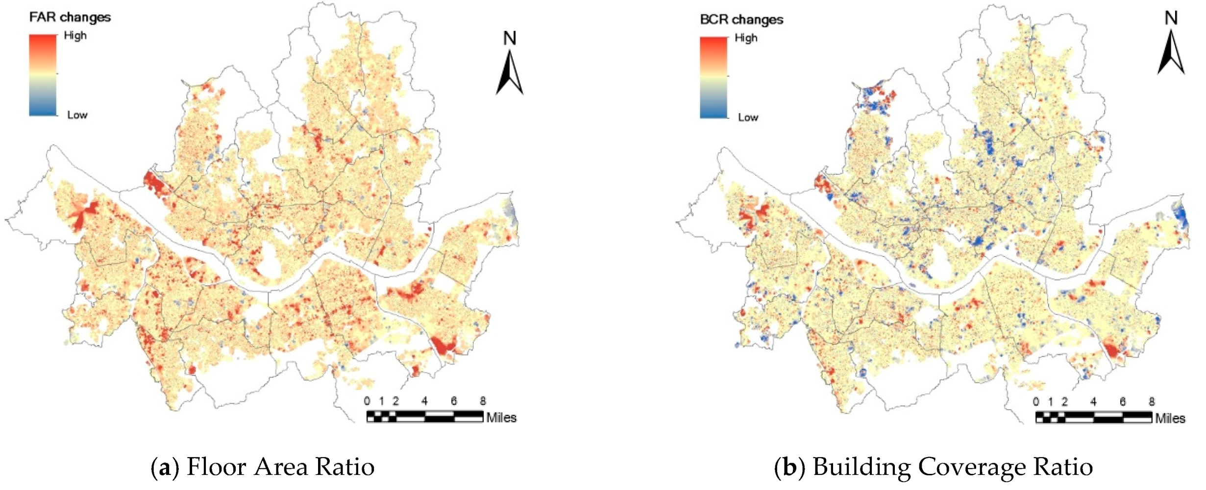
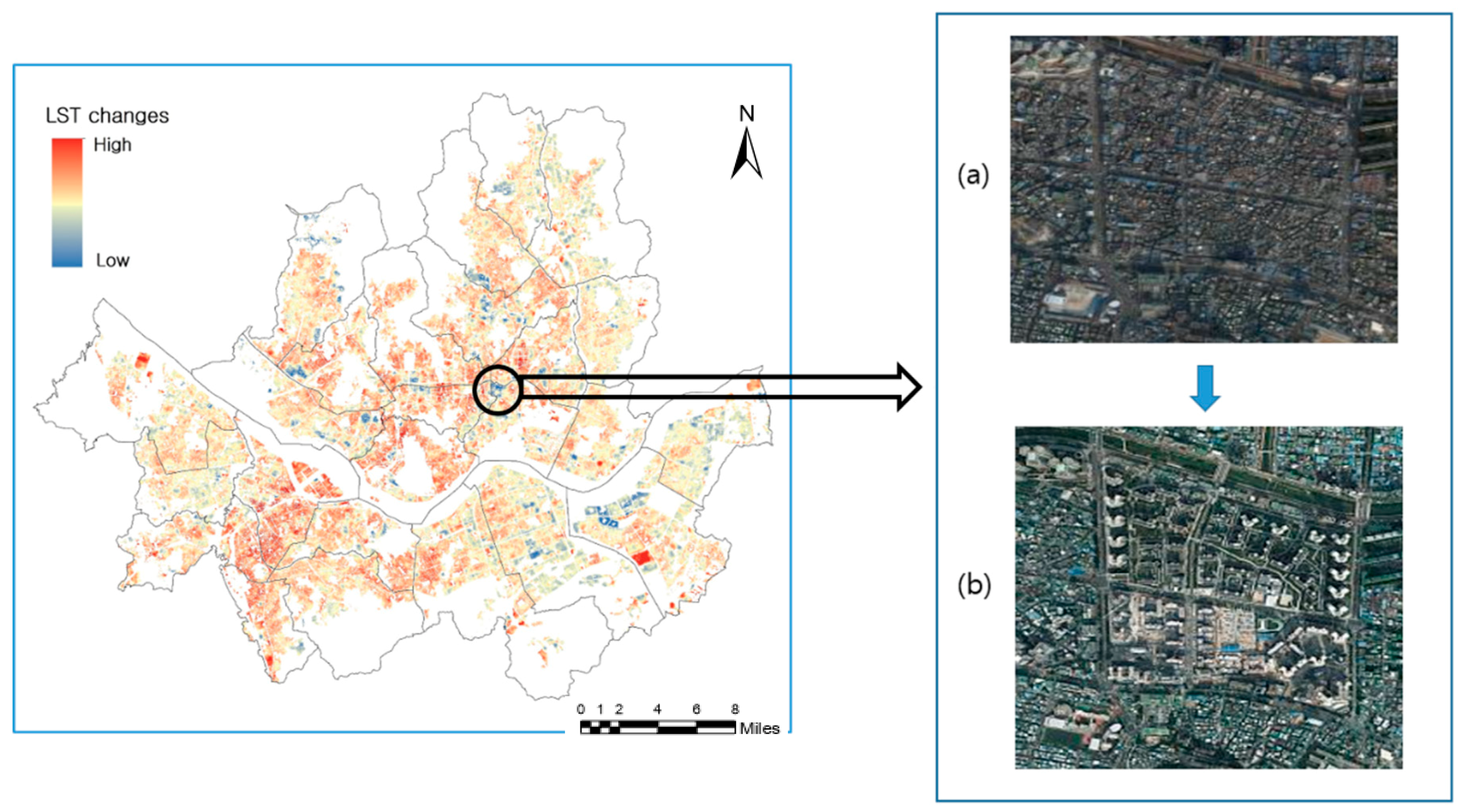
Our primary concern was the impact of urban land use on LST. Therefore, for our empirical analysis, we selected parcels for residential, commercial, and industrial use with 222,253 observations for each year. Table 2 presents the means and standard deviations for FAR, BCR, LST, and NDVI from the combined data set for 2004 and 2014. Maps (a)-(d) in Figure 1 show visual changes of the four measures, respectively. The figure illustrates that there seems to be a significant relationship between green areas and LST changes. In order to emphasize the relationship, an example of a zoom-in image was added in Figure 2. Figure 2 illustrates a redevelopment site that has experienced a significant LST reduction possibly due to residential densification from low-density (a) to high-density residential development (b).
Our data shows that the average ZLST in the study area decreased by 0.01 over the last decade, while the average NDVI increased by 0.09 during the same period, implying an increase in green vegetation and a slight decrease in ZLST. Increases in BCR and FAR over the last decade are also notable and indicate a greater building coverage ratio and higher density in 2014 than in 2004.
For the empirical analysis, we classified the urban land use parcels into six categories according to the FAR, as shown in Table 3. To protect the good living environment and designate areas that need to be in harmony with nearby residential and neighborhood living facilities, residential areas were subdivided into three residential areas depending on residential building heights: (1) Low-density residential area (R-1); (2) Medium-density residential area (R-2), and High-density residential areas (R-3).
The designation “semi-residential area” indicates the land for mixed residential and commercial use, while the “commercial area” designation includes central and general commercial areas as well as neighboring and circulating commercial areas as defined by the zoning ordinance. Semi-industrial area is the land for light industry or other industries, but needs supplementation of residential, commercial and business functions.
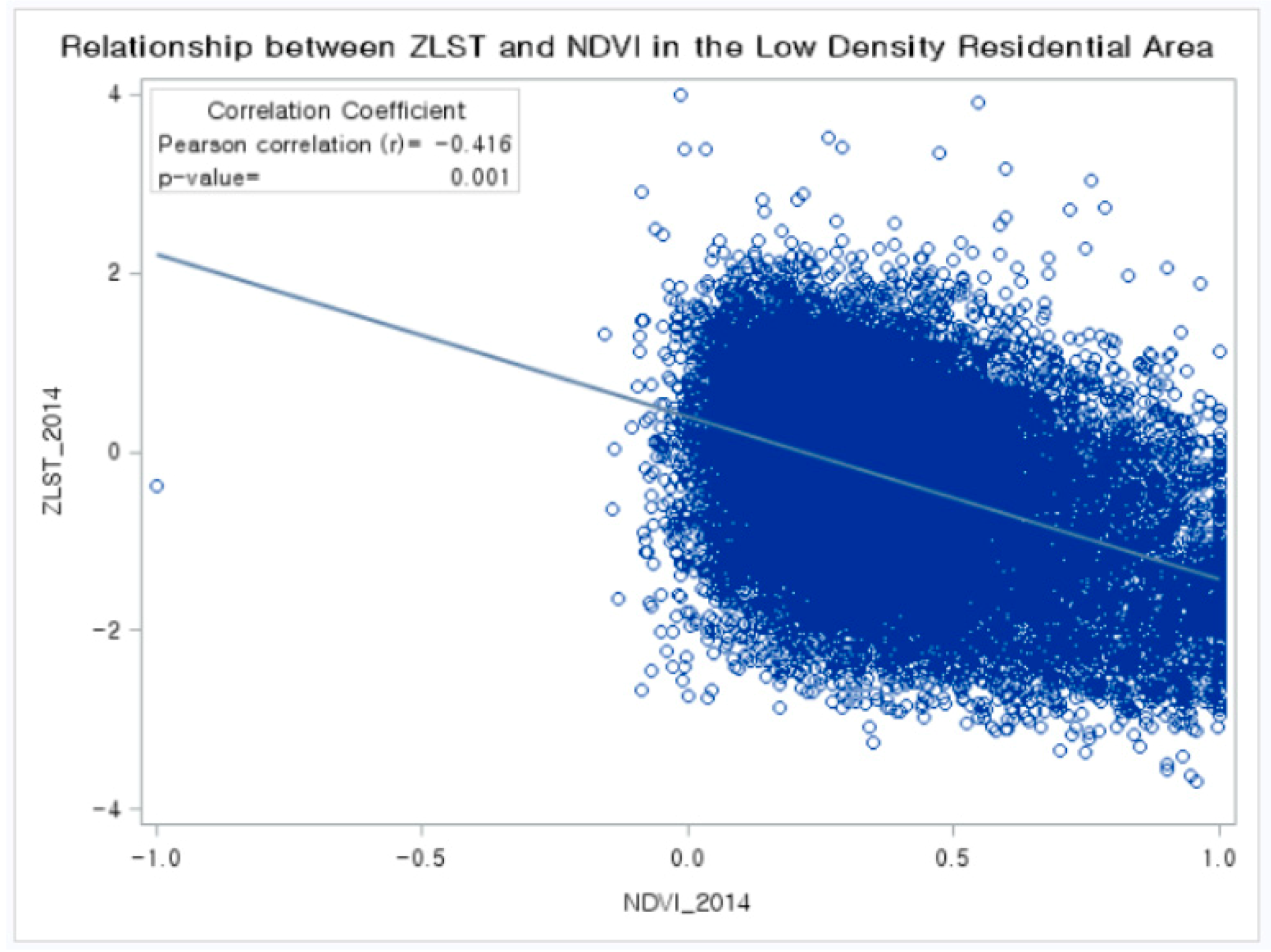
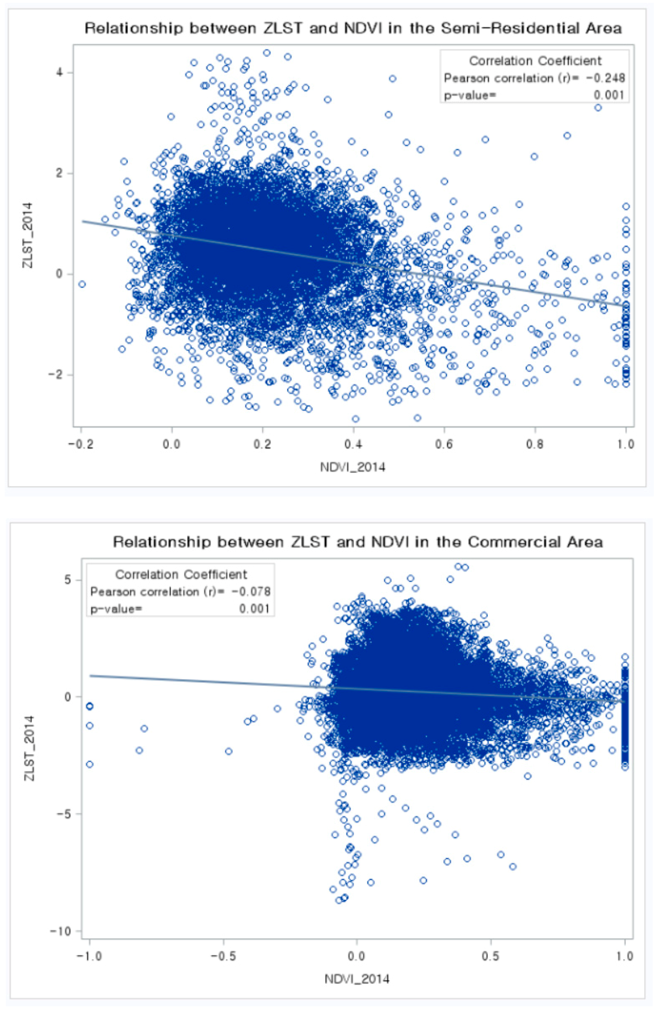
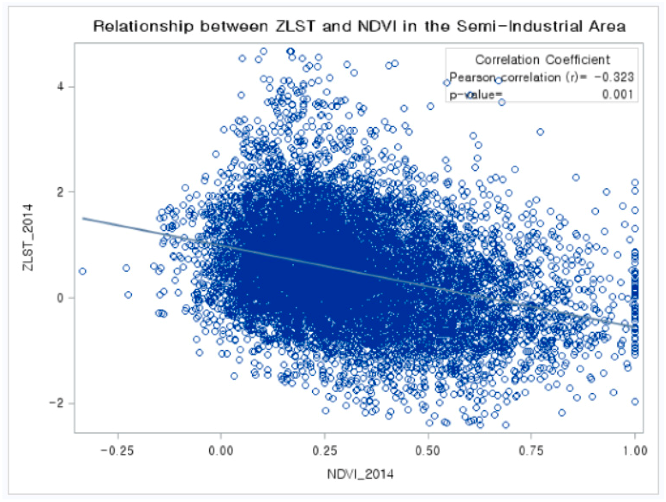
Table 4 presents changes in ZLST and NDVI by land use type between 2004 and 2014. The most significant ZLST change occurred in low-density and high-density residential areas between 2004 and 2014. In 2004, low-density residential areas had the lowest ZLST (−0.664), and high-density residential areas had the second lowest (−0.259). However, their order reverse in 2014 with the largest ZLST reduction in high-density residential areas (−0.156). On the other hand, low-density residential areas experienced the highest ZLST increase (0.367) during the 2004–2014 period. NDVI changes partly explained changes in ZLST caused by land use type. NDVI increases were found in land use types which experienced ZLST drops. This indicates a negative relationship between ZLST and NDVI. This argument is generally supported by Figure 3, showing that ZLST is negatively associated with NDVI for all of land use types at 1% significance level in terms of the Pearson correlation coefficient.
3.2. Statistical Analysis
To investigate the effects of land use type on LST, we built two pooled ordinary least squares (OLS) regression models by combining observations for both years, a base model, and a model with year dummy interaction variables. The pooled model can enhance statistical power and capture the interaction impacts between land use type and year on LST changes, while controlling for other factors affecting LST. For the base model, eight independent variables were used. They were NDVI, BCR, five land use type dummy variables (the low-density residential area is the reference group), and year dummy variable. served as the dependent variable. For the second model, we added five land use type interaction variables into the base model to capture the interaction impacts between land use type and year. As Jaccard and Turrisi [44] argued, it is possible to statistically test whether LST changes vary by land use type over time with the interaction variables that we used here.
Table 5 shows the OLS results for both models. The overall performance of the models is moderate with a R2 value of 0.28. All independent variables for both models were statistically significant (p < 0.01). The values of the variance inflation factor (VIF) ranged from 1.21 to 8.82, showing no serious collinearity with the exception of the year dummy variable in the second model (10.93).
Specific result are as follows. First, as we expected, the model results showed that the NDVI was negatively associated with LST and that BCR was positively associated with it; these findings indicate that larger BCR is likely to contribute to increasing LST. The base model results showed a positive coefficient value for the year dummy, implying that the LST in the study area has increased over the last decade after controlling other factors affecting LST.
Second, a notable finding is that the LSTs in all land use types were higher than the reference group (low-density residential areas), indicating that low-density residential areas have the lowest LST. Third, and most importantly, all the interaction variables had significant negative coefficient values in the second model. This finding indicates that LST has significantly reduced in dense land use areas during the 2004–2014 period, regardless of land use type, compared to LST change in low-density residential areas.
4. Conclusions and Implications
This study investigated how changes in LST were impacted by land use type, using Seoul as a case study. The descriptive analysis results showed that over a ten-year period, there was a rise in LST for low- and medium-density residential, and semi-industrial areas, whereas LST drops were found in high-density residential, semi-residential, and commercial areas. The multivariate statistical results partly supported these findings, yielding statistically significant negative coefficient values for all the interaction variables between higher-density land use types and the year dummy variable; this implies LST drops in higher-density land use areas. Our findings are consistent with studies of Stone et al. [8] and Chen et al. [45] who argue lower LSTs occur in compact urban areas in the United States and in city centers in China, respectively.
Our findings present several implications for urban planning and development. First, they offer empirical evidence for higher LST reduction in denser land uses, supporting the argument for compact development as a sustainable urban planning tool in terms of UHI effects. Since the land use classification in this study is based on zoning ordinances in Korea, the findings can help urban planners to understand the relationship between land use zoning and LST, and to develop land use planning measures for mitigating LST increases. Second, the larger LST reduction that occurred in higher- density areas appears to be related to residential densification in Seoul due to the provision of high-rise apartment complexes there. According to the SMG, the number of apartment complexes (The apartment complex is defined by number of building floors (5 or above) and apartment units (300 or more units)) in Seoul increased by 60.5% from 2652 in 2005 to 4256 in 2016, and the number of apartment buildings increased by 55.7% from 12,800 to 20,000 during the same period. In addition, more high-rise apartment buildings have been supplied between 2005 and 2016 with the increase in the share of 16 story or higher apartment buildings from 34.9% in 2005 to 38.3% in 2016 (http://data.seoul.go.kr/dataList/datasetView.do?infId=171&srvType=S&serviceKind=2: accessed 13 August 2018). The strong preference of higher-income residents for high-rise apartment buildings drove the increase in apartment supply because apartment complexes provide good amenities such as parks, walking paths, bike paths, convenient access to public transit, and safety by having gatekeepers.
Third, like many previous studies, our results also indicate that higher NDVI in denser land areas contributes to the LST reduction. This emphasizes the importance of providing green vegetation in the redevelopment or renovation process. In order to provide more green spaces to citizens, the SMG has implemented various park and green space policies under the 2030 park and green space master plan, including restoration of the Cheonggye stream in the downtown area, green rooftops, and open, green apartments with the removal of apartment complex walls. According to the SMG, parks and green spaces have increased from 284.5 square kilometers in 1999 to 318.2 square kilometers in 2014, representing a 12% increase (https://seoulsolution.kr/en/content/3497: accessed 14 August 2018.) Lastly, to the best of our knowledge, no previous studies have investigated the relationship between land use zoning and densification and LST. More empirical studies need to be conducted in other countries to elucidate this relationship and to find similarities and differences in that relationship through comparative studies.
Author Contributions
Conceptualization, J.-I.K. and M.-J.J.; data preparation, C.-H.Y.; formal analysis, K.-H.K., and J.Y.H.; writing—original draft preparation, M.-J.J.; writing—review and editing, J.-I.K.; supervision, J.-I.K.
Funding
This research received no external funding.
Conflicts of Interest
The authors declare no conflicts of interest.
References
- Oke, T.R. The energetic basis of the urban heat island. Q. J. R. Meteorol. Soc. 1982, 108, 1–24. [Google Scholar] [CrossRef]
- Oke, T.R. Boundary Layer Climates; Routledge: New York, NY, USA, 1987. [Google Scholar]
- Stone, B.; Rodgers, M. Urban form and thermal efficiency: How the design of cities influences the urban heat island effect. J. Am. Plan. Assoc. 2001, 67, 186–198. [Google Scholar] [CrossRef]
- Hondula, D.M.; Georgescu, M.; Balling, R.C. Challenges associated with projecting urbanization-induced heat-related mortality. Sci. Total Environ. 2014, 490, 538–544. [Google Scholar] [CrossRef] [PubMed]
- EPA (US Environmental Protection Agency). Heat Island Impacts; United States Environmental Protection Agency: Washington, DC, USA, 2016. Available online: http://www.epa.gov/hiri/impacts/index.htm (accessed on 23 August 2018).
- Whitman, S.; Good, G.; Donoghue, E.R.; Benbow, N.; Shou, W.; Mou, S. Mortality in Chicago attributed to the July 1995 heat wave. Am. J. Public Health 1997, 87, 1515–1518. [Google Scholar] [CrossRef] [PubMed] [Green Version]
- Robine, J.M.; Cheung, S.L.K.; Le Roy, S.; Van Oyen, H.; Griffiths, C.; Michel, J.P.; Herrmann, F.R. Death toll exceeded 70,000 in Europe during the summer of 2003. Comptes Rendus Biol. 2008, 331, 171–178. [Google Scholar] [CrossRef] [PubMed]
- Stone, B.; Hess, J.; Frumkin, H. Urban form and extreme heat events: Are sprawling cities more vulnerable to climate change than compact cities? Environ. Health Perspect. 2010, 118, 1425–1428. Available online: http://users.metu.edu.tr/ioguz/Stone_2010.pdf (accessed on 22 February 2016). [CrossRef] [Green Version]
- Gago, E.J.; Roldán, J.; Pacheco-Torres, R.; Ordóñez, J. The city and urban heat islands: A review of strategies to mitigate adverse effects. Renew. Sustain. Energy Rev. 2013, 25, 749–758. [Google Scholar] [CrossRef]
- Deilami, K.; Kamruzzamanb, M.D.; Liu, Y. Urban heat island effect: A systematic review of spatio-temporal factors, data, methods, and mitigation measures. Int. J. Appl. Earth Obs. Geoinfor. 2018, 67, 30–42. [Google Scholar] [CrossRef]
- Wang, S.; Ma, Q.; Ding, H.; Liang, H. Detection of urban expansion and land surface temperature change using multi-temporal Landsat images. Resour. Conserv. Recycl. 2018, 128, 526–534. [Google Scholar] [CrossRef]
- Weng, Q.; Liu, H.; Lu, D. Assessing the effects of land use and land cover patterns on thermal conditions using landscape metrics in city of Indianapolis, United States. Urban Ecosyst. 2007, 10, 203–219. [Google Scholar] [CrossRef]
- Xiao, H.; Weng, Q. The impact of land use and land cover changes on land surface temperature in a karst area of China. J. Environ. Manag. 2007, 85, 245–257. [Google Scholar] [CrossRef] [PubMed]
- Thi Van, T.; Xuan Bao, H.A. Study of the impact of urban development on surface temperature using remote sensing in Ho Chi Minh City. South. Vietnam. Geogr. Res. 2010, 48, 86–96. [Google Scholar]
- Rinner, C.; Hussain, M. Toronto’s urban heat island-exploring the relationship between land use and surface temperature. Remote Sens. 2011, 3, 1251–1265. [Google Scholar] [CrossRef] [Green Version]
- Balçik, F. Determining the impact of urban components on land surface temperature of Istanbul by using remote sensing indices. Environ. Monit. Assess. 2014, 186, 859–872. [Google Scholar] [CrossRef] [PubMed]
- Heusinkveld, B.G.; Steeneveld, G.J.; Hove, L.V.; Jacobs, C.M.J.; Holtslag, A.A.M. Spatial variability of the Rotterdam urban heat island as influenced by urban land use. J. Geophys. Res. Atmos. 2014, 119, 677–692. [Google Scholar] [CrossRef]
- Buyadi, S.; Mohd, W.; Misni, A. Impact of land use changes on the surface temperature distribution of area surrounding the National Botanic Garden, Shah Alam. Soc. Behav. Sci. 2013, 101, 516–525. [Google Scholar] [CrossRef] [Green Version]
- Emmanuel, R.; Loconsole, A. Green infrastructure as an adaptation approach to tackling urban overheating in the Glasgow Clyde Valley Region, UK. Landsc. Urban Plan. 2015, 138, 71–86. [Google Scholar] [CrossRef] [Green Version]
- Quan, J.; Zhan, W.; Chen, Y.; Wang, M.; Wang, J. Time series decomposition of remotely sensed land surface temperature and investigation of trends and seasonal variations in surface urban heat islands. J. Geophys. Res. Atmos. 2016, 121, 2638–2657. [Google Scholar]
- EPA (US Environmental Protection Agency). Reducing Urban Heat Islands: Compendium of Strategies; US Environmental Protection Agency: Washington, DC, USA, 2008.
- Zhou, W.; Huang, G.; Cadenasso, M.L. Does spatial configuration matter? Understanding the effects of land cover pattern on land surface temperature in urban landscapes. Landsc. Urban Plan. 2011, 102, 54–63. [Google Scholar] [CrossRef]
- Li, X.; Zhou, W.; Ouyang, Z.; Xu, W.; Zheng, H. Spatial pattern of green space affects land surface temperature: Evidence from the heavily urbanized Beijing metropolitan area, China. Landsc. Ecol. 2012, 27, 887–898. [Google Scholar] [CrossRef]
- Qwen, T.W.; Carlson, T.N.; Gilles, R.R. An assessment of satellite remotely sensed land cover parameters in quantitatively describing the climatic effect of urbanization. Int. J. Remote Sens. 1998, 19, 1663–1681. [Google Scholar]
- Yuan, F.; Wu, C.; Bauer, M.E. Comparison of impervious surface area and normalized difference vegetation index as indicators of surface urban heat island effects in Landsat imagery. Remote Sens. Environ. 2007, 106, 375–386. [Google Scholar] [CrossRef]
- Bokaie, M.; Zarkesh, M.K.; Arasteh, P.D.; Hosseini, A. Assessment of urban heat island based on the relationship between land surface temperature and land use/land cover in Tehran. Sustain. Cities Soc. 2016, 23, 94–104. [Google Scholar] [CrossRef]
- Jun, M.; Kim, J.; Kim, H.; Yeo, C.; Hyun, J. Effects of two urban development strategies on changes in the land surface temperature: Infill versus suburban new town development. J. Urban Plan. Dev. 2017, 143, 04017010. [Google Scholar] [CrossRef]
- Stone, B.; Norman, J. Land use planning and surface heat island formation: A parcel-based radiation flux approach. Atmos. Environ. 2006, 40, 3561–3573. [Google Scholar] [CrossRef]
- Schwarz, N.; Manceur, A. Analyzing the influence of urban forms on surface urban heat islands in Europe. J. Urban Plan. Dev. 2015, 141, A4014003. [Google Scholar] [CrossRef]
- Benas, N.; Chrysoulakis, N.; Cartalis, C. Trends of urban surface temperature and heat island characteristics in the Mediterranean. Theor. Appl. Climatol. 2016, 130, 807–816. [Google Scholar] [CrossRef]
- Song, C.; Woodcock, C.E.; Seto, K.C.; Lenney, M.P.; Macomber, S.A. Classification and change detection using Landsat TM data: When and how to correct atmospheric effects? Remote Sens. Environ. 2001, 75, 230–244. [Google Scholar] [CrossRef]
- Sobrino, J.A.; Jiménez-Muñoz, J.C.; Paolini, L. Land surface temperature retrieval from LANDSAT TM 5. Remote Sens. Environ. 2004, 90, 434–440. [Google Scholar] [CrossRef]
- Mutiibwa, D.; Strachan, S.; Albright, T. Land surface temperature and surface air temperature in complex terrain. IEEE J. Sel. Top. Appl. Earth Obs. Remote Sens. 2015, 8, 4762–4774. [Google Scholar] [CrossRef]
- Bonafoni, S. Downscaling of Landsat and MODIS Land Surface Temperature Over the Heterogeneous Urban Area of Milan. IEEE J. Sel. Top. Appl. Earth Obs. Remote Sens. 2016, 9, 2019–2027. [Google Scholar] [CrossRef]
- Gerace, A.; Montanaro, M. Derivation and validation of the stray light correction algorithm for the thermal infrared sensor onboard Landsat 8. Remote Sens. Environ. 2017, 191, 246–257. [Google Scholar] [CrossRef]
- Qin, Z.; Kamieli, A.; Berliner, P. A mono-window algorithm for retrieving land surface temperature from Landsat TM data and its application to the Israel-Egypt border region. Int. J. Remote Sens. 2001, 22, 3719–3746. [Google Scholar] [CrossRef]
- Zhi-Hao, Q.; Zhang, M.H.; Karnieli, A. Mono-window algorithm for retrieving land surface temperature from Landsat TM6 data. ACTA Geogr. Sin. Chin. Ed. 2001, 56, 466–474. [Google Scholar]
- Jiménez-Muñoz, J.; Sobrino, J. A generalized single-channel method for retrieving land surface temperature from remote sensing data. J. Geophys. Res. 2003, 108. [Google Scholar] [CrossRef] [Green Version]
- Jiménez-Muñoz, J.; Cristobal, J.; Sobrino, J.; Soria, G.; Ninyerola, M.; Pons, X. Revision of the single-channel algorithm for land surface retrieval from Landsat thermal-infrared data. IEEE Trans.Geosci. Remote Sens. 2009, 47, 339–349. [Google Scholar] [CrossRef]
- Gillespie, A.; Rokugawa, S.; Matsunaga, T.; Cothern, J.S.; Hook, S.; Kahle, A.B. A temperature and emissivity separation algorithm for Advanced Spaceborne Thermal Emission and Reflection Radiometer (ASTER) images. IEEE Trans. Geosci. Remote Sens. 1998, 36, 1113–1126. [Google Scholar] [CrossRef]
- Liu, L.; Zhang, Y. Urban heat island analysis using the Landsat TM data and ASTER data: A case study in Hong Kong. Remote Sens. 2011, 3, 1535–1552. [Google Scholar] [CrossRef] [Green Version]
- Sospedra, F.; Caselles, V.; Valor, E. Effective wavenumber for thermal infrared bands-application to Landsat-TM. Int. J. Remote Sens. 1998, 19, 2105–2117. [Google Scholar] [CrossRef]
- Rogan, J.; Ziemer, M.; Martin, D.; Ratick, S.; Cuba, N.; DeLauer, V. The impact of tree cover loss on land surface temperature: A case study of central Massachusetts using Landsat Thematic Mapper thermal data. App. Geogr. 2013, 45, 49–57. [Google Scholar] [CrossRef]
- Jaccard, J.; Turrisi, R. Interaction Effects in Multiple Regression, 2nd ed.; Sage University Papers Series on Quantitative Applications in the Social Sciences, 07-072; Sage: Thousand Oaks, CA, USA, 2003. [Google Scholar]
- Chen, L.; Jiang, R.; Xiang, W. Surface heat island in Shanghai and its relationship with urban development from 1989 to 2013. Adv. Meteorol. 2016, 2016, 9782686. [Google Scholar] [CrossRef]
Figure 1.
Changes of FAR, BCR, LST, and NDVI: 2004–2014 (Latitude longitude coordinates for Seoul are 37°33′57.6′’ N, 126°58′42.24′’ E).
Figure 1.
Changes of FAR, BCR, LST, and NDVI: 2004–2014 (Latitude longitude coordinates for Seoul are 37°33′57.6′’ N, 126°58′42.24′’ E).


Figure 2.
An example of redevelopment site having a significant LST reduction due to densification: (a) single-family housing units in 2008, (b) apartment complexes in 2014. The figure (a) and (b) are captured from Google images (Latitude longitude coordinates for Seoul are 37°33′57.6′′ N, 126°58′42.24′′ E).

Figure 3.
The relationship between ZLST and NDVI by land use type in 2014.


Table 1.
Basic information on the satellite images for 2004 and 2014.
| Attribute | 2004 | 2014 |
|---|---|---|
| Satellite Image | Landsat TM 5 | Landsat 8 |
| Sensor | TM | OLI TIRS |
| Date/Time Acquired | June 3/13:52 | September 19/14:11 |
| Projection/Datum | UTM zone52/WGS84 | UTM zone52/WGS84 |
| Number of Bands | 7 | 11 |
| Thermal Band | 6 | 10, 11 |
| Red Band/NIR Band | 3/4 | 4/5 |
Source: Jun et al. (2017) [27].
Table 2.
Summary statistics for parcels for residential, commercial, and industrial use.
| 2004 | 2014 | |||
|---|---|---|---|---|
| Mean | S.D. | Mean | S.D. | |
| Z-scored land surface temperature (ZLST) | 0.024 | 0.987 | 0.013 | 0.997 |
| Normalized difference vegetation index (NDVI) | 0.211 | 0.108 | 0.302 | 0.203 |
| Building coverage ratio (BCR) | 0.403 | 0.131 | 0.410 | 0.130 |
| Floor area ratio (FAR) | 1.950 | 1.172 | 2.126 | 1.282 |
| N | 222,253 | 222,253 | ||
Table 3.
Land use classification and FAR in Korean zoning ordinance.
| Land Use Classification | Floor Area Ratio (FAR), % |
|---|---|
| Low-density residential area | 50–200 |
| Medium-density residential area | 150–250 |
| High-density residential area | 200–300 |
| Semi-residential area | 200–500 |
| Commercial area | 200–1500 |
| Semi-industrial area | 200–400 |
Table 4.
Changes in ZLST and NDVI by land use type between 2004 and 2014.
| Land Use Types | Share * | 2004 | 2014 | Difference between 2004 and 2014 | |||
|---|---|---|---|---|---|---|---|
| ZLST | NDVI | ZLST | NDVI | ZLST | NDVI | ||
| Low-density residential areas | 9.2% | −0.664 | 0.296 | −0.297 | 0.381 | 0.367 | 0.084 |
| Medium-density residential areas | 42.7% | 0.243 | 0.188 | 0.271 | 0.249 | 0.028 | 0.062 |
| High-density residential areas | 32.0% | −0.259 | 0.238 | −0.415 | 0.379 | −0.156 | 0.141 |
| Semi-residential areas | 3.9% | 0.513 | 0.161 | 0.459 | 0.215 | −0.054 | 0.054 |
| Commercial areas | 7.5% | 0.265 | 0.166 | 0.237 | 0.214 | −0.028 | 0.048 |
| Semi-industrial areas | 4.7% | 0.508 | 0.191 | 0.511 | 0.309 | 0.003 | 0.118 |
* The share of total number of parcels (444,506) used in the analysis.
Table 5.
Pooled OLS results.
| Variables | Base Model | Model with Interaction Variables | ||||
|---|---|---|---|---|---|---|
| β | t-Value | VIF | β | t-Value | VIF | |
| Intercept | −0.506 | −74.9 *** | 0.00 | −0.681 | −87.3 *** | 0.00 |
| NDVI | −1.912 | −222.7 *** | 1.32 | −1.911 | −221.4 *** | 1.34 |
| BCR | 1.633 | 153.3 *** | 1.21 | 1.630 | 153.3 *** | 1.21 |
| Medium-density residential areas | 0.394 | 83.7 *** | 3.40 | 0.579 | 88.9 *** | 6.55 |
| High-density residential areas | 0.087 | 18.3 *** | 3.05 | 0.285 | 42.9 *** | 6.07 |
| Semi-residential areas | 0.537 | 69.1 *** | 1.41 | 0.774 | 70.8 *** | 2.80 |
| Commercial areas | 0.279 | 43.9 *** | 1.77 | 0.510 | 57.9 *** | 3.42 |
| Semi-industrial areas | 0.795 | 110.3 *** | 1.45 | 0.949 | 94.4 *** | 2.84 |
| Year | 0.153 | 57.6 *** | 1.10 | 0.508 | 61.1 *** | 10.93 |
| Medium-density residential area x Year | - | - | - | −0.374 | −40.9 *** | 8.82 |
| High-density residential area x Year | - | - | - | −0.401 | −42.5 *** | 7.58 |
| Semi-residential area x Year | - | - | - | −0.476 | −31.2 *** | 2.85 |
| Commercial area x Year | - | - | - | −0.465 | −37.6 *** | 3.50 |
| Semi-industrial area x Year | - | - | - | −0.312 | −21.8 *** | 2.88 |
| N | 444,506 | 444,506 | ||||
| Adjusted R2 | 0.281 | 0.284 | ||||
Notes: (1) *** p < 0.01; (2) The reference variable is low-density residential use.
© 2019 by the authors. Licensee MDPI, Basel, Switzerland. This article is an open access article distributed under the terms and conditions of the Creative Commons Attribution (CC BY) license (http://creativecommons.org/licenses/by/4.0/).
Share and Cite
MDPI and ACS Style
Kim, J.-I.; Jun, M.-J.; Yeo, C.-H.; Kwon, K.-H.; Hyun, J.Y. The Effects of Land Use Zoning and Densification on Changes in Land Surface Temperature in Seoul. Sustainability 2019, 11, 7056. https://doi.org/10.3390/su11247056
AMA Style
Kim J-I, Jun M-J, Yeo C-H, Kwon K-H, Hyun JY. The Effects of Land Use Zoning and Densification on Changes in Land Surface Temperature in Seoul. Sustainability. 2019; 11(24):7056. https://doi.org/10.3390/su11247056
Chicago/Turabian StyleKim, Jae-Ik, Myung-Jin Jun, Chang-Hwan Yeo, Ki-Hyun Kwon, and Jun Yong Hyun. 2019. "The Effects of Land Use Zoning and Densification on Changes in Land Surface Temperature in Seoul" Sustainability 11, no. 24: 7056. https://doi.org/10.3390/su11247056
Note that from the first issue of 2016, this journal uses article numbers instead of page numbers. See further details here.