Grocery Delivery or Customer Pickup—Influences on Energy Consumption and CO2 Emissions in Munich


Abstract
:1. Introduction
- An assessment methodology for the investigation of energy and CO2 savings as well as break-even points based on real-world geodata derived from OpenStreetMap and Monte Carlo simulations is presented
- The use of electric vehicles for the delivery of groceries
- Break-even points for energy and carbon dioxide emissions
- Impact evaluation of electric and combustion-engine private vehicle fleets for customer pickup trips on possible savings
- Evaluation of two different amounts of delivered customers
- Results analysis for a district of Munich, Germany
2. Materials and Methods
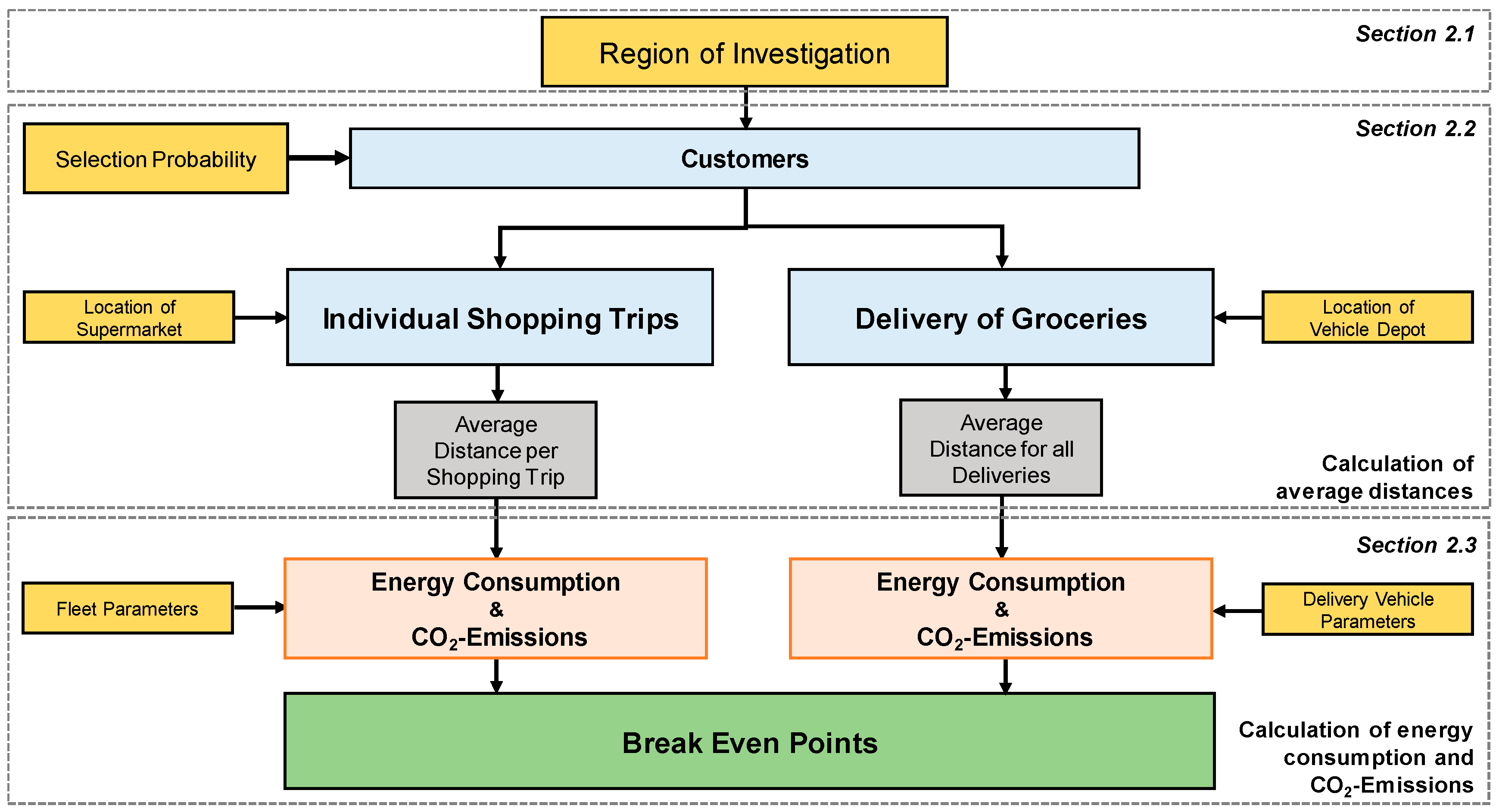
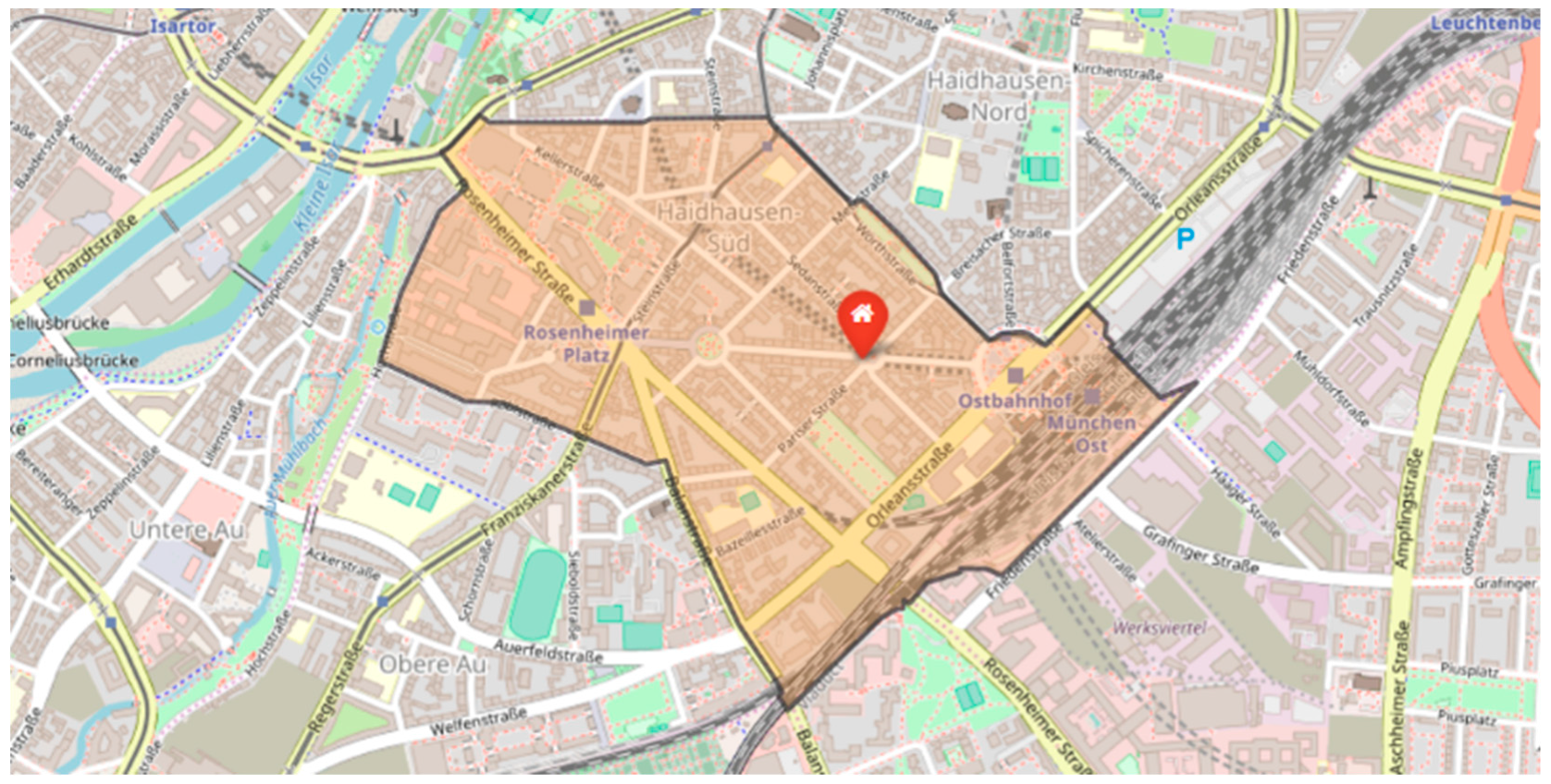
2.1. Region of Investigation
2.2. Calculation of Average Distances
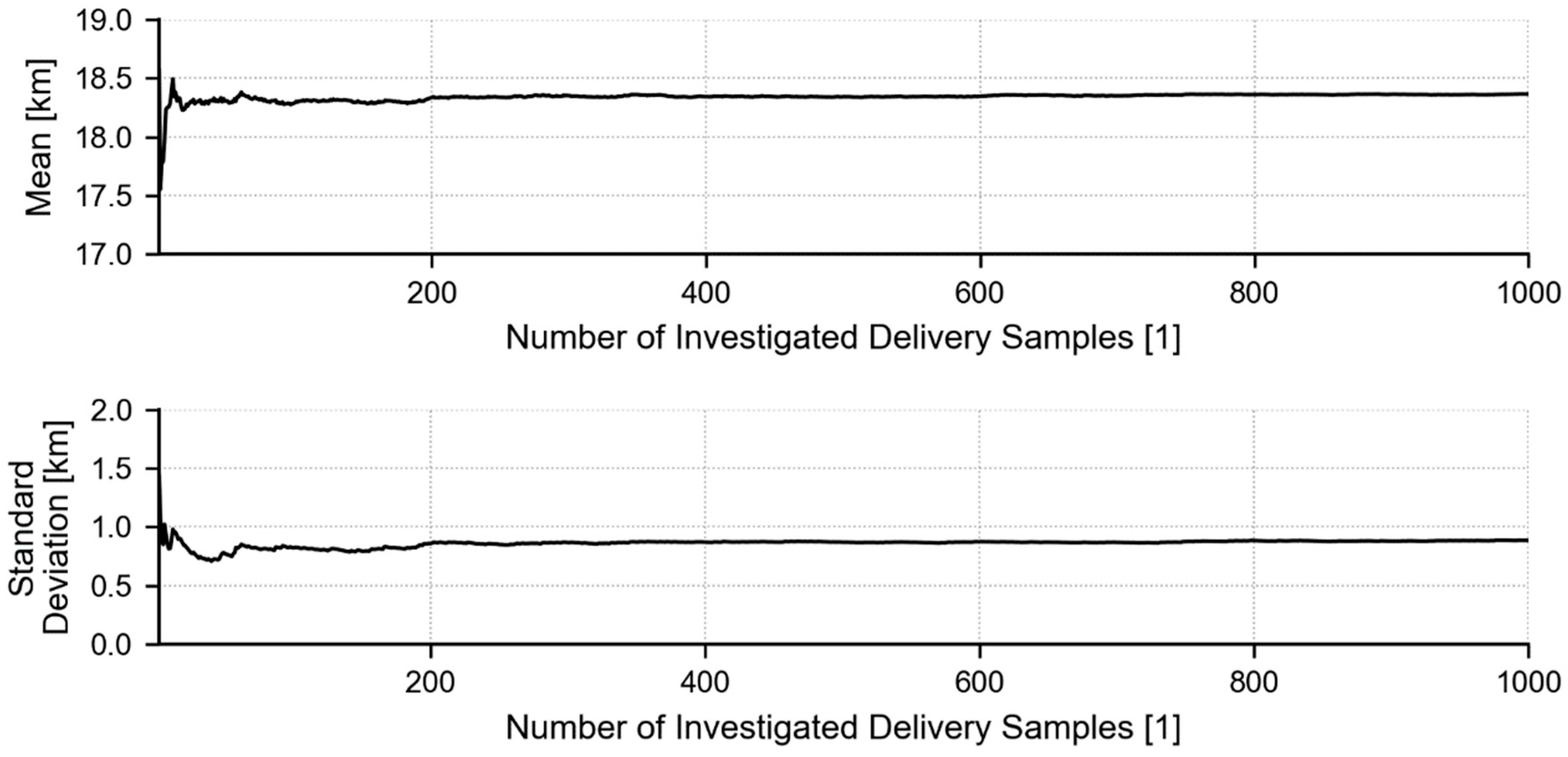
2.2.1. Creation of Delivery Samples
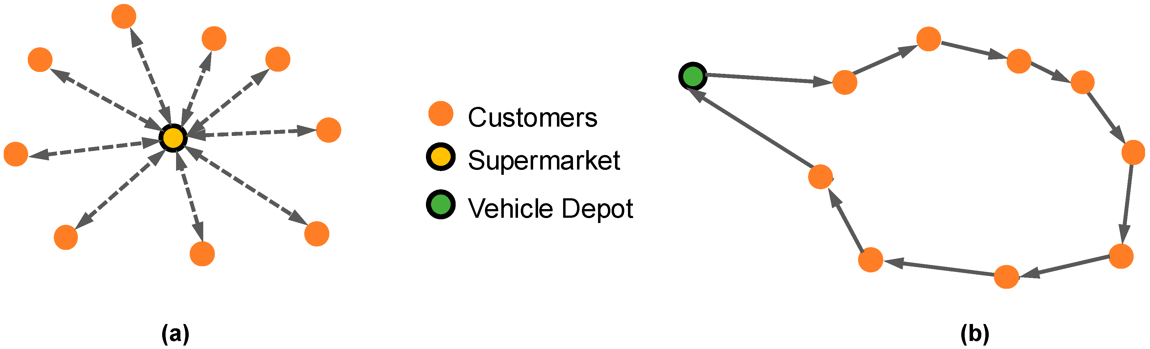
2.2.2. Tours of Delivery Vehicles
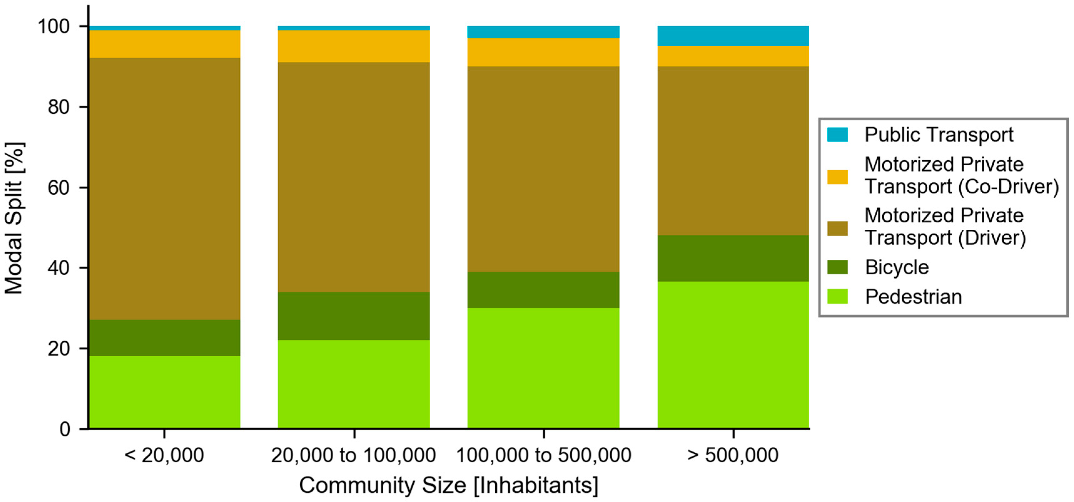
2.2.3. Customers Shopping Trips
2.3. Energy Consumption and Emission Factors
2.3.1. Delivery Vehicle Fleet
- represents the empty mass of the vehicle, including the driver and all necessary components for operating the vehicle (for example fuel, lubricants etc.)
- reflects the load mass of the vehicle, i.e., the mass of the delivered groceries.
- BPDC is representative for delivery vehicles in Haidhausen Süd
- Velocity and acceleration are not affected by different drive technologies of the vehicles, i.e., values of acceleration and deceleration are equal for all investigated vehicles.
2.3.2. Customer Vehicle Fleet
2.3.3. Calculation of Break-Even-Points
3. Results and Discussion
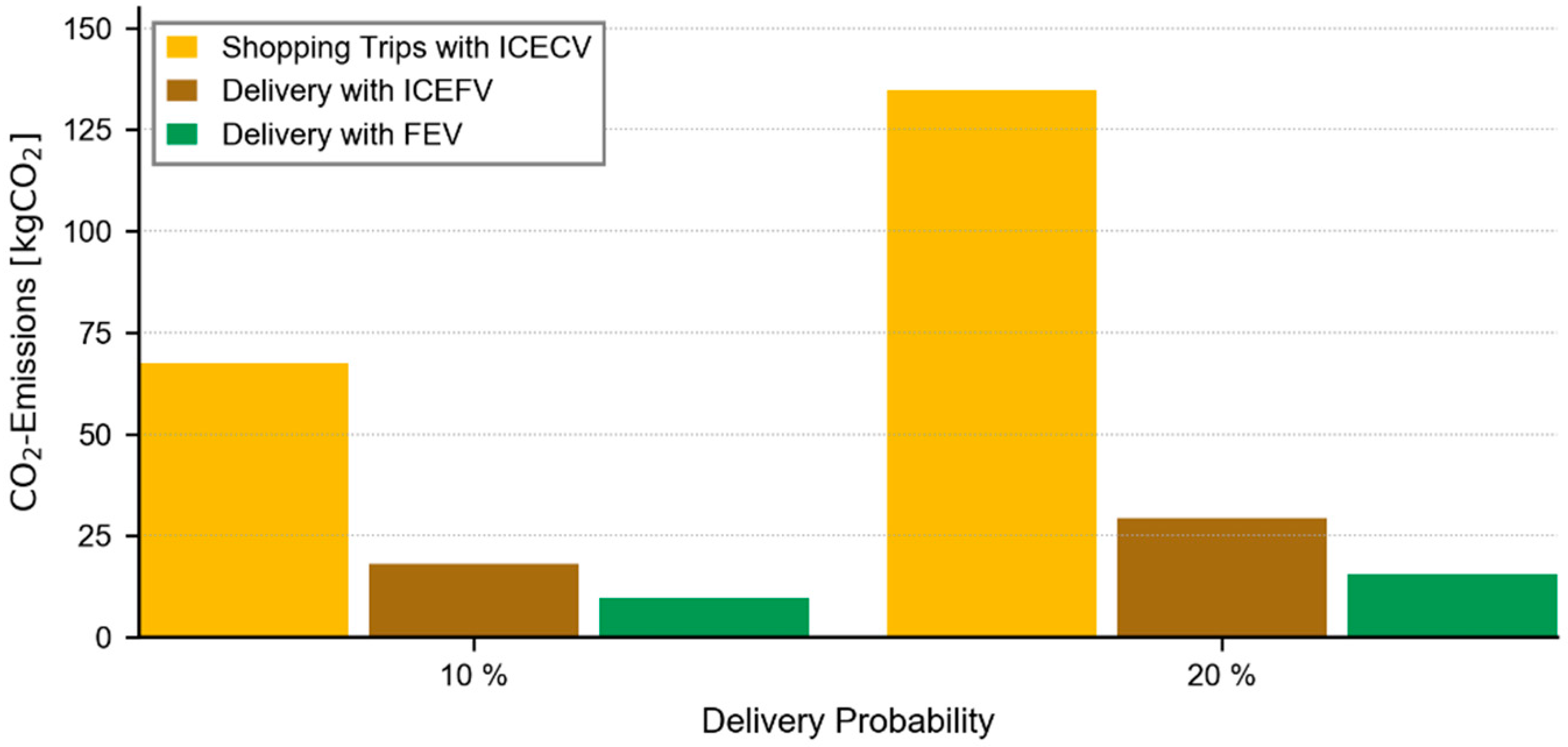
3.1. Potential for Saving of Energy and CO2 at the Current Share of Private Vehicle Use for Shopping Trips
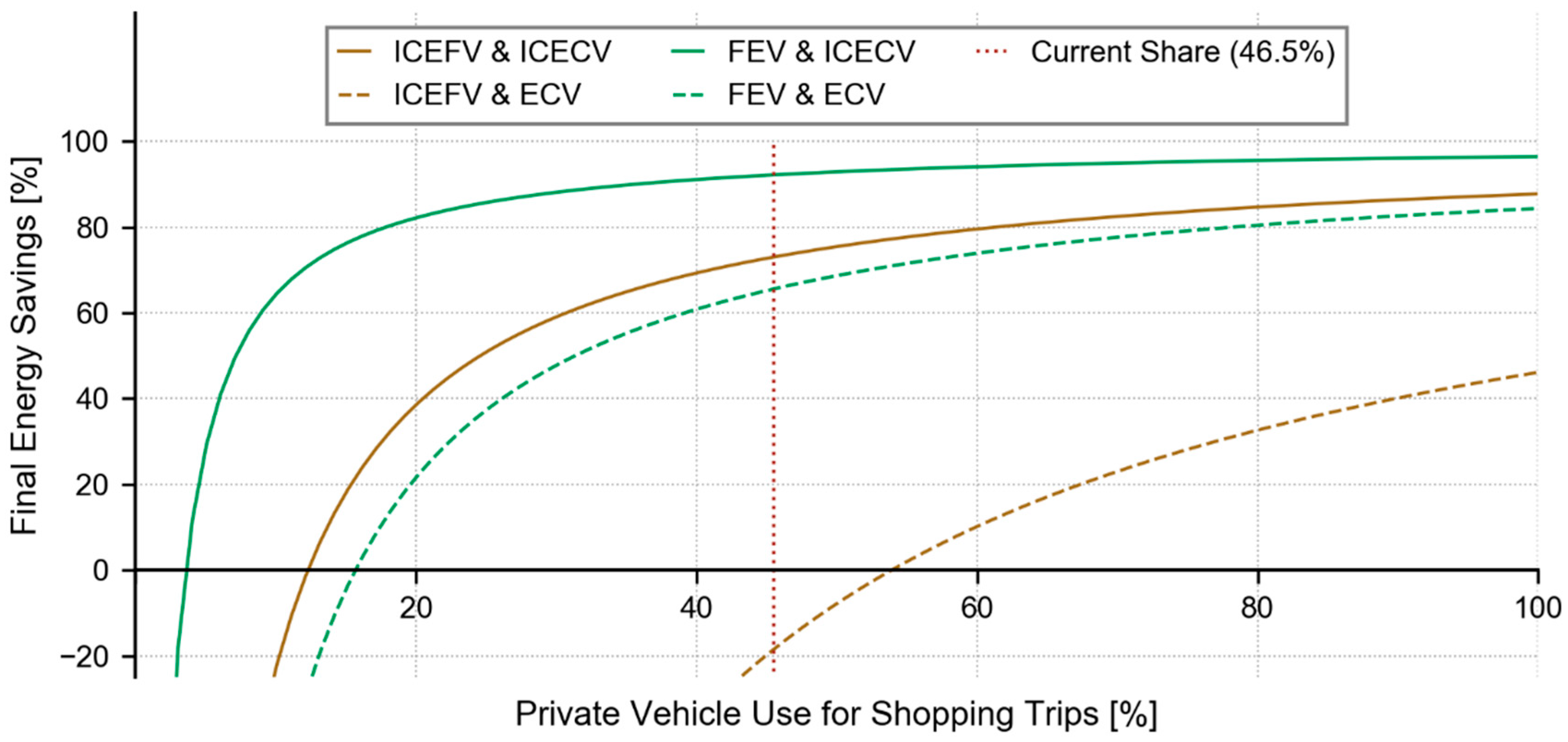
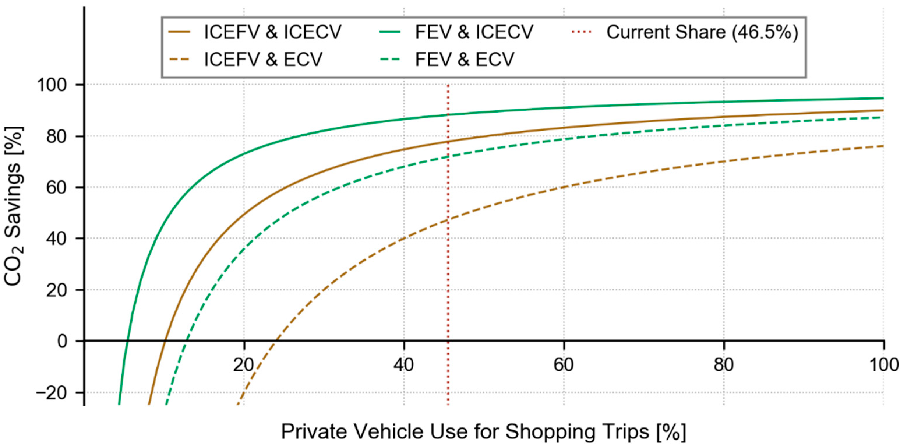
3.2. Analysis of Break-Even Points for Energy Consumption
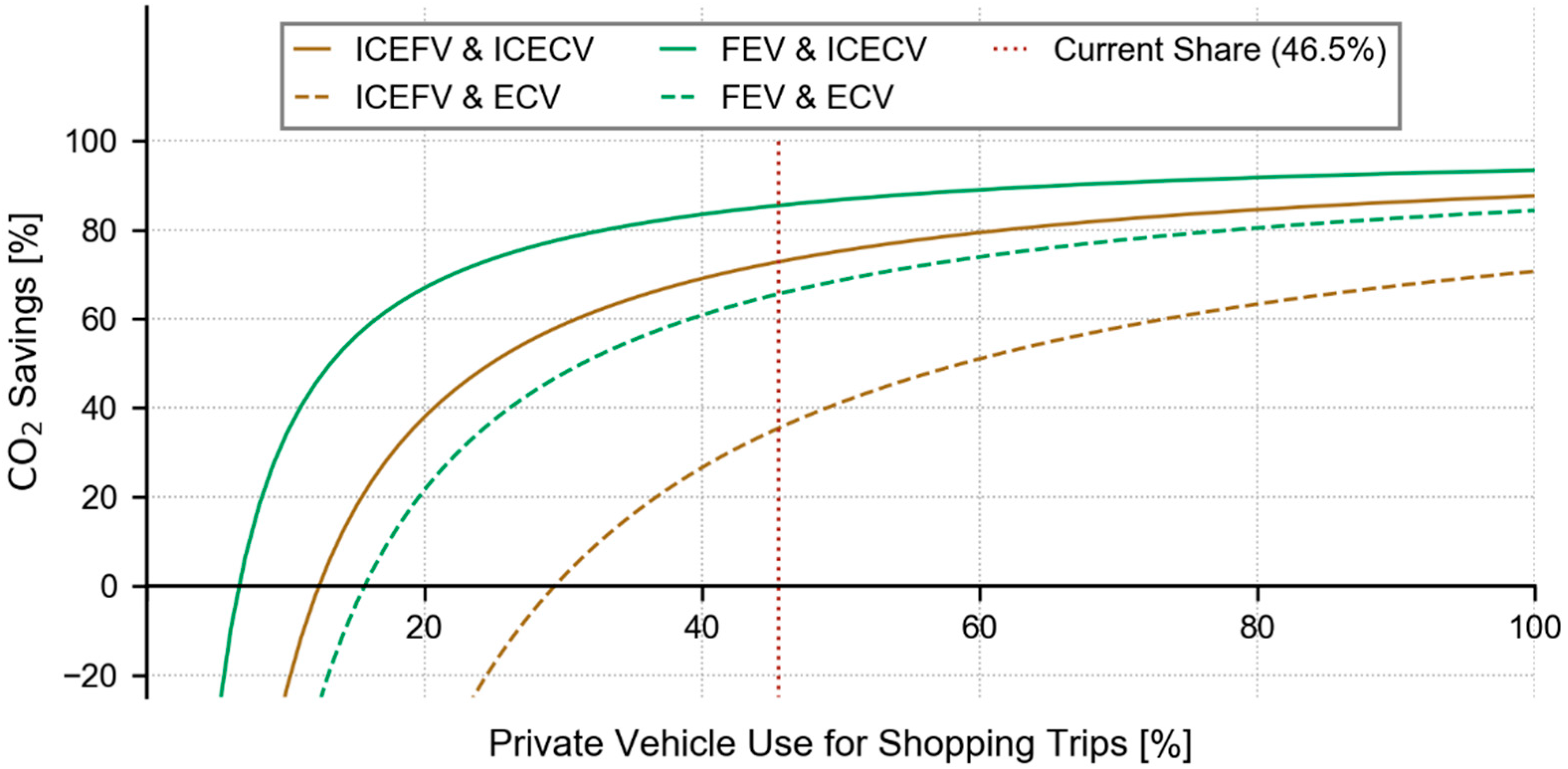
3.3. Analysis of Break-Even Points for CO2 Emissions
4. Conclusions and Outlook
- Specific energy consumption and specific CO2 emissions of private as well as delivery vehicles clearly affect the position of break-even points
- Break-even points for energy use and carbon dioxide emissions must be evaluated independently of each other, because the results can differ
- When internal combustion-engine delivery vehicles are used, a complete electrification of the private vehicle fleet can cause additional energy consumption at the current share of private vehicle use for shopping trips in Germany
- In this case, a reduction of the specific CO2 emissions of the electricity mix could also lead to additional emissions caused by the delivery
- At the current share of private vehicle use, an electrification of the private vehicle fleet requires the use of electric delivery vehicles in the future if energy savings and emission reductions are still to be made
- The trips of the customers start and end at the same positions. Chained customer shopping trips are not considered. The integration of the grocery purchase in other trips (for example in the trip to return from work) leads to a shift of the break-even points as the distances of customer trips decrease. Hence, more customers can use the private vehicle for grocery shopping to reach the energy consumption and CO2 emissions of the delivery vehicles.
- Time windows for delivery are not considered in the optimization of the route; the integration of this approach would also lead to a shift of the break-even points, since the distance covered by the delivery vehicles changes. In addition to that, perhaps more delivery vehicles must be employed.
- The refrigeration of the stowage of the delivery vehicles is not considered; a consideration would lead to higher specific energy consumption, resulting in a shift of the break-even points.
Author Contributions
Funding
Conflicts of Interest
References
- Bundesministerium für Verkehr und digitale Infrastruktur (BMVI). Verkehr in Zahlen 2017/2018: 46. Jahrgang: Berlin, Germany, 2017. Available online: https://www.bmvi.de/SharedDocs/DE/Publikationen/G/verkehr-in-zahlen-pdf-2017-2018.pdf (accessed on 21 January 2019).
- Siikavirta, H.; Punakivi, M.; Kärkkäinen, M.; Linnanen, L. Effects of E-Commerce on Greenhouse Gas Emissions: A Case Study of Grocery Home Delivery in Finland. J. Ind. Ecol. 2002, 6, 83–97. [Google Scholar] [CrossRef]
- Halldórsson, Á.; Edwards, J.B.; McKinnon, A.C.; Cullinane, S.L. Comparative analysis of the carbon footprints of conventional and online retailing. Int. J. Phys Distrib. Logist. Manag. 2010, 40, 103–123. [Google Scholar] [CrossRef]
- Wehner, J. Energy Efficiency in Logistics: An Interactive Approach to Capacity Utilisation. Sustainability 2018, 10, 1727. [Google Scholar] [CrossRef]
- Ranieri, L.; Digiesi, S.; Silvestri, B.; Roccotelli, M. A Review of Last Mile Logistics Innovations in an Externalities Cost Reduction Vision. Sustainability 2018, 10, 782. [Google Scholar] [CrossRef]
- Kin, B.; Ambra, T.; Verlinde, S.; Macharis, C. Tackling Fragmented Last Mile Deliveries to Nanostores by Utilizing Spare Transportation Capacity—A Simulation Study. Sustainability 2018, 10, 653. [Google Scholar] [CrossRef]
- Bányai, T. Real-Time Decision Making in First Mile and Last Mile Logistics: How Smart Scheduling Affects Energy Efficiency of Hyperconnected Supply Chain Solutions. Energies 2018, 11, 1833. [Google Scholar] [CrossRef]
- Teoh, T.; Kunze, O.; Teo, C.-C.; Wong, Y. Decarbonisation of Urban Freight Transport Using Electric Vehicles and Opportunity Charging. Sustainability 2018, 10, 3258. [Google Scholar] [CrossRef]
- Faccio, M.; Gamberi, M. New City Logistics Paradigm: From the “Last Mile” to the “Last 50 Miles” Sustainable Distribution. Sustainability 2015, 7, 14873–14894. [Google Scholar] [CrossRef] [Green Version]
- Juan, A.; Mendez, C.; Faulin, J.; de Armas, J.; Grasman, S. Electric Vehicles in Logistics and Transportation: A Survey on Emerging Environmental, Strategic, and Operational Challenges. Energies 2016, 9, 86. [Google Scholar] [CrossRef]
- Davis, B.A.; Figliozzi, M.A. A methodology to evaluate the competitiveness of electric delivery trucks. Transp. Res. E Logist. Transp. Rev. 2013, 49, 8–23. [Google Scholar] [CrossRef]
- Oliveira, C.; Albergaria De Mello Bandeira, R.; Vasconcelos Goes, G.; Schmitz Gonçalves, D.; D’Agosto, M. Sustainable Vehicles-Based Alternatives in Last Mile Distribution of Urban Freight Transport: A Systematic Literature Review. Sustainability 2017, 9, 1324. [Google Scholar] [CrossRef]
- Hoffmann, T.; Prause, G. On the Regulatory Framework for Last-Mile Delivery Robots. Machines 2018, 6, 33. [Google Scholar] [CrossRef]
- Tawfik, C.; Limbourg, S. Pricing Problems in Intermodal Freight Transport: Research Overview and Prospects. Sustainability 2018, 10, 3341. [Google Scholar] [CrossRef]
- Göçmen, E.; Erol, R. The Problem of Sustainable Intermodal Transportation: A Case Study of an International Logistics Company, Turkey. Sustainability 2018, 10, 4268. [Google Scholar] [CrossRef]
- Bundesministerium für Verkehr, Bau und Stadtentwicklung (BMVBS). Ohne Auto einkaufen: Nahversorgung und Nahmobilität in der Praxis; BMVBS: Berlin, Germany, 2011. [Google Scholar]
- Bundesministerium für Umwelt; Naturschutz; Bau und Reaktorsicherheit (BMUB). Klimaschutzplan 2050—Klimaschutzpolitische Grundsätze und Ziele der Bundesregierung 2016. Available online: https://www.bmu.de/fileadmin/Daten_BMU/Download_PDF/Klimaschutz/klimaschutzplan_2050_bf.pdf (accessed on 22 January 2019).
- Brown, J.R.; Guiffrida, A.L. Carbon emissions comparison of last mile delivery versus customer pickup. Int. J. Logist. Res. Appl. 2014, 17, 503–521. [Google Scholar] [CrossRef]
- Martín, J.; Pagliara, F.; Román, C. The Research Topics on E-Grocery: Trends and Existing Gaps. Sustainability 2019, 11, 321. [Google Scholar] [CrossRef]
- van Vliet, O.; Brouwer, A.S.; Kuramochi, T.; van den Broek, M.; Faaij, A. Energy use, cost and CO2 emissions of electric cars. J. Power Sources 2011, 196, 2298–2310. [Google Scholar] [CrossRef]
- OpenStreetMap Contributors. OpenStreetMap. Available online: https://www.openstreetmap.org/ (accessed on 21 January 2019).
- Statistisches Amt der Landeshauptstadt München. Statistische Daten für Haidhausen Süd. 2018. Available online: http://www.mstatistik-muenchen.de/indikatorenatlas/atlas.html (accessed on 21 January 2019).
- Brown, J.R.; Guiffrida, A.L. Stochastic Modeling of the Last Mile Problem for Delivery Fleet Planning. J. Transp. Res. Forum 2017, 56, 93–108. [Google Scholar]
- EUROSTAT. Internet Purchases by Individuals: Online Purchases of Food and Groceries; EUROSTAT: Luxembourg, 2018. [Google Scholar]
- ELKI Data Mining. Same-Size k-Means Variation. 2018. Available online: https://elki-project.github.io/tutorial/same-size_k_means (accessed on 28 November 2018).
- Domschke, W.; Scholl, A. Logistik: Rundreisen und Touren, 5th ed.; Walter de Gruyter GmbH & Co KG: Berlin, Germany, 2010. [Google Scholar]
- Google Optimization Tools. 2018. Available online: https://developers.google.com/optimization/ (accessed on 21 January 2019).
- Owen, A.B. Monte Carlo Theory, Methods and Examples. 2013. Available online: http://statweb.stanford.edu/~owen/mc/ (accessed on 18 January 2019).
- Steland, A. Basiswissen Statistik: Kompaktkurs für Anwender aus Wirtschaft, Informatik und Technik, 3rd ed.; Springer: Berlin/Heidelberg, Germany, 2013. [Google Scholar]
- Graham, C.; Talay, D. Stochastic Simulation and Monte Carlo Methods: Mathematical Foundations of Stochastic Simulation; Springer: Berlin/Heidelberg, Germany, 2013. [Google Scholar]
- Kelly, K.; Prohaska, R.; Ragatz, A.; Konan, A. NREL DriveCAT, Chassis Dynamometer Test Cycles. 2016. Available online: https://www.nrel.gov/transportation/drive-cycle-tool/ (accessed on 4 December 2018).
- Brooker, A.; Gonder, J.; Wang, L.; Wood, E.; Lopp, S.; Ramroth, L. FASTSim: A Model to Estimate Vehicle Efficiency, Cost and Performance. SAE Tech. Pap. 2015. [Google Scholar] [CrossRef]
- Umweltbundesamt. CO2-Emissionsfaktoren für fossile Brennstoffe; Umweltbundesamt: Dessau, Germany, 2016. [Google Scholar]
- Umweltbundesamt. Entwicklung der spezifischen Kohlendioxid-Emissionen des Deutschen Strommix in den Jahren 1990–2017; Umweltbundesamt: Dessau, Germany, 2018. [Google Scholar]


| Characteristics | Unit | Delivery Probability | |
|---|---|---|---|
| 10% | 20% | ||
| Number of Vehicles Used | [1] | 5 | 9 |
| Average Distance per Vehicle | [km] | 18.4 | 16.6 |
| Total Distance | [km] | 91.8 | 149.8 |
| Characteristics | Unit | Delivery Probability | |
|---|---|---|---|
| 10% | 20% | ||
| Number of Customer Trips | [1] | 832 | 1664 |
| Average Distance | [km] | 1.0 | 1.0 |
| Total Distance | [km] | 834.4 | 1667.2 |
| Parameter | Symbol | FEV 1 | ICEFV 2 |
|---|---|---|---|
| Empty Mass | 1695 kg | 1854 kg | |
| Total Mass (Using Equation (12)) | 1945 kg | 2104 kg | |
| Maximum Engine Power | 48 kW | 92 kW | |
| Cross Sectional Area | 3.92 m2 | 3.25 m2 | |
| Drag Coefficient | 0.33 | ||
| Air Density | 1.204 kg/m3 | ||
| Gravity Acceleration | 9.81 m/s2 | ||
| Rolling Resistance Coefficient | 0.01 | ||
| Rotating Mass Impact Factor | 1.1 | ||
| Parameter | Unit 1 | FEV | ICEFV |
|---|---|---|---|
| NEDC 2 (Average Stated Value, empty mass) | kWh/100 km | 19.9 | 60.6 |
| NEDC (Simulation, empty mass) | kWh/100 km | 20.3 | 60.4 |
| Deviation | kWh/100 km | 0.4 | −0.2 |
| Relative Deviation | % | 2.0 | −0.3 |
| BPDC 3 (empty mass) | kWh/100 km | 19.8 | 67.3 |
| BPDC (loaded) | kWh/100 km | 21.4 | 73.6 |
| Increase to NEDC (Average Stated Value) | % | 7.5 | 21.5 |
| Vehicle | Drive | Type | Spec. Energy Consumption 1 | Specific Emissions |
|---|---|---|---|---|
| FEV | Electric | Delivery | 21.4 kWh/100 km | 489 gCO2/kWh 2 |
| ICEFV | Combustion (Diesel) | Delivery | 73.6 kWh/100 km | 266.4 gCO2/kWh |
| ECV | Electric | Customer | 15.0 kWh/100 km | 489 gCO2/kWh 2 |
| ICECV | Combustion (Mix) | Customer | 65.8 kWh/100 km | 264.2 gCO2/kWh |
| Characteristics | Delivery Probability | |||
|---|---|---|---|---|
| 10% | 20% | |||
| Count [1] | Distance [km] | Count [1] | Distance [km] | |
| All Customer Trips | 832 | 834.4 | 1664 | 1667.2 |
| Pedestrian | 304 | 305 | 607 | 609 |
| Bicycle | 100 | 100 | 200 | 200 |
| Motorized Private Transport (Driver) | 345 | 346 | 691 | 692 |
| Motorized Private Transport (Co-Driver) | 42 | 42 | 83 | 83 |
| Public Transport | 42 | 42 | 83 | 83 |
| Vehicle | Unit | Delivery Probability | |
|---|---|---|---|
| 10% | 20% | ||
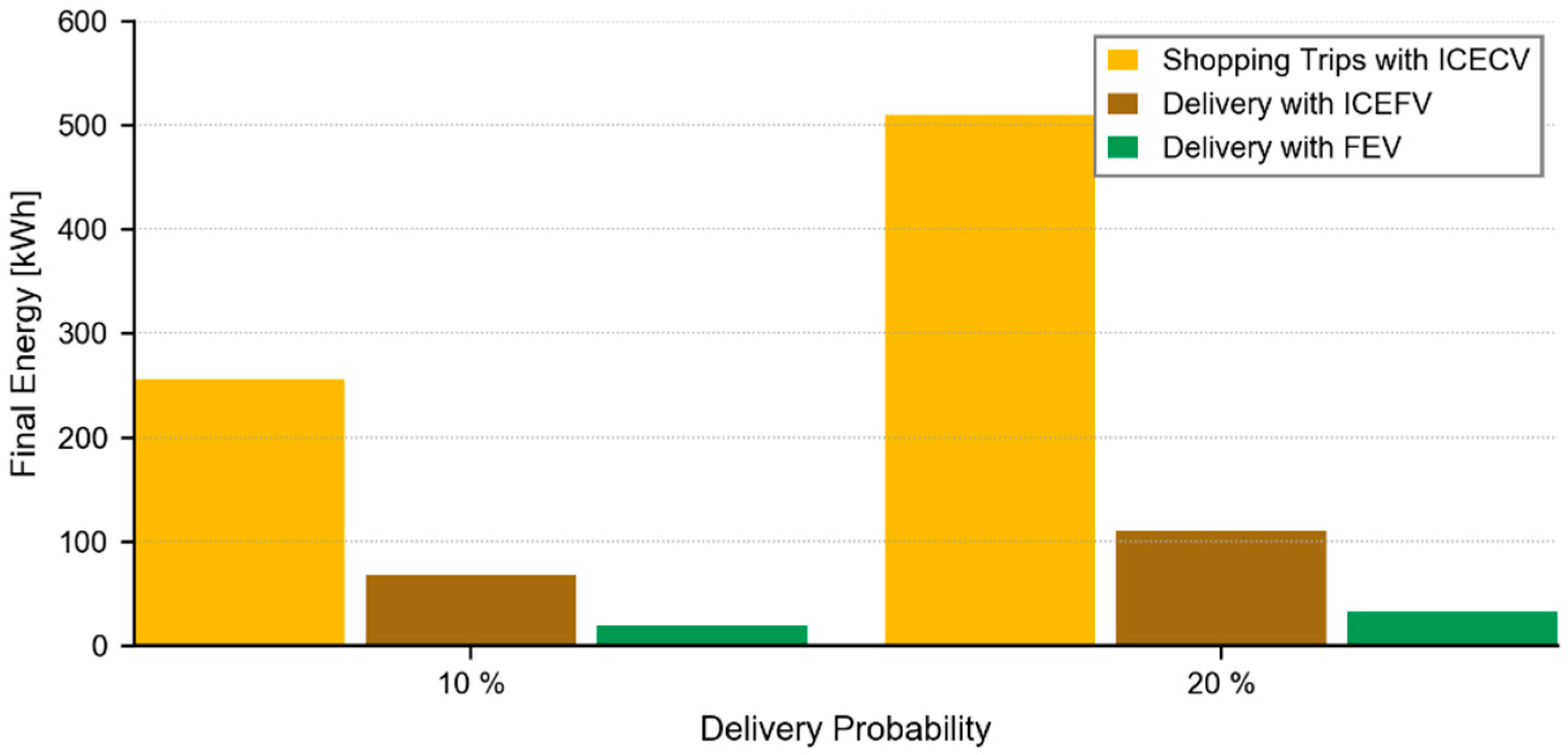
| ICECVs | kWh | 255.7 | 510.1 |
| ICEFVs | kWh | 67.6 | 110.2 |
| Savings (Absolute) | kWh | 188.1 | 399.9 |
| Savings (Relative) | % | 73.6 | 78.4 |
| FEVs | kWh | 19.7 | 32.0 |
| Savings (Absolute) | kWh | 236.0 | 478.1 |
| Savings (Relative) | % | 92.3 | 93.7 |
| Vehicle | Unit | Delivery Probability | |
|---|---|---|---|
| 10% | 20% | ||
| ICECVs | kgCO2 | 67.5 | 134.8 |
| ICEFVs | kgCO2 | 18.0 | 29.4 |
| Savings (Absolute) | kgCO2 | 49.5 | 105.4 |
| Savings (Relative) | % | 73.3 | 78.2 |
| FEVs | kgCO2 | 9.6 | 15.7 |
| Savings (Absolute) | kgCO2 | 57.9 | 119.1 |
| Savings (Relative) | % | 85.8 | 88.4 |
| Delivery Vehicles | Customer Vehicles | Energy Savings | Emission Savings | ||
|---|---|---|---|---|---|
| Delivery Probability | Delivery Probability | ||||
| 10% | 20% | 10% | 20% | ||
| ICEFV | ICECV | 12.3% | 10.0% | 12.4% | 10.1% |
| ECV | 53.9% | 44.1% | 29.4% | 24.0% | |
| FEV | ICECV | 3.6% | 2.9% | 6.6% | 5.4% |
| ECV | 15.7% | 12.8% | 15.7% | 12.8% | |
© 2019 by the authors. Licensee MDPI, Basel, Switzerland. This article is an open access article distributed under the terms and conditions of the Creative Commons Attribution (CC BY) license (http://creativecommons.org/licenses/by/4.0/).
Share and Cite
Hardi, L.; Wagner, U. Grocery Delivery or Customer Pickup—Influences on Energy Consumption and CO2 Emissions in Munich. Sustainability 2019, 11, 641. https://doi.org/10.3390/su11030641
Hardi L, Wagner U. Grocery Delivery or Customer Pickup—Influences on Energy Consumption and CO2 Emissions in Munich. Sustainability. 2019; 11(3):641. https://doi.org/10.3390/su11030641
Chicago/Turabian StyleHardi, Lukas, and Ulrich Wagner. 2019. "Grocery Delivery or Customer Pickup—Influences on Energy Consumption and CO2 Emissions in Munich" Sustainability 11, no. 3: 641. https://doi.org/10.3390/su11030641