The Market Treadmill Against Sustainable Income of European Farmers: How the CAP Has Struggled with Cochrane’s Curse


1
Department of Macroeconomics and Agricultural Economics, Poznań University of Economics and Business, al. Niepodległości 10, 61-875 Poznań, Poland
2
Department of International Economics, University of Zielona Góra, ul. Podgórna 50, 65-246 Zielona Góra, Poland
*
Author to whom correspondence should be addressed.
Sustainability 2019, 11(3), 791; https://doi.org/10.3390/su11030791
Submission received: 24 December 2018
/
Revised: 28 January 2019
/
Accepted: 30 January 2019
/
Published: 2 February 2019
(This article belongs to the Special Issue Sustainability and Social Policy)
Abstract
:Willard Cochrane was the first to introduce the notion that farmers are on a market treadmill, which, in spite of their constant efforts to improve productivity, wears away any profits that might result. Therefore, the essence of the treadmill is that agricultural income does not grow in line with the increase in productivity. Although reasons of this phenomenon are economic in nature, it has caused a serious social problem, i.e., the relative deprivation of farmers’ income. Solving this problem is crucial for ensuring sustainable farming in its social dimension. The aim of the article was, firstly, to answer the question to what extent the concept of the market treadmill in agriculture is still valid for European countries; and secondly, to develop a sectoral model of agricultural income that would test whether the Common Agricultural Policy (CAP) has been successfully struggling with the Cochrane’s treadmill. The authors carried out panel research in a group of 25 countries over the years 1980–2015 in various subperiods. The main conclusion was that the traditionally understood market treadmill has lost significance in Europe, which might be advocated as a long-term value-added aspect of the Common Agricultural Policy (CAP).
1. Introduction
The market treadmill in agriculture is not a new phenomenon. The concept is derived from studies carried out by Willard Cochrane on agriculture in the USA at the end of the 1950s and the beginning of the 1960s [1]. Sometimes, this effect is also called “the drainage of economic surplus” [2]. The essence of the treadmill in agriculture is that farm income does not grow in parallel with increased productivity. To boost agricultural productivity, farmers invest in new technologies and increase the scale of production. However, these efforts do not provide an increase an income, as the demand for food is non-flexible while the prices of agricultural raw materials are flexible. As a result, the marginal revenue from agricultural output decreases, forcing producers to invest in more efficient technologies to maintain profitability. Farmers who are the first to introduce these new technologies (i.e., “early adopters”) derive short-term benefits from lower production costs, thus their income is relatively high. By contrast, farmers who are not able to withstand the pressure of participating in the technological race (i.e., “laggards”) cannot decrease costs and are forced to exit. This is also the explanation why, in the long term, the number of farms steadily decreases. Although reasons of the Cochrane’s treadmill are economic in nature, it has caused a serious social problem, i.e., the relative deprivation of farmers’ income, which was observed in many regions in the world [3,4,5]. Hence, occurrence of “the laggards” increases inequalities among farmers, but also makes the agricultural sector “a laggard” of a national economy. In the EU, the relative deprivation of farmers manifests by the relation of entrepreneurial income in agriculture to a similar income measure in other sectors, which equals on average only 40% [3]. Thus, there is a need for an adequate social policy to prevail against the market treadmill not only by healing its effects but also by breaking the underlying economic mechanism. Many economists argue that after the so-called decoupling reform (see below) the Common Agriculture Policy (CAP) has become more social than economic policy, especially when it comes to the direct payments to farmers. The basic definition of social policy, used inter alia by The Department of Social Policy at the London School of Economics, says: social policy is “an interdisciplinary and applied subject concerned with the analysis of societies’ responses to social need”. This definition fits perfectly to the present CAP priorities: “food quality, environment and countryside” and to a public perception of the CAP: 61% of respondents believe that the CAP benefits all citizens and not just farmers, 62% of respondents (a six point increase since 2015) say that "providing safe, healthy and good quality food" should be the top priority for the EU’s CAP [6]. The market treadmill is a driving force for income inequalities in agriculture and makes an indisputable barrier for the sustainable farming. For this reason we have a strong motivation to check if the present course of the CAP mitigates the treadmill mechanism, which has been relatively neglected in economic and social studies.
In his research, Cochrane stated that it is a myth that agriculture returns to a balance automatically [1]. In what is known as the King effect, periods of increasing supply experience a disproportionately high decrease in prices, which is ultimately disadvantageous for revenue [7,8,9,10]. This effect points to flexible prices as the direct cause of treadmill phenomenon, which can be viewed as a kind of market imperfection since prices ought to act as the explanatory variables according to the neoclassical economics [11]. Similar symptoms were also observed by other economists dealing with natural resource and agricultural economics [12,13]. As the author of the treadmill concept himself said: “the product price treadmill made for an interesting theory, but was never empirically tested” [14]. This is why even today agricultural economists can be divided into those who think that the treadmill has now lost its ‘raison d’être’ because of interventions under agricultural policy, and those who believe that it is a timeless phenomenon. The prices of agricultural raw materials, agricultural incomes and productivity have been studied many times in individual countries [15,16,17]. However, the interdependence of these factors has not been modeled, in particular for the panels of Western and Central-Eastern European countries. Hence, there is no sufficient evidence either for or against the occurrence of “the market treadmill” in contemporary European agriculture. This problem is of a growing importance in the context of Common Agricultural Policy (CAP). This is a quite unique concept over the world, as according to the European Model of Agriculture, farming in Europe should not only be economically competitive, but also contribute to social and environmental standards [18,19]. If European agriculture is in fact still on the market treadmill, meeting long-term sustainability targets is an arduous undertaking since economic efforts do not translate into adequate income growth.
In this paper, we aimed at investigating the occurrence of treadmill phenomenon in European agriculture. The analyses consisted of two steps. First, we analyzed the link between agricultural productivity and incomes using panel data over the years 1980–2015 in various subperiods. We divided countries in two groups as the scale of surplus drainage may depend on a country’s economic development. Richer countries (represented by Old Member States) experienced low price flexibility for food and more flexible supply curves in agriculture. In the presence of a non-flexible demand for food, farmers take less advantage of technological progress. By comparison, in less developed countries (New Member States) with a more flexible demand for food, the advantages primarily go to the farmers [20]. Furthermore, research has shown that price and production fluctuations are stronger in countries with a fragmented agriculture, such as those in Central-Eastern Europe [21]. In the second step, we constructed sectoral panel models to test whether there was any evidence for Cochrane’s treadmill when macroeconomic environment was taken into account. To test this, variables determining agricultural income (price gap, subsidies, interest rates and average wages in national economy as the proxy for economic growth) were included as control variables in line with the Hicks-Hansen model. We tested the hypothesis of whether, due to the common agricultural policy and the growing links between agriculture and macroeconomic environment, the traditionally understood treadmill has lost its significance.
The rest of the paper is organized as follows. In the next section we review how the treadmill evolved, especially in the context of support policy. Then, we describe the data and adopted methodology. The following section presents obtained results with discussion while the last part concludes.
2. The Evolution of Treadmill Concept in the Context of Agricultural Policy
The economic effects of the treadmill have remained similar, however, the notion of the treadmill has been evolving due to the changes of its main drivers [22].
Some researchers [2,23] claimed that usually only first adopters of technological progress in agriculture benefit, because they can decrease cost of production whereas prices do not fall simultaneously. However, this lasts only for a short time and concerns mainly large farms. In the literature, there are also opposite opinions, e.g., Dürr [24], who proved that a smallholder production multiplier is even stronger than that of a large farm; a vast majority of researches agree that the market conditions depreciate small entities. Historically, the main driver of treadmill was flexible prices. If the demand elasticity was calculated as −0.2 in developed countries, then retail prices of agriculture production have to fall by 10% to increase consumption by 2%. However, if a big part of each dollar spent on consumption is absorbed by marketing system, then the price fall should be even greater [23].
Besides the demand-side explanation of the treadmill, the literature offers two additional frameworks: a supply-oriented approach and a behavioral approach. The supply-oriented approach is specifically linked to the agricultural production [25,26] and implies a low mobility of labor and reverse supply curve [27]. Farmers invest in conditions where the expected return on investment is higher than the cost of implementation. Conversely, investment is discouraged if the expected income is lower than the resale value of the purchased assets. However, if the expected revenue is lower than the cost of acquisition but higher than the resale value, capital becomes completely immobile and is “locked” into agriculture. This situation is called the “high-profit trap” [28].
The behavioral approach addresses the problem of maximizing productivity in agriculture, which functions in a different way than in other sectors. The problem lies in the fact that farmers focus on boosting sales rather than increasing marginal productivity. Some studies tried to explain behavioral aspects of farmers’ decisions by limited adaptability to a changing market [29] or by delayed responses to these changes [30].
Research concerning Western European countries has shown that decoupled payments reduce the market’s influence on farmers’ incomes [31]. Nevertheless, subsidies influence agricultural productivity, and thus the treadmill mechanism. The influence of support on the productivity of farms in the EU has already been studied by numerous authors [32,33,34,35], although the results were not conclusive. These studies showed that before the introduction of the decoupling reform, subsidies had a positive influence on production, but a negative impact on productivity After the reform, the conclusions were ambiguous; however, with an emphasis on the fact that the negative impact may occur less often (as regards the impact of subsidies on the total factor productivity—TFP) or not occur at all (as regards the impact on TFP growth dynamics) [34]. If this is so, then decoupling should mitigate the problem of the market treadmill, as it does not stimulate production and capital intensity, but supports income.
Following an agricultural policy consisting of maintaining high prices of agricultural products has led to a shift of the accent to another driving force for the treadmill. Price support improved the profitability of agriculture, and area payments resulted in the capitalization of transfers in agricultural land prices [36,37]. As a result, the demand for agricultural land, and thus its price, increased considerably. Hence, a sui generis fight over a rare resource, i.e., land, began [14]. This placed land owners in a privileged position. They did not have to worry about the treadmill, since the growing prices of the resource they owned made it possible for them to sell land at a good price, or profit from leasing it. In this new situation, not only could the early adopters benefit, but also the farmers in the worst economic situation. They could change the orientation of their activity, and profit from land lease. The ‘average farmers’ were now in the worst situation, as they continued agricultural activity and did not benefit from the increase in land prices, while at the same time were not innovative enough to profit from the implementation of new technologies in agriculture.
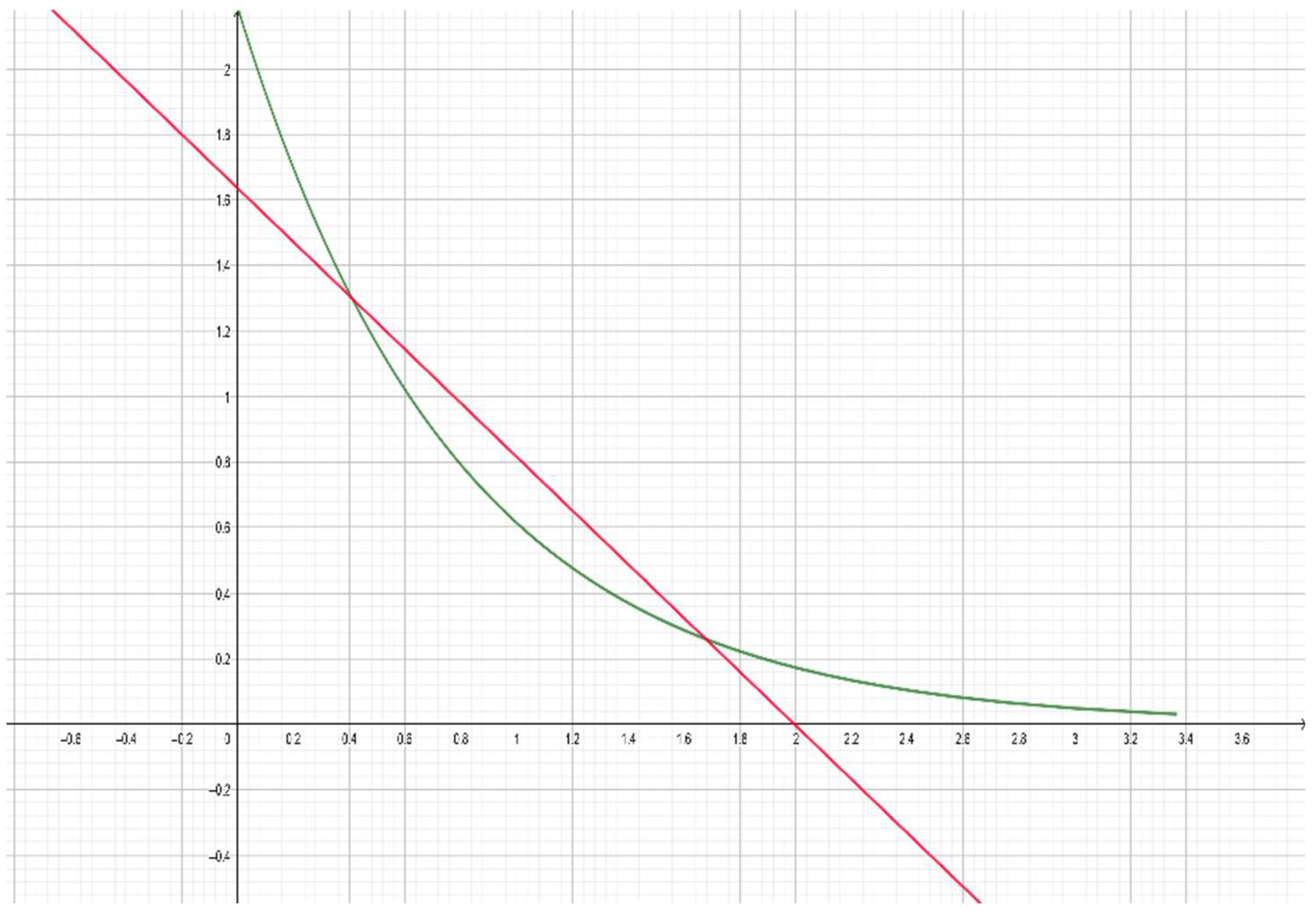
Taking the above evolution under consideration, it is an exponential function that fits best to describe the phenomenon of market treadmill in which the productivity is an explanatory variable for the income (assuming the “−” sign for the productivity coefficient). We present this case in Figure 1, which visualizes the coefficients from Table 2 for the EU15 panel 1980–1994–although it seems paradoxical, the highest income occurs when productivity equals zero. It is the case of a farmer who sells or leases out all his land. It is commonly known that farmers who continue agricultural production would never get a net profit equal to the economic rent discounted in the market value of the land that they own, because the use value of agricultural land explains a diminishing part of a land’s price (this thesis is developed in methodology section). Hence, selling parcels seems to be the best option to capture rents capitalized in land, if short-term economic aspects are taken into account. When farmers increase productivity, the rent gap in relation to the value capitalized in land (entrepreneurial income) is growing, as is shown in Figure 1. However, there is some hypothetical level of productivity where incomes cease to decline while productivity rises (cf. Figure 1). Due to this asymptote that limits the income drop, the exponential model with a negative regression sign reflects properly Cochrane’s idea of the market treadmill and will be engaged in the first step of our analysis.
3. Materials and Methods
3.1. Model Construction
In order to check whether the phenomenon of the treadmill is functioning in European agriculture, we employed a two-steps econometric strategy. In the first step, a phrase in Cochrane’s hypothesis that productivity growth in agriculture does not correspond with a rise of agricultural income has been tested. In the one-variable regression, we used real entrepreneurial income in agriculture, excluding any subsidies for three panels: ‘old’ EU15 Member States (MS) in 1980–1994, ‘old’ EU15 MS in 1995–2015 and ‘new’ EU12 MS in 2004–2015, accessed to the EU in 2004, cf. Table 2. These periods were selected for several reasons: first, a process of reforming CAP (i.e., ‘decoupling’) was initiated in the ‘old’ EU15 by the MacSharry reform in the early 1990 and has been continued by the ‘Agenda 2000’ and ‘Luxembourg CAP reform’ (2003); thus, we assumed its first noticeable effects on farmers income and prices have been occurring since 1995. Second, 2004 is the accession date for the ‘new’ EU12 MS, whose agriculture had operated in a completely different political and institutional framework before this date. Third, we took the 80s as the initial point, because since 1980, there are consistent EUROSTAT data available for a majority of ‘old’ MS. The following specification may address how the ‘pure’ market mechanism reacts to the changes of productivity in the similar conditions of EU membership, to which both panels (UE15 and UE12) were subjected in the analyzed periods. We may assume the “pure market” conditions are realistic, due to the exclusion of the impact of agricultural policy and inflation at the sector level (real prices means that the value of income has been deflated with Harmonised Index of Consumer Prices—HICP). We would reject Cochrane’s hypothesis if a sign of the productivity level (for definition see Table A1.) was positive and significant. Otherwise, we accepted it.
To test the pure relationship between agricultural entrepreneurial income and productivity we used exponential and linear functional forms in panel models:
where: i is the country, t year, and y entrepreneurial income, excluding subsidies at real prices (sector level), relative to agricultural output, (see Table A1) and Space heterogeneity bias and robustness of the models section; u is the random parameter; β is a vector of the dummy variable parameters for the effects of individual countries (dummy units) that control for the space heterogeneity ; λ is a vector of the dummy variable parameters for the period T that control for the time heterogeneity.
lnyit = α0 + α1PRODUCTIVITYit + β’DU + λ’DV + u,
yit = α0 + α1PRODUCTIVITYit + β’DU + λ’DV + u,
We considered a general sense of Cochrane’s theory including his last contribution–the land market treadmill [14]. Hence, it is an exponential function that fits best to the treadmill phenomenon, as it was advocated in the previous section. The statement that farmers, while running agricultural production, would never get a net profit equal to the economic rent discounted in the value of the land, has been advocated by many authors who proved that use value of agricultural land explains a diminishing part of a land’s price [38,39]. There is also another logical explanation for the exponential function: when the share of intermediate consumption in the value of production decreases (ceteris paribus), income grows more than proportionally, due to the growing economies of scale. Moreover, the log-linear model makes it possible for the income to change proportionally with the volume of agricultural production in the given country [40]. However, to compare the explanatory powers of two functional forms, we also ran regressions for basic linear functional forms.
In the second step, we inserted into the model a set of macroeconomic control variables that might theoretically have an influence on the relations of income and productivity and change the sign of the regression in equations 1a and 1b. This set of explanatory variables has been derived on the one hand from the EUROSTAT methodology, and on the other, from the basic relations of disposable incomes, interest rates, and national income growth described in the Hicks-Hansen model [41]. In effect, we added price indices for agricultural output and input (as the price gap index), output subsidies, decoupled subsidies, interest rates and average wages in economy as national income proxy. Price fluctuations and subsidies are those factors excluded in the one-variable version of the model while using “real entrepreneurial income in agriculture without subsidies” as the dependent variable. Thus, if we insert to the model prices and subsidies as the control variables, we have also to change our dependent variable for the “income in current prices”, which encompasses the influence of these two factors according to the EUROSTAT methodology (it would be no sense to test whether prices and subsidies influence the income deprived of the contribution of these factors). Then, we address the macroeconomic impact of interest rates and national income fluctuations as assumed in the Hicks-Hansen model. As a proxy for national income, we used “average wages in the economy” with reference to the modern theory of the relative deprivation of the agricultural incomes [3,4,5,42]. This theory claims that farmers’ income expectations are mostly formulated by the distance to average wages in the economy as a whole reflecting economic growth. The model with control variables is as follows:
where: i is the country, t year, and Y the entrepreneurial income including subsidies at current prices (sector level), relative to agricultural output, see Table A1; β is a vector of the dummy variable parameters for the effects of individual countries that control for the space heterogeneity; λ is a vector of the dummy variable parameters for the period T that control for the time heterogeneity; the definitions of the variables can be found in Table A1.
Yit = α0 + α1PRODUCTIVITYit + α2 PRICE GAPit + α3OUTTPUT SUBSIDIESit + α1DECOUPLED SUBSIDIESit + α1INTEREST RATESi + α1AVERAGES WAGESit + β’DU + λ’DV + u,
Thus, the suggested form of the model actually includes the impact of all the most important macroeconomic aggregates which theoretically influence agricultural income [43], i.e.,: changes in prices, unemployment, interest rates, economic growth rate, currency exchange rate and technological progress, the proxy of which is the technological productivity index. However, the signs of regression coefficients and the relative strength of marginal effects are not entirely clear. We addressed these dilemmas by making estimations of the above-mentioned functions for the panels of the EU15 (1995–2015) and EU12 countries (2004–2015). In the case of the EU12, we used a shorter panel, as these countries have been subjected to support mechanisms since their accession to the EU in 2004. In the models (Table 3), we additionally present standardized regression coefficients to enable their mutual comparisons.
There is also a dilemma concerning the fixed or random effects estimator in the panel regression while testing the market treadmill. We can easily choose the effects using econometric tests. However, the choice between random effects (RE) and fixed effects (FE) should also have theoretical grounds. In the case of Cochrane’s theory, both effects might have a logical explanation: if RE is considered, we can assume that the pricing mechanism is very similar in all countries because agricultural prices are shaped globally. On the other hand, there are some time in-variant country specific market structures or behaviors that justify FE. For this reason, we present both effects in the basic model (Table 2); the right model confirmed by the econometric tests (Breush-Pagan and Hausman) is bolded.
3.2. Space Heterogeneity Bias and Robusteness of the Models
The original version of Cochrane’s theory was built on the basis of macro data observation in the USA [1], thus, we decided to also use a sectoral database to test the market treadmill occurrence in Europe. However, macro data suffers from many problems concerning heterogeneity bias. Nevertheless, we dealt with these in a few ways to minimize the heterogeneity influence. First of all, we expressed the respective variables in the output units (dividing them by the agricultural output in constant prices, without subsidies). Then, fixed effects (FE) or random effects (RE) was used to address respectively time in-variant or space in-variant effects. FE perform this role by attributing time in-variant effects to the country dummies and year dummies, because there are potentially country–specific factors and time-specific factors (e.g., CAP reforms) influencing incomes. RE estimate space in-variant part of the variance, the so-called “between variance”.
There are several potential problems with panel regression that can affect coefficients and inflate standard errors. Usually, panel models encounter three groups of assumption problems: the distribution of residual, groupwise heteroskedasticity and serial correlation, including cross-sectional correlation. Instead of the issue of serial correlation, over the last years, a growing body of literature has been dealing with cross-sectional dependence in panels, which can arise, e.g., if individuals respond to common shocks or if spatial diffusion processes are present, relating individuals in a way depending on a measure of distance [44]. We ran several diagnostic tests for these issues: the Doornik-Hansen test for the distribution of residuals (usually distribution was concentrated but skewness was not a serious issue); a Pesaran test for cross-sectional dependence; and a Wald test that indicated the occurrence of groupwise heteroscedasticity. Usually, we observed these typical problems with the panel data; however, while using Panel Corrected Standard Errors (PCSE), the estimates were quite robust to disturbances of being heteroscedastic and contemporaneously cross-sectionally correlated [45]. The PCSE procedure is recommended for panels with relatively long time series (T) comparing to the number of cross-sections (N), while other procedures, e.g., Heteroskedasticity and Autocorrelation (HAC), are preferable when the time dimension is shorter in relation to N. Due to this fact, our linear and exponential models were estimated using the panel regression method, which engages PCSE robust standard errors or HAC procedure for the sectoral model for EU12. The use of the robust standard errors of Beck-Katz or Arellano (when suitable) can also limit the potential impact of heterogeneity. The selection between the panel and pooled models was made using the Breusch-Pagan test, whereas the Hausman or Welch test was used to determine the choice between the fixed and random effects models. The multicollinearity of the variables was evaluated on the basis of Variance Inflation Factors (VIFs). None of the variables exceed VIF = 2, which is in line with the most radical rules of thumb [46]. It is also not likely that the model encounters endogeneity problems of a revers causality of the income on the productivity or other explanatory variable. We consider the impact of the productivity on the income in the same period, while addressing the autocorrelation as mentioned above. So it is clear that the income derives from the productivity as the relation of an output to an intermediate consumption (costs) in a given year, but not the opposite. The opposite influence might be possible if we insert to the model a lagged productivity, but this is not the case.
3.3. Expected Outcomes
PRODUCTIVITY: the theory of Cochrane’s treadmill argues that a technological progress is a driving force for a farm’s productivity. In the input-output account for agricultural sector the technological progress mainly manifests by the intermediate consumption, which includes operating capital such as: fertilizers and soil improvers, seeds and planting stock, energy, maintenance of materials (machines), maintenance of buildings, agricultural services and other input goods or services. For this reason, we applied a so-called “technical productivity” coefficient, which relates intermediate consumption to the output (both in constant prices). If Cochrane’s treadmill does not work, real entrepreneurial income is a positive function of the technical productivity, understood as the relationship between output and intermediate consumption (i.e., material and services input). Therefore, it is hard to predict the sign for productivity variable in regressions.
PRICE GAP: Income at current prices should be a positive function of the price gap coefficient (defined as the relation of the output price index to the input price index). An increase in output prices faster than an increase in input prices causes the linear growth of income [47].
OUTPUT SUBSIDIES are included in the value of products at current prices according to Economic Accounts for Agriculture (EAA). Income is created by subtracting inputs from this value, and thus, it is a positive linear function of the output subsidies (for definition see Table A1).
DECOUPLED SUBSIDIES are an element of the added value of agriculture according to the EAA. We expect that income is a positive linear function of decoupled subsidies [48,49,50].
INTEREST RATES may influence agricultural income through various channels. Firstly, they constitute an external capital cost and determine the amount of installments. Therefore, in this aspect, income is a negative linear function of an interest rate. Secondly, they constitute a discount rate in the models of land prices (L=R/S, where L is the price of land, R the annual lease fee and S the discount rate [34]. Thus, lower rates mean higher prices of land. This causes an increase in the creditworthiness of farms and drives the land market treadmill described above. Therefore, the influence of interest rate on income may be positive or negative.
AVERAGE WAGES: The direction of the macroeconomic relationship between agricultural income and average wages, being a proxy for the economic growth, is ambiguous. Some studies showed that agriculture is an anti-cyclical area [51], and thus, in better economic circumstances, agricultural income decreases. A better economy means higher wages and lower unemployment. Lower unemployment and an increase in the level of wages in an economy means higher costs of contract work, which is an element of the income in agriculture (this is included in the cost of external production factors). If so, then the relationship between the level of wages in the economy and income should be negative. However, quicker growth means an increase in global demand, including the demand for food (and this translates into higher agricultural income). In the EU12 countries, Engel’s law still works in a limited way, due to the relatively high income elasticity of the demand for food. Therefore, the influence of average wages on income may be positive or negative.
3.4. Descriptive Statistics for Sectoral Models
Throughout the period of 1995–2015, the EU15 countries displayed higher average productivity, although the difference was relatively small (cf. Table 1). Additionally, this gradually became limited, which is indicated by the values for the 2004–2015 subperiods. When it comes to price relationships, the average values of the price gap in the groups of countries under research were at quite a similar level, and their value below 100 indicates that throughout the entire period under study, on average, they took a rather unfavourable course for agriculture. The amount of subsidies weighted by the volume of production was at a higher level in the EU15 countries, although after 2004, the differences have become blurred. Clear differences between the countries were visible in the case of the level of interest rates and remuneration per hour of work. In the so-called new MS, interest rates were at a higher level, while the average hourly wage in the economy was lower (cf. Table 1).
Interestingly, the level of the dependent variables throughout the entire period from 1995 to 2015 was similar in the EU12 and EU15, and after 2004 higher in the EU12. This was influenced by a considerable increase in income with reference to output after 2004. In addition, we needed to remember that, for weighting, we used output at fixed prices and not the number of employees or farms, because the agriculture of the EU12 is characterised by the fragmentation of agricultural structures (large number of farms) and a lower labour productivity connected with over-employment in agriculture. Data on this topic have been presented in many other studies [52,53]. The introduction of these problems to the analysis would make the researched issue of the treadmill unintelligible.
4. Results and Discussion
4.1. Evidence of Treadmill Operation in the Long Term
To begin with, we present changes in technical productivity (defined as in Table A1) in the panel of 15 (EU15) European countries in the years 1980–1994 (cf. Figure 2). The chart shows a significant upward trend. Figure 3 shows the value of real entrepreneurial income in agriculture within the same panel. In the upper section of the chart, the larger countries are concentrated, the smaller ones in the lower. Nevertheless, the downward trend can be observed, at least up to the mid-1990s.
The trends from Figure 2 and Figure 3 should be confirmed through a panel analysis of the regression of real income and technological productivity. As mentioned in the methodology section, agricultural entrepreneurial income was divided by agricultural output at constant prices in order to eliminate heterogeneity in the size of individual economies. Additionally, the value of subsidies was deducted. Taking into consideration the 15 European countries over a period of 15 years, real income was negatively correlated with agricultural productivity and this is a relationship of strong statistical significance in all forms of the applied models (cf. Table 2). We have tested the treadmill theory using the exponential and linear forms. Despite the first one fitting better in theory, the latter turned out to have a two times bigger explanatory power (R2 = 0.12 vs R2 = 0.28, cf. Table 2), thus, we decided to develop the linear model in the sectoral approach.
It is clearly visible that over this period, Cochrane’s treadmill functioned in Europe. Certainly, productivity itself explains the variation of income only to a small degree, hence, in the next section, we estimated the models with the use of multiple control variables. It should be pointed out, however, that if we move the research period to the years 1995–2015 (EU15) and 2004–2015 (for the EU12), the relationship under study changes completely. After 1995, the relationship between productivity and income in European countries is positive (cf. Table 2). Although the 1995 distinction is only a hypothetical date, we can say that since the mid-1990s the market treadmill in its traditional sense has not operated in European agriculture. It is hard to answer precisely why this happened. We may speculate that the CAP evolution with its milestone reforms was a main force that contained Cochrane’s treadmill. The first CAP period before MacSharry’s reform in 1992 boosted production and capital accumulation (especially land concentration) in the agriculture of West-European Countries. As we can see in Figure 2, the productivity rose continuously. In this way the productivity approached a hypothetical level after which incomes cease declining, as it is indicated in the example in Figure 1. Then, CAP implemented a “decoupling” that has been breaking the relationships between subsidies and agricultural output on the one hand, and on the other, has been enhancing agribusiness development by multiple schemes aimed to support the horizontal integration of farmers, shortening marketing channels, providing public goods, etc. These measures do not stimulate agricultural output but also create the value added of agricultural products in different ways, which do not affect the prices flexibility. Thus, the market treadmill did not operate as it did before and a rising productivity, accompanied by economies of scale, easier translates into higher incomes. However, it is worth noting that this evolution would not be possible without the accumulation of capital in agriculture (especially land) that took place in the first period of the CAP’s functioning.
As mentioned above, in the period starting from 1995, a positive relationship of the variables under study can be observed, both among the more developed countries, taking advantage of support mechanisms for a longer period of time (EU15), and in the relatively less developed countries, which have been taking advantage of the CAP after 2004 (EU12). Comparing the regression coefficients in these models, a regularity can be observed that the models for the post-1994 period indicate a weakening of the relationship between productivity and income in absolute values. This may be caused by several factors. Firstly, in connection with the introduction of decoupled payments the stimuli encouraging farmers to increase production decreased as the level of income was raised by direct subsidies. Secondly, capital-intensive intensification may bring increasingly smaller marginal effects.
4.2. Sectoral Model of Agricultural Income in the EU15 and EU12 Countries
As mentioned in the methodology section, apart from the productivity, we introduced the following control variables: price gap, output and decoupled subsidies, long-term interest rates and the average wages in the economy to the model. It is also worth recalling that in the sectoral model, we used agricultural income in current prices with subsidies as a dependent variable.
First, we presented the fixed effects model for the panel of the EU15 countries (Table 3). All the variables included in the model were statistically significant (p-value < 0.01), and the model was well-adjusted (Least Square Dummy Variable—LSDV R2 = 0.90, Within R-Squared = 0.46). Including macroeconomic variables in the model does not change the nature of the relationship between productivity and agricultural entrepreneurial income–it remains positive. As expected, the size of income is positively influenced by subsidies and the improvement of the price gap coefficient (prices of products sold by farmers compared to the prices of products purchased). The interest rate (proxy for the phenomena on the money market) and the averages wages in the economy (illustrating the situation in the labour market) negatively influence the agricultural income. The potential negative impact of the interest rates was explained in the methodology section above. As we can see, the increase in the costs of loans and worsening of the terms of trade in international trade outweigh the positive effects of the increase of creditworthiness and the increase in the prices of agricultural raw materials. Similarly, the negative effects of the increase of wages in the economy (an anti-cyclical issue, the costs of contract work, outflow of workforce from agriculture) were greater than the positive effects of the increase in the demand for food (see the methodology section). As a result, “wages” have a minus sign in the model.
In the context of this paper, the comparison of the marginal power of the impact of the variables under study is of key significance. The coefficient after standardisation in the last columns of Table 3 is used for this comparison. It turns out that the average wages in the economy as a proxy of economic growth is relatively of the largest significance and is followed by the decoupled subsidies. This indicates the considerable dependence of agricultural income on the economic situation in the country and confirms its counter-cyclical behaviour. The interest rate level was also very significant, which yet again indicates the stronger market relationships of the EU15 countries’ agriculture. Productivity in the sector has four times lower significance than wages (ceteris paribus). This shows that efforts to increase productivity can be reflected in agricultural income only to a small degree. It seems that in the EU15 countries, agriculture has entered the next phase of development, in which it is strongly dependent on the external environment and agricultural policy, and to a lesser degree on progress stimulating productivity growth. The interesting thing is that the model indicates that, compared to other factors in the long term, the significance of price relationships for income is relatively small, although it may shape the changes in income in other studies conducted over a shorter period of time, where the level of subsidies and productivity is fairly stable, which show that the significance of this factor grows [54].
In this model, output subsidies did not significantly influence the level of agricultural entrepreneurial income as it was expected after decoupling. What should be noted is the fact that compared to the EU12, the influence of money factors gains significance. This is reflected in the larger significance of interest rates (coefficient −0.011 compared to −0.009 in EU12), the price gap (0.004 compared to 0.001 in EU12) and the lower significance of decoupled subsidies (0.302 compared to 0.661 in EU12)—cf. Table 3. However, the marginal productivity effect is, more than twice as weak (0.056 compared to 0.136).
In the panel of EU12 countries, the fixed effects model was also estimated (cf. Table 3). All of the variables turned out to be statistically significant except for λ (i.e., the vector of dummy variables for years – none of the periods was significant); the years dummies were removed from the model. The directions of influence of the explanatory variables are the same as in the previous EU15 model. The standardised values of the coefficients indicate that it was the long-term interest rates that were of the greatest significance for explaining agricultural income, followed by wages and decoupled payments. When it comes to productivity, the above model indicates that its growth in the relatively less developed countries significantly translated into an increase in agricultural income when including the control variables in the model. However, the question is to what extent this is the effect of low capital intensity, or thanks to SAPS (the Single Area Payment Scheme), which limits production growth to a lesser degree than BPS (the Basic Payment Scheme). We ought to remember that the negative environmental effects connected with increasing productivity in agriculture are less visible in the EU12 and do not limit its growth. In the EU12 countries, larger dynamics of agricultural income growth can generally be observed. This is connected, among others, with a lower income baseline.
5. Conclusions
The first research objective was to ascertain whether the concept of the market treadmill in agriculture is valid for European countries. Taking into consideration a panel of 15 European countries over the 1980–1994 period, real income was negatively correlated with agricultural productivity. This means that, over this period, Cochrane’s treadmill operated in Europe in a similar fashion as it did in the USA, according to Cochrane’s studies.
Moving the research period to the years 1995–2015 (2004–2015 in the case of EU12), the relationship between productivity and income in European countries changed, and was positive. Therefore, we can say that since the mid-1990s, the market treadmill in its traditional sense has not been present in European agriculture.
The disappearance of the treadmill in European agriculture may be linked to the evolution of the common agricultural policy. In its earlier versions (before MacSharry’s reform), policy support was related to the level of production that stimulated the accumulation of capital (mainly land) and the expansion of agricultural holdings. At the same time, growing production, due to the flexible prices, had negative effects on incomes. Decoupling the subsidies from production combined with a support to rural development and the provision of public goods have undermined the effect of the market treadmill since the agricultural value added might be enhanced not only by bigger output but also by higher value added by those means that do not cause such unfavorable changes in flexible prices. Therefore, we can conclude that the agricultural policy, by blurring the treadmill effect, contributes to the growth of sustainability in agriculture. On the one hand, the positive link between productivity and income improves the economic competitiveness of farms. On the other hand, income support contributes to reducing the relative deprivation of farmers.
The second research objective was to develop a sectoral model of agricultural income, which would show the effects of the treadmill compared to other macroeconomic variables determining agricultural income. The following conclusions can be drawn from these sections:
- After the mid-90s, the level of agricultural income was positively influenced by productivity, subsidies and improvement of the price gap (prices of products sold by farmers compared to the prices of products purchased). The interest rates (proxy for the money market) and the average wages in the economy (proxy for national income growth) negatively influenced the agricultural income, which confirmed the counter-cyclical behavior of the agricultural sector.
- In the EU15, compared to the EU12, the impact of money factors was definitely gaining significance. However, the productivity effect was stronger in the latter.
- It was the subsidies, average wages growth in the economy and monetary policy that were of the greatest significance for shaping the agricultural income, more important than productivity. Paradoxically, agricultural prices did not play a great role until after the mid-90s.
Author Contributions
Conceptualization, B.C.; methodology, B.C. and Ł.K.; formal analysis, B.C. and Ł.K.; investigation, B.C., Ł.K. and A.C.; writing—original draft preparation, B.C, Ł.K. and A.C.; writing—review and editing, B.C. and Ł.K.; project administration, B.C.; funding acquisition, B.C.
Funding
This article is founded by the National Science Centre in Poland (Grant No. 2016/21/B/HS4/00653).
Conflicts of Interest
The authors declare no conflict of interest.
Appendix A

Table A1.
Definitions and sources of variables used in the analysis.
| Variable | Description | Source | Expected Sign |
|---|---|---|---|
| Agricultural income in real prices without subsidies (Table 2) | Entrepreneurial income in real prices (2005 = 100) excluding subsidies in million euro. It corresponds to the operating surplus or mixed income deflated with HICP (Harmonised Index of Consumer Prices). It equals: net added value – employee compensation – taxes connected with production – rents and other real estate rental charges to be paid + interest received – interest paid – subsidies on products – other subsidies. | Economic accounts for agriculture – values at real prices [aact_eaa04] | |
| Agricultural income in current prices with subsidies (Table 3) | Entrepreneurial income in current prices including subsidies in million euro. It equals: net added value (including subsidies on products) – employee compensation + balance of other subsidies and taxes connected with production – rents and other real estate rental charges to be paid+ interest received–interest paid | Economic accounts for agriculture – values at current prices [aact_eaa01] | |
| Agricultural output | Production value at producer price (constant prices 2005 = 100) in million euro or in national currencies. Producer price is defined as the price received by the producer without the deduction of taxes or levies (except deductible VAT) and without the inclusion of subsidies. | Economic accounts for agriculture – values at constant prices (2005 = 100) [aact_eaa03] | |
| Productivity level in agriculture (PRODUCTIVITY) | Agricultural output at producer, constant price (i.e., without subsidies) / Total intermediate consumption (materials and services input) at constant, basic price (2005 = 100), both in national currencies. The basic price is the price receivable by the producers from the purchaser for a unit of a good or service produced as output minus any tax payable on that unit as a consequence of its production or sale (i.e., taxes on products), plus any subsidy receivable on that unit as a consequence of its production or sale (i.e., subsidies on products). | Economic accounts for agriculture – values at constant prices (2005 = 100) [aact_eaa03] | +/- |
| Agricultural price gap (PRICE GAP) | Nominal price index, n − 1 = 100 for production value at basic price/Nominal price index, n − 1 = 100 for inputs (i.e., total intermediate consumption at basic price) | Economic accounts for agriculture – indices: volume, price, values [aact_eaa05] | + |
| Output subsidies | Subsidies on products contributing to agricultural output at basic price in Million euro, i.a. price subsidies, animal bonus/Agricultural output | Economic Accounts for Agriculture, Eurostat | + |
| Decoupled subsidies | Other subsidies on production at basic price in million euro includes, inter alia . single area payments and basic (single) payment/agricultural output | Economic accounts for agriculture – values at current prices [aact_eaa01] | + |
| Long-term interest rate (INTEREST RATES) | European Monetary Union EMU convergence criterion bond yields (%), or if EMU not applicable, money market interest rates | EMU convergence criterion series – annual data [irt_lt_mcby_a] Money market interest rates – annual data [irt_st_a] | +/- |
| Average wages in national economy (AVERAGE WAGES) | Gross wages and salaries (excluding social contributions) in million euro / thousand hours worked (employees domestic concept) | GDP and main components [nama_10_gdp] Employment by A*10 industry breakdowns [nama_10_a10_e] | +/- |
Source: Own elaboration on the basis of Economic Accounts for Agriculture, Eurostat.
References
- Cochrane, W.W. Farm Prices: Myth and Reality; University of Minnesota Press: Minneapolis, MN, USA, 1958. [Google Scholar]
- Czyżewski, B.; Majchrzak, A. Market versus agriculture in Poland–macroeconomic relations of incomes, prices and productivity in terms of the sustainable development paradigm. Technol. Econ. Dev. Econ. 2018, 24, 318–334. [Google Scholar] [CrossRef]
- Czyżewski, B.; Poczta-Wajda, A. Effects of Policy and Market on Relative Income Deprivation of Agricultural Labour. In Proceedings of the 160th EAAE Seminar “Rural jobs and the CAP”, Warsaw, Poland, 1–2 December 2016; Available online: http://ageconsearch.umn.edu/bitstream/249759/2/Czyzewski_Poczta-Wajda.pdf (accessed on 12 May 2017).
- Chen, S.; Ravallion, M. More Relatively-Poor People in a Less Absolutely-Poor World. Rev. Income Wealth 2013, 59, 1–28. [Google Scholar] [CrossRef]
- Sen, J.; Prakas Pal, D. Changes in relative deprivation and social well-being. Int. J. Soc. Econ. 2013, 40, 528–536. [Google Scholar] [CrossRef]
- Eurostat. Public Opinion on the Common Agricultural Policy. Available online: https://ec.europa.eu/info/food-farming-fisheries/key-policies/common-agricultural-policy/cap-glance/eurobarometer_en (accessed on 28 January 2019).
- Barret, C.B. On price risk and the inverse farm size-productivity relationship. J. Dev. Econ. 1996, 51, 193–215. [Google Scholar] [CrossRef]
- Evans, G.H., Jr. The law of demand—The roles of Gregory King and Charles Davenant. Q. J. Econ. 1967, 81, 483–492. [Google Scholar] [CrossRef]
- Tweeten, L.; Zulauf, C. Farm price and income policy: lessons from history. Agribus. Int. J. 2008, 24, 145–160. [Google Scholar] [CrossRef]
- Chen, Z.; Huffman, W.E.; Rozelle, S. Inverse relationship between productivity and farm size: The case of China. Contemp. Econ. Policy 2011, 29, 580–592. [Google Scholar] [CrossRef]
- Tomek, W.G.; Robinson, K.L. Agricultural Product Prices; Cornell University Press: Ithaca, NY, USA, 1981. [Google Scholar]
- Barnett, H.J.; Morse, C. Scarcity and Growth: The Economics of Natural Resource Availability; The Johns Hopkins Press: Baltimore, MD, USA, 1963. [Google Scholar]
- Winfrey, W.; Darity, W., Jr. Increasing returns and intensification: A reprise on ester Boserup’s model of agricultural growth. Metroeconomica 1997, 48, 60–80. [Google Scholar] [CrossRef]
- Levins, R.A.; Cochrane, W.W. The treadmill revisited. Land Econ. 1996, 72, 550–553. [Google Scholar] [CrossRef]
- Hayami, Y.; Ruttan, V.W. Agricultural productivity differences among countries. Am. Econ. Rev. 1970, 60, 895–911. [Google Scholar]
- Kijek, T.; Nowak, A.; Kasztelan, A.; Krukowski, A. Agricultural total factor productivity changes in the new and the old European Union members. In Proceedings of the 7th International Scientific Conference Rural Development, Kaunas, Lithuania, 19–20 November 2015. [Google Scholar]
- Restuccia, D.; Yang, D.T.; Zhu, X. Agriculture and aggregate productivity: A quantitative cross-country analysis. J. Monet. Econ. 2008, 55, 234–250. [Google Scholar] [CrossRef]
- Arzeni, A.; Esposti, R.; Sotte, F. Agriculture in Transition Countries and the European Model of Agriculture: Entrepreneurship and Multifunctionality; The World Bank, Šibenik-Knin and Zadar Counties: Framework for a Regional Development Vision; The World Bank: Washington, DC, USA, 2001. [Google Scholar]
- Czyżewski, B.; Matuszczak, A.; Muntean, A. Influence of agricultural policy on the environmental sustainability of European farming. J. Environ. Prot. Ecol. 2018, 19, 426–434. [Google Scholar]
- De Gorter, H.; Swinnen, J. Political economy of agricultural policy. Handb. Agric. Econ. 2002, 2, 1893–1943. [Google Scholar]
- Majchrzak, A.; Stępień, S. Flows of rents as an economic barometer for agriculture: The case of the EU-27. In Political Rents of European Farmers in the Sustainable Development Paradigm. International, National and Regional Perspective; Czyżewski, B. Polish Scientific Publishers PWN: Warsaw, Poland, 2016. [Google Scholar]
- Czyżewski, B.; Matuszczak, A.; Miśkiewicz, R. Public Goods Versus The Farm Price-Cost Squeeze: Shaping The Sustainability of The Eu’s Common Agricultural Policy. Technol. Econ. Dev. Econ. 2019, 25, 82–102. [Google Scholar] [CrossRef]
- Gabre-Madhin, E.; Barrett, C.B.; Dorosh, P. Technological Change and Price Effects in Agriculture: Conceptual and Comparative Perspectives; International Food Policy Research Institute (IFPRI): Washington, DC, USA, 2002. [Google Scholar]
- Dürr, J. The political economy of agriculture for development today: the “small versus large” scale debate revisited. Agric. Econ. 2016, 47, 671–681. [Google Scholar] [CrossRef]
- Heinrichsmayer, W.; Witzke, H.P. Agrarpolitik Band 1: Agrarökonomische Grundlagen; UTB: Stuttgart, Germany, 1991. [Google Scholar]
- Gardner, B.L. Changing economic perspectives on the farm problem. J. Econ. Lit. 1992, 30, 62–101. [Google Scholar]
- Czajanow, A. The Theory of Peasant Economy; The University of Wisconsin Press: New York, NY, USA, 1966. [Google Scholar]
- Johnson, D.G. Reducing the Urban-Rural Income Disparity; University of Chicago: Chicago, IL, USA, 2000; Paper No. 00-07. [Google Scholar]
- Vergopoulos, K. Capitalism and peasant productivity. J. Peasant Stud. 1978, 5, 446–465. [Google Scholar] [CrossRef]
- Boháčková, I. Some notes to income disparity problems of agriculture. Agris On-Line Pap. Econ. Inform. 2014, 5, 2–11. [Google Scholar]
- Cunha, A.; Swinbank, A. An Inside View of the CAP Reform Process: Explaining the MacSharry, Agenda 2000, and Fischler Reforms; Oxford University Press: Oxford, UK, 2011. [Google Scholar]
- Hennessy, D.A. The production effects of agricultural income support policies under uncertainty. Am. J. Agric. Econ. 1998, 80, 46–57. [Google Scholar] [CrossRef]
- Ciaian, P.; Swinnen, J.F. Credit market imperfections and the distribution of policy rents. Am. J. Agric. Econ. 2009, 91, 1124–1139. [Google Scholar] [CrossRef]
- Rizov, M.; Pokrivcak, J.; Ciaian, P. CAP subsidies and productivity of the EU farms. J. Agric. Econ. 2013, 64, 537–557. [Google Scholar] [CrossRef]
- Banga, R. Impact of Green Box Subsidies on Agricultural Productivity, Production and International Trade; Working Paper, Centre for WTO Studies; Indian Institute of Foreign Trade: New Delhi, India, 2014. [Google Scholar]
- Góral, J.; Kulawik, J. Problem of capitalisation of subsidies in agriculture. Probl. World Agric. 2015, 342, 3–23. [Google Scholar] [CrossRef]
- OECD. A Matrix Approach to Evaluating Policy: Preliminary Findings from PEM Pilot Studies of Crop Policy in the EU, the US, Canada and Mexico; OECD Directorate for Food, Agriculture and Fisheries Trade Directorate: Paris, France, 2000. [Google Scholar]
- Czyżewski, B.; Trojanek, R.; Matuszczak, A. The effects of use values, amenities and payments for public goods on farmland prices: Evidence from Poland. Acta Oecon. 2018, 68, 135–158. [Google Scholar] [CrossRef]
- Barnard, C.H. Urbanization affects a large share of farmland. Rural Cond. Trends 2000, 10, 57–63. [Google Scholar]
- Malpezzi, S. Hedonic pricing models: a selective and applied review. Hous. Econ. Public Policy 2002, 67–89. [Google Scholar] [CrossRef]
- Bentolila, S. Hicks-Hansen model. In An Eponymous Dictionary of Economics; Segura, J., Rodríguez-Braun, C., Eds.; Edward Elgar: Cheltenham, UK, 2005. [Google Scholar]
- Fałkowski, J. Does It Matter How Much Land Your Neighbour Owns? The Functioning of Land Markets in Poland from a Social Comparison Perspective; IDEAS Working Paper Series from REPEc; Centre for European Policy Studies: Brussels, Belgium, 2013; pp. 1–20. [Google Scholar]
- Schiff, M.; Valdés, A. Agriculture and the macroeconomy, with emphasis on developing countries. Handb. Agric. Econ. 2002, 2, 1421–1454. [Google Scholar]
- Croissant, Y.; Millo, G. Panel data econometrics in R: The plm package. J. Stat. Softw. 2008, 27, 1–43. [Google Scholar] [CrossRef]
- Hoechle, D. Robust standard errors for panel regressions with cross-sectional dependence. Stata J. 2007, 7, 281. [Google Scholar] [CrossRef]
- Chatterjee, S.; Hadi, A.S. Regression Analysis by Example; John Wiley & Sons: Hoboken, NJ, USA, 2015. [Google Scholar]
- Liefert, W.M. Decomposing changes in agricultural price gaps: An application to Russia. Agric. Econ. 2009, 40, 5–28. [Google Scholar] [CrossRef]
- Hansen, H.; Teuber, R. Assessing the impacts of EU’s common agricultural policy on regional convergence: Sub-national evidence from Germany. Appl. Econ. 2011, 43, 3755–3765. [Google Scholar] [CrossRef]
- Severini, S.; Tantari, A. The effect of the EU farm payments policy and its recent reform on farm income inequality. J. Policy Model. 2013, 35, 212–227. [Google Scholar] [CrossRef]
- Enjolras, G.; Capitanio, F.; Aubert, M.; Adinolfi, F. Direct payments, crop insurance and the volatility of farm income. Some evidence in France and in Italy. New Medit 2014, 13, 31–40. [Google Scholar]
- Da-Rocha, J.M.; Restuccia, D. The role of agriculture in aggregate business cycles. Rev. Econ. Dyn. 2006, 9, 455–482. [Google Scholar] [CrossRef]
- Smit, M.J.; van Leeuwen, E.S.; Florax, R.J.; de Groot, H.L. Rural development funding and agricultural labour productivity: A spatial analysis of the European Union at the NUTS2 level. Ecol. Indic. 2015, 59, 6–18. [Google Scholar] [CrossRef]
- Martín-Retortillo, M.; Pinilla, V. On the causes of economic growth in Europe: Why did agricultural labour productivity not converge between 1950 and 2005? Cliometrica 2015, 9, 359–396. [Google Scholar] [CrossRef]
- Czyżewski, A.; Kryszak, Ł. Agricultural income and prices. The interdependence of selected phenomena in Poland compared to EU-15 member states. Manag. Econ. 2017, 18, 47–62. [Google Scholar] [CrossRef]
Figure 1.
Cochrane’s treadmill in EU15 countries in the years 1980–1994. The red line visualizes the linear function of productivity and income for panel of EU15 countries (1980–1994); the green one visualizes exponential function for the same panel (Table 2); X-axis represents productivity levels, Y-axis represents agricultural income in real prices without subsidies calculated per agricultural output (see Table A1 for definitions). Source: own elaboration based on Eurostat data (Table 2).

Figure 2.
Changes in the value of the productivity coefficient in agriculture for EU15 countries in the years 1980–1994. * productivity coefficient = agricultural output (without subsidies in constant prices)/total intermediate consumption (in constant prices)
Figure 2.
Changes in the value of the productivity coefficient in agriculture for EU15 countries in the years 1980–1994. * productivity coefficient = agricultural output (without subsidies in constant prices)/total intermediate consumption (in constant prices)

Figure 3.
Changes in the value of real entrepreneurial income in agriculture (without subsidies) for EU15 countries in the years 1980–1994. * Real agricultural income without subsidies = net added value − employee compensation − taxes − rents and other real estate rental charges to be paid + balance of interest received and paid − subsidies on products − other subsidies.

Table 1.
Descriptive statistics of variables used to build the sectoral income models for EU15 and EU12.
Table 1.
Descriptive statistics of variables used to build the sectoral income models for EU15 and EU12.
| Variable | EU15 (‘95–‘15) | EU12 (‘95–‘15) | EU15 (‘04–‘15) | EU12 (‘04–‘15) |
|---|---|---|---|---|
| Average wages (euro per hour) | 18.37 | 4.99 | 20.74 | 6.12 |
| (6.74) | (3.28) | (6.86) | (3.15) | |
| Interest rates (%) | 4.67 | 8.85 | 3.76 | 4.84 |
| (2.47) | (2.47) | (3.76) | (2.42) | |
| Entrepreneurial income | 0.28 | 0.30 | 0.27 | 0.35 |
| (0.15) | (0.18) | (0.14) | (0.17) | |
| Productivity | 1.62 | 1.54 | 1.63 | 1.61 |
| (0.41) | (0.31) | (0.40) | (0.32) | |
| Price gap | 98.90 | 98.21 | 99.14 | 98.25 |
| (5.03) | (7.90) | (5.49) | (7.61) | |
| Output subsidies | 0.07 | 0.03 | 0.04 | 0.04 |
| (0.07) | (0.04) | (0.05) | (0.04) | |
| Decoupled subsidies | 0.15 | 0.13 | 0.20 | 0.19 |
| (0.14) | (0.11) | (0.14) | (0.10) |
For detailed definitions of variables see Table A1; standard deviation values in parentheses; source: own calculation based on Eurostat.
Table 2.
Testing Cochrane’s theory: fixed (FE) and random effects (RE) for the regression of the productivity and real entrepreneurial income in agriculture without subsidies for the European countries panels (log-linear and linear models).
Table 2.
Testing Cochrane’s theory: fixed (FE) and random effects (RE) for the regression of the productivity and real entrepreneurial income in agriculture without subsidies for the European countries panels (log-linear and linear models).
| Variable | EU 15 (1980–1994) | EU 15 (1995–2015) | EU 12 (2004–2015) | |||
|---|---|---|---|---|---|---|
| Functional form | Log | Linear | Log | Linear | Log | Linear |
| Number of observations | 161 | 169 | 231 | 340 | 112 | 142 |
| Constant FE | 0.783 | 1.636 *** | −4.462 *** | −0.107 | −3.051 *** | 0.020 |
| (0.710) | (0.203) | (0.334) | (0.087) | (0.539) | (0.047) | |
| Constant RE | −0.342 | 1.327 *** | −4.763 *** | −0.271 *** | −3.719 *** | −0.044 |
| (0.321) | (0.161) | 0.406316 | (0.061) | 0.627007 | (0.067) | |
| Productivity coefficient FE | −1.270 ** | −0.822 *** | 1.234 *** | 0.111 * | 0.625 * | 0.062 * |
| (0.473) | (0.134) | (0.192) | (0.0531) | (0.316) | (0.029) | |
| Productivity coefficient RE | −0.478 ** | −0.591 *** | 1.384 *** | 0.213 *** | 1.001 *** | 0.102 *** |
| (0.188) | (0.090) | (0.229) | (0.039) | (0.365) | (0.037) | |
| Functional form | Log | Linear | Log | Linear | Log | Linear |
| Number of observations | 161 | 169 | 231 | 340 | 112 | 142 |
| Within-R2 in FE models | 0.12 | 0.28 | 0.08 | 0.013 | 0.02 | 0.02 |
| Productivity coefficient mean | 1.48 | 1.606 | 1.612 | |||
| Real income without subsidies mean (€ per output unit) | 0.410 | 0.071 | 0.119 | |||
Illustrative interpretations for linear model: 1995–2015: while increasing productivity coefficient by 0.1 (i.e., 6.2% of the mean coefficient), income increases by 0.011 € per output unit (15,5% of the mean income coefficient); 1973–1994 while increasing productivity coefficient by 0.1 (i.e., 6.8% of the mean coefficient), income decreases by 0.082 € per output unit (20% of the mean income coefficient); Entrepreneurial income is measure in relation to the output (in constant prices, without subsidies) to reduce heterogeneity bias. 1980–1994 covers Belgium 1980-, Denmark 1980-, Germany 1991-, Ireland 1990-, Greece 1993-, Spain 1990-, Italy 1980-, Luxemburg 1985-, Netherlands 1986-, Austria 1990-, Portugal 1980-, Finland 1980-, France 1980-, Sweden 1980-, UK 1980-, according to EUROSTAT availability. EU15 “old” EU MS, EU12 “new” EU MS accessed in 2004. Standard errors in brackets; appropriate model according to the Hausman test in bold
Table 3.
Sectoral panel model explaining changes in agricultural entrepreneurial income related to output in EU15 (1995–2014) and EU12 countries (2004–2015) (fixed effects FE).
Table 3.
Sectoral panel model explaining changes in agricultural entrepreneurial income related to output in EU15 (1995–2014) and EU12 countries (2004–2015) (fixed effects FE).
| Variable | EU15 | EU15 Standardized | EU12 | EU15 Standardized |
|---|---|---|---|---|
| Constans | 0.133 | 0.079 | ||
| (0.093) | (0.093) | |||
| Average wages | −13.612 *** | −0.622 *** | −27.302 * | −0.503 * |
| (2.142) | (0.098) | (13.510) | (0.249) | |
| Interest rates | −0.011 *** | −0.184 *** | −0.009 ** | −0.559 ** |
| (0.002) | (0.034) | (0.003) | (0.188) | |
| Productivity | 0.056 * | 0.153 * | 0.136 *** | 0.240 *** |
| (0.031) | (0.086) | (0.038) | (0.068) | |
| Price gap | 0.004 *** | 0.134 *** | 0.001 * | 0.062 * |
| (0.0007) | (0.023) | (0.001) | (0.033) | |
| Decoupled subsidies related to agricultural output | 0.302 *** | 0.286 *** | 0.661 *** | 0.413 *** |
| (0.083) | (0.079) | (0.196) | (0.006) | |
| Year dummies | Yes | Yes | No | No |
| R2 within | 0.461 | 0.347 | ||
| Least Square Dummy Variable (LSDV) R2 overall | 0.901 | 0.872 | ||
| Akaike Information Criterion (AIC) | −934 | −367 | ||
| Hausman test p value | 0.00 | 0.00 | ||
| Residual standard error | 0.050 | 0.063 |
Standard errors in parentheses; p-values corrected according with Panel Corrected Standard (PCSE) robust procedure for EU15 and Arrellano HAC for EU12. *, **, and *** denote 10%, 5% and 1% significance levels, respectively. Source: own calculations based on Eurostat using Gretl and R software (for variables definition cf. Table A1).
© 2019 by the authors. Licensee MDPI, Basel, Switzerland. This article is an open access article distributed under the terms and conditions of the Creative Commons Attribution (CC BY) license (http://creativecommons.org/licenses/by/4.0/).
Share and Cite
MDPI and ACS Style
Czyżewski, B.; Czyżewski, A.; Kryszak, Ł. The Market Treadmill Against Sustainable Income of European Farmers: How the CAP Has Struggled with Cochrane’s Curse. Sustainability 2019, 11, 791. https://doi.org/10.3390/su11030791
AMA Style
Czyżewski B, Czyżewski A, Kryszak Ł. The Market Treadmill Against Sustainable Income of European Farmers: How the CAP Has Struggled with Cochrane’s Curse. Sustainability. 2019; 11(3):791. https://doi.org/10.3390/su11030791
Chicago/Turabian StyleCzyżewski, Bazyli, Andrzej Czyżewski, and Łukasz Kryszak. 2019. "The Market Treadmill Against Sustainable Income of European Farmers: How the CAP Has Struggled with Cochrane’s Curse" Sustainability 11, no. 3: 791. https://doi.org/10.3390/su11030791
Note that from the first issue of 2016, this journal uses article numbers instead of page numbers. See further details here.